Cyclic exchange neighborhood search technique for the K-means clustering problem

(1)

Cyclic Exchange Neighborhood Search Technique

for the K-means Clustering Problem

by

Nattavude Thirathon

S.B.,

Electrical Engineering and Computer Science

Massachusetts Institute of Technology,

2003

Submitted to

MASSACHUSETTS INSTi OF TECHNOLOGY

JUL 2 0 2004

LIBRARIES

the Department of Electrical Engineering and Computer Science

in partial fulfillment of the requirements for the degree of

Master of Engineering in Electrical Engineering and Computer Science

at the

MASSACHUSETTS INSTITUTE OF TECHNOLOGY

February 2004

o

Massachusetts Institute of Technology 2004. All rights reserved.

A u th or ...

...

Department of Electrical Engineering and Computer Science

January 13 , A004

C ertified by ...

James B. Orlin

Professor of Management Science and Operations Research

Thesis Supervisor

Certified by...

Nitin Pail

-- ProfessQgf

Operations

Research

>The5s Supervisor

Accepted by ...

"Arthur C. Smith

Chairman, Department Committee on Graduate Students

BARK

(2)

(3)

-f--Cyclic Exchange Neighborhood Search Technique for the

K-means Clustering Problem

by

Nattavude Thirathon

Submitted to the Department of Electrical Engineering and Computer Science on January 30, 2004, in partial fulfillment of the

requirements for the degree of

Master of Engineering in Electrical Engineering and Computer Science

Abstract

Cyclic Exchange is an application of the cyclic transfers neighborhood search tech-nique for the k-means clustering problem. Neighbors of a feasible solution are obtained by moving points between clusters in a cycle. This method attempts to improve local minima obtained by the well-known Lloyd's algorithm. Although the results did not establish usefulness of Cyclic Exchange, our experiments reveal some insights on the k-means clustering and Lloyd's algorithm. While Lloyd's algorithm finds the best lo-cal optimum within a thousand iterations for most datasets, it repeatedly finds better local minima after several thousand iterations for some other datasets. For the latter case, Cyclic Exchange also finds better solutions than Lloyd's algorihtm. Although we are unable to identify the features that lead Cyclic Exchange to perform better, our results verify the robustness of Lloyd's algorithm in most datasets.

Thesis Supervisor: James B. Orlin

Title: Professor of Management Science and Operations Research Thesis Supervisor: Nitin Patel

Title: Professor of Operations Research

(4)

(5)

Acknowledgments

This thesis is done with great help from my co-supervisors: Professor Jim Orlin and Professor Nitin Patel. Not only did they teach me technical knowledge, but they also guided me on how to do research and live a graduate student life. My transition from an undergraduate student to a graduate student would not be as smooth without their kindness.

I also would like to thank Ozlem Ergun (now a professor at at Georgia Tech). She introduced me to the Operation Research Center in my second semester at MIT. I worked for her as a undergraduate research assistant on neighborhood search tech-niques for traveling salesman problem and sequential ordering problem. Her research work (under supervision of Professor Orlin) ignited my interests in operations research and resulted in me coming back to do my master thesis at ORC.

Lastly, I am grateful to papa, mama, and sister Ann. Nothing rescues tireness, confusion, and long nights better than a warm family back home.

(6)

(7)

List of Figures

2-1 Data Clustering Examples . . . . 18

2-2 Effects of Units of Measurement on Distance-based Clustering . . . . 19

2-3 Z-score Normalization . . . . 19

2-4 Heirachical Data Clustering . . . . 20

3-1 Undesirable Local Optimum from Lloyd's Algorithm . . . . 27

3-2 Improvement Upon Local Optimum from Lloyd's Algorithm by Cyclic Exchange ... .. ... 28

3-3 Definition of Edges in the Improvement Graph . . . . 29

3-4 Definition of Dummy Nodes in the Improvement Graph . . . . 30

3-5 Subset-disjoint Negative-cost Cycle Detection Algorithm . . . . 31

3-6 An Iteration of Cyclic Exchange Algorithm . . . . 33

3-7 ClusGuass Synthetic Data . . . . 34

3-8 MultiClus Synthetic Data . . . . 34

4-1 Layered Structure of the Software . . . . 38

5-1 Dynamics During Iterations of Lloyd's algorithm and Cyclic Exchanges for Dataset c-100-10-5-5 . . . . 44

5-2 Dynamics During Iterations of Lloyd's algorithm and Cyclic Exchanges for Dataset m-100-10-5 . . . . 45

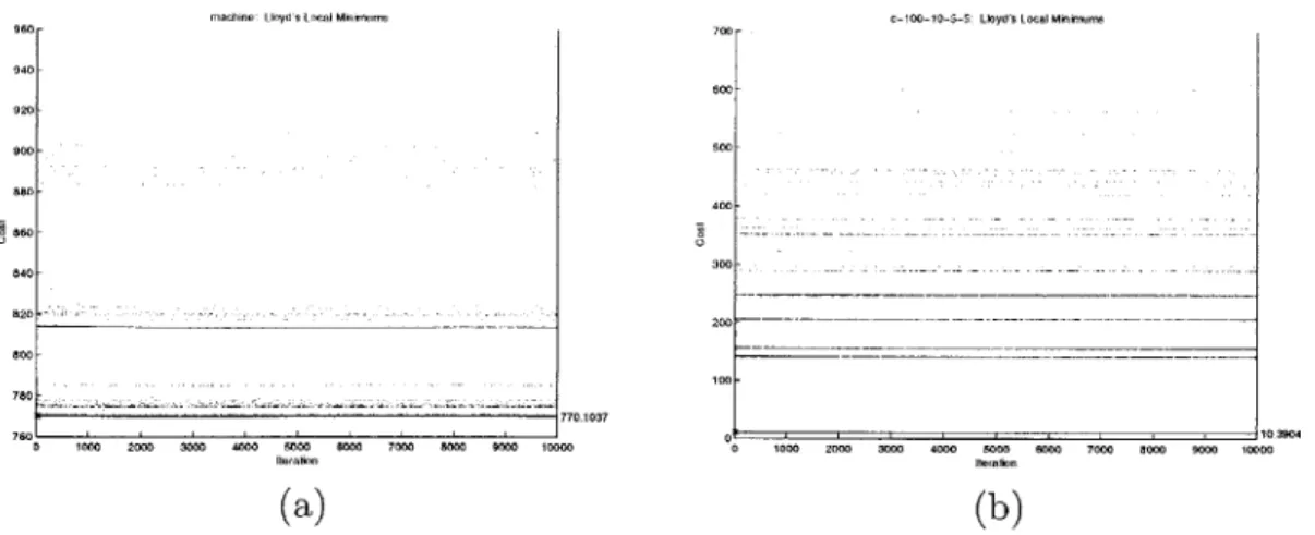
5-3 Costs of Local Minima from Lloyd's Algorithm in 10000 Iterations . . 52

5-4 Structures in the Costs of Local Minima from Lloyd's Algorithm . . . 53

B-1 Layered Structure of the Software . . . . 61 9

(10)

C-1 Iterations C-2 Iterations C-3 Iterations C-4 Iterations C-5 Iterations C-6 Iterations C-7 Iterations C-8 Iterations C-9 Iterations C-10 Iterations C-11 Iterations C-12 Iterations C-13 Iterations C-14 Iterations C-15 Iterations C-16 Iterations C-17 Iterations C-18 Iterations C-19 Iterations C-20 Iterations C-21 Iterations C-22 Iterations C-23 Iterations C-24 Iterations C-25 Iterations C-26 Iterations Lloyd's Lloyd's Lloyd's Lloyd's Lloyd's Lloyd's Lloyd's Lloyd's Lloyd's Lloyd's Lloyd's Lloyd's Lloyd's Lloyd's Lloyd's Lloyd's Lloyd's Lloyd's Lloyd's Lloyd's Lloyd's Lloyd's Lloyd's Lloyd's Lloyd's Lloyd's and and and and and and and and and and and and and and and and and and and and and and and and and and Cyclic Cyclic Cyclic Cyclic Cyclic Cyclic Cyclic Cyclic Cyclic Cyclic Cyclic Cyclic Cyclic Cyclic Cyclic Cyclic Cyclic Cyclic Cyclic Cyclic Cyclic Cyclic Cyclic Cyclic Cyclic Cyclic Exchanges Exchanges Exchanges Exchanges Exchanges Exchanges Exchanges Exchanges Exchanges Exchanges Exchanges Exchanges Exchanges Exchanges Exchanges Exchanges Exchanges Exchanges Exchanges Exchanges Exchanges Exchanges Exchanges Exchanges Exchanges Exchanges for for for for for for for for for for for for for for for for for for for for for for for for for for Dataset Dataset Dataset Dataset Dataset Dataset Dataset Dataset Dataset Dataset Dataset Dataset Dataset Dataset Dataset Dataset Dataset Dataset Dataset Dataset Dataset Dataset Dataset Dataset Dataset Dataset c-100-3-5-5. 98 c-100-5-5-5. 99 c-100-10-5-5 100 c-100-20-5-5 101 c-200-3-5-5. 102 c-200-3-10-5 103 c-200-5-5-5. 104 c-200-5-10-5 105 c-200-10-5-5 106 c-200-10-10-5 107 c-200-20-5-5 108 c-200-20-10-5 109 m-100-3-5 . 110 m-100-5-5 . 111 m-100-10-5 112 m-100-20-5 113 m-200-3-5 . 114 m-200-5-5 . 115 m-200-10-5 116 m-200-20-5 117 covtype-100. 118 glass . . . . . 119 lenses . . . . 120 soybean . . . 121 wine . . . . . 122 zoo . . . . 123

Lloyd's Local Minima for Dataset c-100-10-5-5 . . . .

D-1 D-2 D-3 125 126 126

(11)

D-4 Lloyd's Local Minima for Dataset c-100-5-5-5 D-5 Lloyd's Local Minima for Dataset c-200-10-10-5 D-6 Lloyd's Local Minima for Dataset c-200-10-5-5 D-7 Lloyd's Local Minima for Dataset c-200-20-10-5 D-8 Lloyd's Local Minima for Dataset c-200-20-5-5 D-9 Lloyd's Local Minima for Dataset c-200-3-10-5 D-10 Lloyd's Local Minima for Dataset c-200-3-5-5 D-11 Lloyd's Local Minima for Dataset c-200-5-10-5 D-12 Lloyd's Local Minima for Dataset c-200-5-5-5 D-13 Lloyd's Local Minima for Dataset c-500-10-10-5 D-14 Lloyd's Local Minima for Dataset c-500-10-5-5 D-15 Lloyd's Local Minima for Dataset c-500-20-10-5 D-16 Lloyd's Local Minima for Dataset c-500-20-5-5 D-17 Lloyd's Local Minima for Dataset c-500-3-10-5 D-18 Lloyd's Local Minima for Dataset c-500-3-5-5 D-19 Lloyd's Local Minima for Dataset c-500-5-10-5 D-20 Lloyd's Local Minima for Dataset c-500-5-5-5 D-21 Lloyd's Local Minima for Dataset m-100-10-5 D-22 Lloyd's Local Minima for Dataset m-100-20-5 D-23 Lloyd's Local Minima for Dataset m-100-3-5 D-24 Lloyd's Local Minima for Dataset m-100-5-5 D-25 Lloyd's Local Minima for Dataset m-200-10-5 D-26 Lloyd's Local Minima for Dataset m-200-20-5 D-27 Lloyd's Local Minima for Dataset m-200-3-5 D-28 Lloyd's Local Minima for Dataset m-200-5-5 D-29 Lloyd's Local Minima for Dataset m-500-10-5 D-30 Lloyd's Local Minima for Dataset m-500-20-5 D-31 Lloyd's Local Minima for Dataset m-500-3-5 D-32 Lloyd's Local Minima for Dataset m-500-5-5 D-33 Lloyd's Local Minima for Dataset covtype-100

. . . . 127 . . . . 127 . . . . 128 . . . . 128 . . . . 129 . . . . 129 . . . . 130 . . . . 130 . . . . 131 . . . . 131 . . . 132 . . . 132 . . . 133 . . . 133 . . . 134 . . . 134 . . . 135 . . . 135 . . . 136 . . . . 136 . . . . 137 . . . . 137 . . . . 138 . . . . 138 . . . . 139 . . . . 139 . . . . 140 . . . . 140 . . . . 141 141 11

(12)

D-34 Lloyd's Local Minima for Dataset covtype-200 . . . . 142

D-38 Lloyd's Local Minima for Dataset diabetes . . . . 144

D-39 Lloyd's Local Minima for Dataset glass . . . . 144

D-40 Lloyd's Local Minima for Dataset housing . . . . 145

D-41 Lloyd's Local Minima for Dataset ionosphere . . . . 145

D-42 Lloyd's Local Minima for Dataset lena32-22 . . . . 146

D-43 Lloyd's Local Minima for Dataset lena32-44 . . . . 146

D-44 Lloyd's Local Minima for Dataset lenses . . . . 147

D-45 Lloyd's Local Minima for Dataset machine . . . . 147

D-46 Lloyd's Local Minima for Dataset soybean . . . . 148

D-47 Lloyd's Local Minima for Dataset wine . . . . 148

(13)

List of Tables

3.1 List of Applications Data. . . . . 35

5.1 Comparison between Lloyd's algorithm and Three Versions of Cyclic

Exchanges ... ... 43

5.2 Results for Continue Cyclic Exchange with Two-point Preclustering . 49

5.3 Results for Continue Cyclic Exchange with Birch Preclustering . . . . 51

5.4 The Cost Decreases for Lloyd's Algorithm in 10000 Iterations . . . . . 54

5.5 Results for Two-stage Algorithm . . . . 56

(14)

(15)

Chapter 1 Introduction

Clustering is a technique for classifying patterns in data. The data are grouped into clusters such that some criteria are optimized. Clustering is applicable in many domains such as data mining, knowledge discovery, vector quantization, data com-pression, pattern recognition, and pattern classification. Each application domain has different kinds of data, cluster definitions, and optimization criteria. Optimization criteria are designed such that the optimal clustering is meaningful for the applica-tions.

Clustering is a combinatorially difficult problem. Although researchers have de-vised many algorithms, there is still no known method that deterministically finds an exact optimal solution in polynomial time for most formulations. Thus, the clustering

problems are usually approached by heuristics - relatively fast methods that find

near-optimal solutions.

[7]

gives an overview of many clustering techniques, most of

which are heuristics that find suboptimal but good solutions in limited time. This thesis explores a heuristic for solving a specific class of clustering problem

-the k-means clustering. In -the k-means clustering, data are represented by n points

in d-dimensional space. Given a positive integer k for the number of clusters, the problem is to find a set of k centers such that the sum of squared distances from each point to the nearest center is minimized. Equivalently, the sum of squared distances from cluster centers can be viewed as total scaled variance of each cluster.

A conventional and very popular algorithm for solving the k-means clustering is 15

(16)

Lloyd's algorithm, which is usually referred to as the k-means algorithm. Lloyd's algorithm has an advantage in its simplicity. It uses a property of any locally opti-mal solution that each data point has to belong to the cluster whose center is the nearest. Beginning with a random solution, Lloyd's algorithm converges quickly to a local optimum. Nonetheless, the k-means clustering has tremendous number of local optima, and Lloyd's algorithm can converge to bad ones, depending on the starting point. Our algorithm tries to overcome this limitation of Lloyd's algorithm.

The technique that we propose is an application of a wide class of optimization heuristic known as neighborhood search or local search. Neighborhood search tech-niques try to improve the quality of solution by searching the neighborhood of the current solution. The neigborhood is generally a set of feasible solutions that can be obtained by changing small parts of the current solution. The algorithm searches the neighborhood for a better solution and uses it as a new current solution. These two steps are repeated until the neighborhood does not contain any better solutions. The definition of neighborhood and the search technique are important factors that affect the quality of final solution and time used by the neighborhood search.

This thesis is a detailed report of our work in developing the Cyclic Exchange algorithm. We first give a background on the k-means clustering and neighborhood search, upon which Cyclic Exchange is developed. The detailed descriptions of the algorithm and software development are then presented. This software is used as a back-end for our experiments in the subsequent chapter. We conducted three ex-perimental studies in order to improve the performance of Cyclic Exchange. Each experiment reveals insights on the k-means clustering and Lloyd's algorithm.

(17)

Chapter 2 Background

2.1 Data Clustering

The problems of data clustering arise in many contexts in which a collection of data need to be divided into several groups or clusters. Generally, the data in the same clusters are more similar to one another than to the data in different clusters. The process of clustering may either reveal underlying structures of the data or confirm the hypothesized model of the data. Two examples of data clustering are shown in Figure 2-1. In Figure 2-1(a), the data are represented by points in two dimensional space, and each cluster consists of points that are close together. Figure 2-1(b) from [7] shows an application of data clustering in image segmentation.

Another field of data analysis, discrimination analysis, is similar to but

fundamen-tally different from data clustering. [7] categorizes data clustering as unsupervised

classification, and discrimination analysis as supervised classification. In unsupervised classification, unlabeled data are grouped into some meaningful clusters. In contrast, in supervised classification, a collection of previously clustered data is given, and the problem is to determine which cluster a new data should belong to.

There are generally three tasks in data clustering problems. First, raw data from measurements or observations are to be represented in a convenient way. We then have to define the similarity between data, i.e. the definition of clusters. Lastly, a suitable clustering algorithm is applied. All three tasks are interrelated and need to

(18)

I IA

A I

(a) (b)

Figure 2-1: Data Clustering Examples: (a) Distance-based clustering. (b) Clustering

in image segmentation application [7] - original image and segmented image.

be carefully designed in order to efficiently obtain useful information from clustering. Data can be categorized roughly in to two types: quantitative and qualitative. Quantitative data usually come from physical measurements, e.g. positions, bright-ness, and number of elements. They can be discrete values (integers) or continuous values (real numbers). The use of computer to solve clustering problems, however, re-stricts the continuous-value data to only rational numbers, which can be represented by finite digits in computer memory. Since measurements usually involve more than a single number at a time, e.g. a position in three dimensional space consists of three numbers, quantitative data are usually represented by vectors or points in multidi-mensional space.

Qualitative data come from abstract concepts (e.g. colors and styles), from qual-itative description of otherwise measureable concepts (e.g. good/bad, high/low, and bright/dim), or from classification (e.g. meat/vegetable/fruits). [5] proposed a gener-alized method of representing quantitative data. Qualitative data clustering is beyond the scope of the k-means clustering and is mentioned here only for completeness.

The notion of similarity is central to data clustering as it defines which data should fall into the same cluster. In the case of quantitative data which are represented by points in multidimensional space, similarity is usually defined as the distance between two data points. The most popular distance measure is the Euclidean distance, which can be interpreted is proximity between points, in a usual sense. Other kinds of

(19)

(a) (b)

Figure 2-2: Effects of Units of Measurement on Distance-based Clustering: The hor-izontal unit in (b) is half of those in (a), and the vertical unit in (b) is eight times of those in (a).

Figure 2-3: Z-score Normalization

distance measures include Manhattan distance and higher order norm, for example. The use of distance as similarity function is subject to scaling in units of measure-ments. Figure 2-2 shows two sets of the same data measured in different units. For instance, the horizontal axis represents positions in one dimension, and the vertical axis represents brightness. If the data are grouped into two clusters, and the similar-ity is measured by the Euclidean distance, the optimal solutions are clearly different as shown.

Z-score normalization is a popular technique to overcome this scaling effect. The data is normalized separately for each dimension such that the mean equals to zero and the standard deviation equals to one. Both measurements in Figure 2-2 are normalized to the data in Figure 2-3. If normalization is done every time, the resulting clustering will be the same under all linear units of measurement.

19

(20)

Composition of milk of 25 mammnials Hippo Ho re Monkey O-am itan-Donkey Mule Zebra-Camel Llama-Bison Elephant Buffalo Sheep Fox Pig Cat Dog Rat Deer Reineer Whale Rabbit Dolphin Seal

Figure 2-4: Heirachical Data Clustering [4]

Given the representation of data and the definition of similarity, the remaining task is to find or develop a suitable algorithm. Each algorithm differs in several

aspects. [7] gives a taxonomy of data clustering algorithms. Some of the different

aspects of algorithms are:

" Heirachical v.s. Partitional: A partitional approach is designed to cluster data

into a given number of cluster, such as those in Figure 2-1. In contrast, heirachi-cal approach produces a nested structure of clusters. Figure 2-4 shows an

exam-ple of results for heirachical clustering of a samexam-ple dataset in [4]. By examining

this nested structure at different level, we can obtain different number of clus-ters. Determining the number of clusters for partitional algorithms is a research problem in its own and much depends on the application domains.

" Hard v.s. Fuzzy: A hard clustering assigns each data point to one and only

(21)

membership to several clusters.

" Deterministic v.s. Stochastic: A deterministic approach proceeds in a preditable manner, giving the same result everytime the program is run. A stochastic approach incorporates randomness into searching for the best solution. It may terminate differently each time the program is run.

* Incremental v.s. Non-incremental: An incremental approach gears toward large scale data clustering or online data clustering, where all data are not available at the same time. A non-incremental approach assumes that all of the data are readily available.

As we will see later, Cyclic Exchange algorithm and Lloyd's algorithm are parti-tional, hard, stochastic, and non-incremental.

2.2 K-means Clustering

2.2.1 Notations and Problem Definition

The input of k-means clustering problem is a set of n points in d-dimensional real space and a positive integer k, 2 < k < n. The objective is to cluster these n points into k exhaustive and disjoint sets (i.e. hard clustering), such that the total sum of the squared distances from each point to its cluster center is minimized.

Denote the input points set by X = {x1,. . . , x}, x E !Rd, Vi: 1 <i K n Let each cluster be described by a set of index of the points that belong to this cluster, namely

Cj={i I xi belongs to cluster

j},

Vj : 1

j

< k

Let n be the cardinality of Cj, then the center or the mean of each cluster is 1

mi = - E xi

ni iEC,

(22)

Note that the condition that all clusters are disjoint and exhaust all the input data points means

CjinC

2 =0

,

Vjij 2 :1 ji<j 2 k

and CU ... UCk{1=,...,nJ

Using the notations above, the total sum of the squared distances from each point to its cluster center is

k

V) = E E lxi - mj l2 (2.1)

i=1 iECj

where 11 denotes a Euclidean norm. This cost function can also be interpreted as

the sum of scaled variances in each cluster since 1 siECj flxi - mj112 is the variance of all points in cluster j. These clusters variances are then scaled by cluster sizes nj and added together.

Our problem is then to find m1, ... , Mk, or equivalently Cl,... , Ck, to minimize

V) in Eq. 2.1. Since moving a point from one cluster to another affects two clusters,

namely CjI and C2

,

mjl and mi2 must be recomputed. The inner sum EiC3 lHxi

-m ll2 -must also be reco-mputed for the two clusters. Thus, the definition of the cost in Eq. 2.1 is rather inconvenient for the description and the implementation of algorithms that often move data points around. We instead derive a more convenient cost function as follow.

Let R be the mean of all data points, namely R = 1 xi, and let w be the total

sum of squared distance from R, i.e.,

n i2222 T lixi - R||2 k =E E |xi - Ril2 j=1 iCCj k = 22 |(xi - mj) + (mj - )112 j=1 iE Cj

(23)

((xi - mj)'(xi - m) + 2(xi - mj)'(mj - x) + (m - x)'(mj - x)) lixi- Mj 2 +2 k EE (m3 -x)'(xi j=1 iCCl k j=1 iECi k j=1 iECj k j=1 iCj k j=1 iEC -n3 mj - x112

Y

iECj k = )+Enjlmj _- _R|1 j=1

where the last equality follows from the definition of b in Eq. 2.1 and the fact that the sum of the difference from the cluster mean to all points in the cluster is zero. The second term in the last equality can be further simplified as follow.

=En1mmj -j=1 k =E n m mj j=1 k -nj j=1 k j= n j=1 mj'ri

(

1j k1 j=1 1j k k 2 5 njmj R + nj 'i j=1 j=1 k - 2 1 njmj R + nR'R (=1 - n IIRI12 1: xi -n IRI12 iECj E xi/ iECj 2 xi - n|II12 iECj

Substitute this term back, we get

k T =0+1 j=1 1-2 5 xi - n|lR112 iECj =- n| |CC _h+ j=1

Ni

-iE 23 k flx - mj12 +2E(mj - R)' j=1 k 5 nj||mj j=1 - 1|2 k E j=1 nj

(24)

Since T and nIxRI1 2 are constant, minimizing V) is equivalent to maximizing

#

where

2 _(2.2)

j=1 nI i-Ci

This equivalent cost function is convenient since we can maintain the linear sums of all points in each cluster. Moving a point between two clusters requires updating only two linear sums, their norms, and a few elementary operations. The description

of the cyclic exchange algorithm will be upon solving the problem of maximizing

#

as defined in Eq. 2.2.

2.2.2 Existing Works

Lloyd's Algorithm

Lloyd's algorithm was originated in the field of communication. [11] presented a method for finding a least squares quantization in pulse code modulation (a method for representing data as signals in a communication channel). The data of this prob-lem is the probability distribution of the signal, rather than discrete data points. However, the methods are generalized to work with data points in multidimensional space.

[11] notes that any local minima of quantization problem must satisfy two condi-tions:

" A representative value must be the center of mass of the probability distribution in the region it represents, i.e. the representative values are the conditional expected values in the respective regions.

" A region boundary must be the mid-point of two adjacent representative values. These two conditions can be stated, respectively, in data clustering context as: " Each cluster center must be the center of mass of the data in that cluster. " Each data point must belong to the cluster with the nearest center.

(25)

Based on these two conditions, Lloyd's algorithm starts with a random initial cluster centers. Then, it assigns each data point to the nearest cluster and recomputes the center of mass of each cluster. These two steps are repeated until no data point can be moved. Hence, the two conditions above are satisfied, and we reach a local minimum.

However, these two conditions are only neccessary but not sufficient for the global minimum. The local minimum that Lloyd's algorithm obtains depend much on the initial solutions [12].

Variants of Lloyd's Algorithm

[10] proposed a deterministic method for running multiple (nk) iterations of Lloyd's algorithm to obtain the claimed global optimum. The method incrementally finds

optimal solutions for 1, ... , k clusters. It relies on the assumption that an optimal

solution for k clustering can be obtained via local search from an optimal solution

for k - 1 clustering with an additional center point to be determined. Although [10]

claims that this method is "experimentally optimal", it does not give a rigorous proof of its underlying assumption.

[8] and [10] use k-dimensional tree to speed up each iteration of Lloyd's algorithm. K-dimensional tree is a generalized version of one-dimensional binary search tree. It expedites searching over k-dimensional space and can help Lloyd's algorithm find the

closest center to a given point in time O(log n), as opposed to O(n) by a linear search.

[9] combines Lloyd's algorithm with a local search algorithm, resulting in better solutions. The local search algorithm is based on swapping current cluster centers with candidate centers, which are in fact data points. The algorithm is theoretically proven to give a solution within about nine times worse than the optimal solution, and empirical studies show that the algorithm performs competitively in practice.

(26)

2.3 Neighborhood Search Techniques

Many combinatorial optimization problems are computationally hard. Exact algo-rithms that deterministically find optimal solutions usually take too much time to be practical. Therefore, these problems are mostly approached by heuristics. Neigh-borhood search is a class of heuristics that seek to incrementally improve a feasible

solution. It is applicable to many optimization problem.

[1]

gives an overview of the

neighborhood search.

Neighborhood search begins with an initial feasible solution, which may be ob-tained by randomizing or by another fast heuristic. Then, the algorithm searches the

neighborhood - a set of feasible solutions obtained by deviating the initial solution. The solutions in neighborhood include both better and worse solutions. As a rule of thumb, the larger the neighborhood, the more likely it contains better solutions, but at the expense of a longer search time. The algorithm then searches the neighborhood for a better solution, uses it as a current solution for generating neighborhood. When there is no better solutions in the neighborhood, the current solution is callled locally optimal, and the algorithm terminates.

(27)

Chapter 3 Cyclic Exchange Algorithm

3.1 Motivation

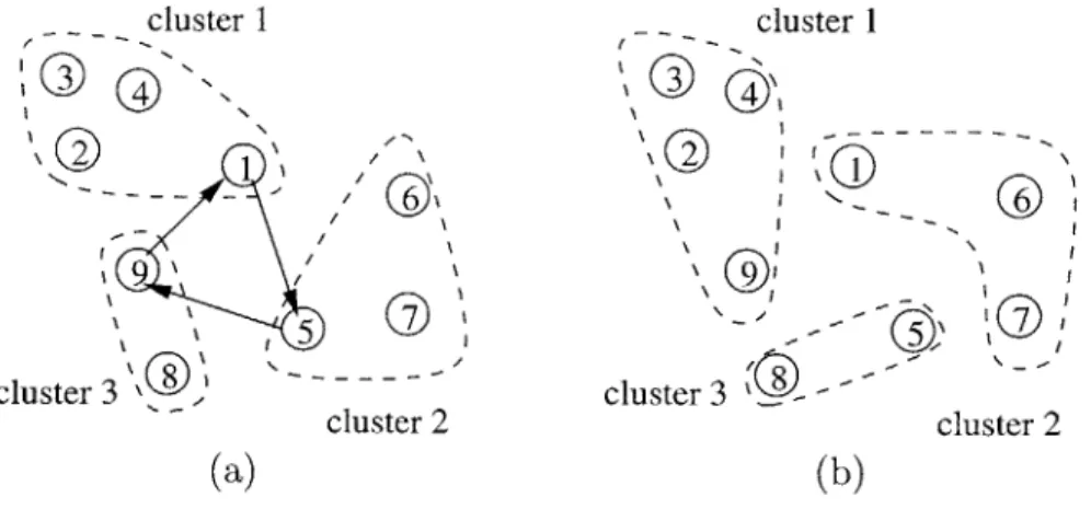
The popular Lloyd's algorithm converges quickly to local optima. At each step, Lloyd's algorithm moves only one data point to a different cluster and thus limits the search space. Sometimes the local optimum can be improved by moving multiple points at the same time. Consider data in Figure 3-1. Lloyd's algorithm converges to the solution portrayed in the figure. There is no way to move a single point and further

improve this solution. Then, consider a moving technique depicted in Figure 3-2. In this case, the solution is of better quality than the previous Lloyd's local optimum. This method moves multiple points at once (the intermediate solutions are of worse quality than the original one). As will be seen, we model this movement as a cycle in an improvement graph, hence the name Cyclic Exchange algorithm. The use of

cyclic transfers in combinatorial optimization problem was pioneered by

[13].

One technique to improve the solution quality of Lloyd's algorithm is to run the

cluster 1 _{cluster 2}

cluster 3

Figure 3-1: Undesirable Local Optimum from Lloyd's Algorithm 27

(28)

clusteri cluster2 cluster 3 cluster 2 cluster I cluster 3 cluster 1 - - - cluster 2 cluster 3 Q

Figure 3-2: Improvement Upon Local Optimum from Lloyd's Algorithm by Cyclic Exchange: Node 2 is moved to cluster 2. Node 3 is moved to cluster 3.

algorithm multiple times using different initial solutions and choose the best local optimum solution as the final answer. This stil leaves room for improvement in many cases. Potentially better solutions may be found in the set of local optimums from

Cyclic Exchange.

3.2 Descriptions of the Algorithm

In neighborhood search, we must first define the neighborhood of any feasible solution. Then, we have to find an efficient way to search the neighborhood for a better solution. In the case of Cyclic Exchange, we define a neighborhood of a solution as a set of solutions that can be obtained by moving multiple data points in a cycle. This movement is described by a cycle in an improvement graph, which we now define.

Let the current feasible solution be (C1,..., Ck). We define a weighted directed graph

g

= (V, 8). V ={1, ... , ,}U{d 1,..., dk}, where the set {1, .. . , n} are nodes

for each data point, and the second set are dummy nodes for each cluster. For

each pair of non-dummy nodes i1 and i2, there is an edge (i1 , i2) if and only if the corresponding data points are in different clusters. In other words, (i1, i2) E E

(29)

cluster I cluster 3 cutr a cluster 2 (a) cluster 1 G) cluster 3 cl (b)

Figure 3-3: Definition of Edges in the Improvement Graph: (a) Current solution and a cycle (1, 5, 9). (b) Resulting solution after applying the cycle.

An edge (i1, i2) represents moving xi, from cluster

Ji

to cluster '2 and moving ₂

out of cluster

j2.

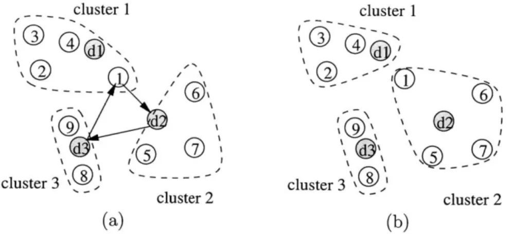
Figure 3-3 shows the effect of cycle (1, 5, 9, 1) if it is applied. The edge (1, 5) substitutes node 1 for node 5 in cluster 2. Node 5 is then left afloat (not in any particular cluster). The edge (5, 9) then puts node 5 in cluster 3, again leaving node 9 afloat. The edge (9, 1) puts node 9 in cluster 1, and hence closes the cycle.

The weight of the cycle must relate the currect cost of the solution to the new cost. We let the change in cost (in term of

#

in Eq. 2.2) be the negative of the weight of the cycle. Let the weight of (i1, i2) be the cost of substituting node Zi for node

i2 in the cluster where i2 is currently in, i.e., C2 , and leave i2 afloat. Note that this

edge affects only the cluster Ch2, and does not affect C31. We find the weight w(i1, i2

)

as follow.

(i1, i2) -

#current

-

#new

(only the term for cluster Cj2 is affected)

2 /2

= _n1 Zx ( xi -xi ₂+xil

3 'Cic

nj

'cj ₂

With this definition of the improvement graph, however, we are constrained to move exactly k nodes in a cycle. This restriction is undesirable as any neighbor has cluster of the same size. Also, we want Cyclic Exchange to be more general than

29

(30)

cluster 1 cluster 1 d d cluster 3 ~) cluster 3 \\G cluster 2 c ~ cluster 2 (a) _(b)

Figure 3-4: Definition of Dummy Nodes in the Improvement Graph: (a) Current

solution and a cycle (1, d2, d3, 1). (b) Resulting solution after applying the cycle.

Lloyd's algorithm. Moving only one data point at at time should also be permitted. Therefore, we introduce dummy nodes dl, . . . , dk, which do not represent data points but represent clusters. More precisely, an edge (i, dj) represents moving of node i to cluster

j

_{and ejecting no points from cluster}_j. _{Similarly, an edge (dj, i) represents} moving no points to the cluster where i is currently in, but instead ejecting i from that cluster. An edge (dj₁, dj2_{) represents no movement but is present to allow no}

movement in some clusters. Figure 3-4 shows the effect of a cycle (1, d2, d3, 1), which

simply moves node 1 to cluster 2.

The costs of edges to and from a dummy node are:

w(i, dj) =- 2 xi + xi 2 2 nj iECj Thj + 1 iECj w(dj,i) = 1 x 1 ( x) - xi nj iEC₃2 fl - 1 _iEC 2

(let i be currently in cluster j2)

w(djl, d2) = 0 (no movement)

With this definition of nodes and edges, the number of nodes in the improvement graph is IVI = _{n + k, and the number of edges is}

VE1

₌_{O((n + k)}2_{). Now, we have}

(31)

procedure Negative-cost Cycle Detection:

input: improvement graph

g

= _{(V, E), number of cluster k}

output: a negative-cost cycle W* begin Pi+-{(i,)E w(ij) < 0} W* -0 while / < k and w(W*) > 0 do begin while Pk -# 0 do begin

remove a path P from P,

let i <-- _{head[P] and h}_<-_tail[P]

if (i, h) EE and w(P) + w(i, h) < w(W*) then W* PU {(i, h)}

for each (i,j) E 8(i) do

begin

if label(j) V LABEL(P) and w(P) + w(i, j) < 0 then

begin

add the path P U{(ij)} to Pk+I

if Pk+1 contains another path with the same key as P

U{(i,

_h)}

then remove the dominated path end end end k <-e k + end end

Figure 3-5: Subset-disjoint Negative-cost Cycle Detection Algorithm (reproduction of Fig.2 in [2])

(32)

new solution is equal to the current cost minus the cost of the improvement cycle, we search for a cycle in the improvement graph with a negative cost.

Instead of enumerating the improvement graph explicitly and searching for a negative-cost cycle, we take an advantage of a special structure of the improvement graph and generate only portions of the improvement graph in which we are actively searching. There are no edges between nodes within the same clusters, and all clus-ters are disjoint. Therefore, we are looking for a negative-cost cycle with all nodes in different clusters, in a graph with n + k nodes. We employ a subset-disjoint negative-cost cycle detection algorithm from [2] and is shown in Figure 3-5. The subsets in

the algorithm is the current clusters C1, ... , Ck.

This algorithm carefully enumerates all, but not redundant, subset-disjoint negative-cost paths in the graph. Using the fact that every negative-negative-cost cycle must contain a negative-cost path, the algorithm enumerate all negative-cost paths incrementally from length one (negative-cost edges). For all negative-cost paths found, the algo-rithm connects the start and end nodes of the paths and check if the resulting cycles have negative costs.

Although this algorithm is essentially an enumeration, [2] speeds up the process by noting that if two paths contains nodes from the same subsets and the start and end nodes of the two paths are also from the same subsets, the path with higher cost can be eliminated. The remaining path will certainly give a lower cost, provided that it eventually makes a negative-cost cycle. A "LABEL", as called in Figure 3-5, is a bit vector representing the subsets to which all nodes in the path belong. By hashing the LABELs, start node, and end node, we can check if we should eliminate a path in O(k/C) on average, where C is the word size of the computer.

The step of finding a negative-cost cycle and applying it to the improvement graph is then repeated until there is no negative-cost cycle in the graph. We call the process of obtaining an initial solution and improving until a local optimum is reached, an

iteration of Cyclic Exchange. Figure 3-6 lists the pseudo-code for an iteration of

(33)

procedure Cyclic Exchange:

input: data points X = {x1, ... , xn7}, number of clusters k

output: cluster description (C1, C2, . . ., Ck)

begin

obtain an initial solution (C1, C2,... ,Ck)

construct the improvement graph

g

(implicitly)

while

g

contain a negative-cost cycle do

begin

improve the solution according to such negative-cost cycle

update improvement graph g (implicitly)

end end

Figure 3-6: An Iteration of Cyclic Exchange Algorithm

3.3 Test Data

The Cyclic Exchange algorithm is implemented and evaluated against Lloyd's algo-rithm. We use both synthetic data and data from applications of k-means clustering. This section describes characteristics of the data that we use.

3.3.1 Synthetic Data

Synthetic data are random data generated according to some models. These models are designed to immitate situations that can happen in real applications or are

de-signed to discourage naive algorithms. We use two models for synthetic data that

[9]

uses. The codes for generating these data are given in Appendix A. The characteris-tics of these two types of data are as follow.

ClusGauss

This type of synthetic data are generated by choosing k random centers uniformly

over a hypercube [-1, I]d. Then ! data points are randomly placed around each of_k

these k centers using symetric multivariated Gaussian distribution. Data set name: c-n-d-k-std

(34)

0--0.5

-1.5 -1 -05 0 05 1 15

Figure 3-7: ClusGauss Synthetic Data: n 200, d 2, k = 5, std = 0.1.

1.5

0.5 0

0 - V

--1 -08 -06 -04 -02 0 02 04 0. 08 1

Figure 3-8: MultiClus Synthetic Data: n 200, d = 2, std = 0.1.

where n is the number of data, d is the dimensionality of data, k is the number of random centers, and std is the standard deviation in each dimension of the Gaussian distribution. An example of ClusGauss data in two dimensions is shown in Figure 3-7.

MultiClus

MultiClus data consists of a number of multivariate Gaussian clusters of different

sizes. Each cluster center is again uniformly random over a hypercube [-1, 1 d. The

size of the cluster is a power of 2, and the probability that we generate a cluster with 2' points is 1, for t = 0, 1, . .

Data set name: m-n-d-std

(35)

Table 3.1: List of Applications Data

Data set Description Application n d

lena32-22 32 x 32 pixels, 2 x 2 block Vector quantization 256 4

lena32-44 32 x 32 pixels, 4 x 4 block Vector quantization 64 16

covtype-100 Forest cover type Knowledge discovery 100 54

covtype-200 Forest cover type Knowledge discovery 200 54

covtype-300 Forest cover type Knowledge discovery 300 54

covtype-400 Forest cover type Knowledge discovery 400 54

covtype-500 Forest cover type Knowledge discovery 500 54

ionosphere Radar reading Classification 351 34

zoo Artributes of animals Classification 101 17

machine Computer performance Classification 209 8

glass Glass oxide content Classification 214 9

soybean Soybean disease Classification 47 35

lenses Hard/soft contact lenses Classification 24 4

diabetes Test results for diabetes Classification 768 8

wine Chemical analysis Classification 178 13

housing Housing in Boston Classification 506 14

deviation in each dimension of the Gaussian distribution. An example of MultiClus data in two dimensions is shown in Figure 3-8

3.3.2 Applications Data

Applications Data are drawn from various applications of k-means clustering, includ-ing vector quantization, knowledge discovery, and various classification problems. Table 3.1 shows a list of these data and brief descriptions. lena is extracted from the well-known Lena image, using 2 x 2 and 4 x 4 sample blocks, similar to [9]. covtype data is from [6]. All others are from [3].

(36)

(37)

Chapter 4 Software Development

A preliminary version of Cyclic Exchange is implemented for initial testing. The program is written in C++ and compiled by g++ compiler version 3.2.2 on Linux operating system. All the results are obtained by running the programs on IBM IntelliStation EPro machine with 2 GHz Pentium IV processor and 512 MB of RAM. The software is structured in three layers as depicted in Figure 4-1. The bottom

layer - elementary layer - _{contains basic elements such as vectors, graph nodes,}

paths, and clusters. The middle layer - iteration layer - contains implementation

of an iteration of Cyclic Exchange, an iteration of Lloyd's algorithm, and generation

of random initial solution. Finally, the top layer - experiment layer - uses the

modules in the middle layer in a series of experiments: standalone Cyclic Exchange, Cyclic Exchange with preclustering, and two-stage algorithm. Listings of source codes are given in Appendix B.

The elementary layer consists of the following classes, which describe basic ele-ments in the implementation of clustering algorithms.

" Vector

A Vector represents a data point in d-dimensional space. Usual vector opera-tions, such as addition, scaling, and dot product, are allowed.

" VectorSet

A VectorSet is a collection of Vectors. 37

(38)

Experiment layer

Standalone Precluster

Star nue 2e r Two-stage

Iteration layer

Cyclic Exchange Lloyd's Algorithm Random Initial

I teration Iteration Solution Generator

Elementary layer

I

Vector Vector Cluster Node PathPath

[ I I Set Ij [ j IIQuu

Figure 4-1: Layered Structure of the Software

" Node

A Node is a wrapper class for Vector. It provides an interface with other graph-related classes.

" Cluster

A Cluster is a collection of Nodes in a cluster. Its methods provide moving nodes between clusters and calculating the centroid of the cluster. This class is used for implementations of both Cyclic Exchange and Lloyd's algorithm, in the iteration layer.

" Path

A Path represents a path in the improvement graph. This class is used exclu-sively for implementation of negative-cost cycle detection in Cyclic Exchange. A method for checking if two paths have the same key is provided.

" PathQueue

A PathQueue is a data structure for storing negative-cost paths during the execution of negative-cost cycle detection. It provides methods for hashing

(39)

path keys and eliminating the dominated path.

The iteration layer has a single class called Cyclic. Cyclic holds the data points and has methods for performing an iteration of Cyclic Exchange, performing an iter-ation of Lloyd's algorithm, and generating a random solution. In addition, preclus-tering methods are added later for the precluspreclus-tering experiment. The details of each methods are as followed.

" Cyclic::cyclicExchange()

cyclicExchange 0 performs an iteration of Cyclic Exchange. An iteration starts with the current solution stored within the class. Then, it enters a loop for finding a negative-cost cycle and applying such cycle. The loop terminates when there is no negative-cost cycle or the accumulated improvement during the last three steps are less than 0.1%.

* Cyclic::lloyd()

lloyd() performs an iterations of Lloyd's algorithm with a similar termination criteria as cyclicExchange(.

" Cyclic: :randomInit()

This method generates a random initial solution by choosing k centers uniformly from n data points.

" Cyclic::preCluster()

In preclustering experiment, this methods is used to perform two-point preclus-tering. Any two points that are closer than a given threshold are grouped into miniclusters.

" Cyclic::cfPreCluster()

In preclustering experiment, this methods is used to perform Birch preclustering (using CF Tree).

" _{Cyclic::initByCenters(VectorSet centers)}

For two-stage algorithm, this method initializes the current solution to the

(40)

solution described by the argument centers. These solutions are stored during the first stage.

(41)

Chapter 5 Experiments, Results, and

Discussions

5.1 Standalone Cyclic Exchange

5.1.1 Methods

The first version of our program runs several iterations of Cyclic Exchange procedure in Figure 3-6. The Lloyd's algorithm is also run on the same datasets as a reference. As the first assessment of the Cyclic Exchange algorithm, we seek to answer the following questions.

* How are the initial solutions chosen?

* What is the quality of solutions obtained by Cyclic Exchange? " How long does the Cyclic Exchange take?

" How does Cyclic Exchange reach its local optimum? We try three versions of Cyclic Exchanges:

Start: Initial solutions are constructed from randomly choosing k data points as clusters centers and assign each data point to the nearest center.

(42)

Continue: Initial solutions are local optima from Lloyd's algorithm.

Hybrid: Initial solutions are random. A step of Lloyd's algorithm and a step of Cyclic Exchange are applied alternatively.

We run Lloyd's algorithm and three versions of Cyclic Exchanges for the same number of iterations, where an iteration start with a random initial solution and end when the algorithm does not produce more than 0.1% cost improvement in three loops. This terminating condition is chosen in order to prevent the program for running too long but does not get significant cost improvement. The cost of the best local optimum and the amount of time used are recorded. For each dataset, all methods use the same random seed for the random number generator and thus use the same sequence of random numbers. Since the only time that random numbers are used is when a random solution is constructed, random initial solutions for all four methods are the same in every iteration.

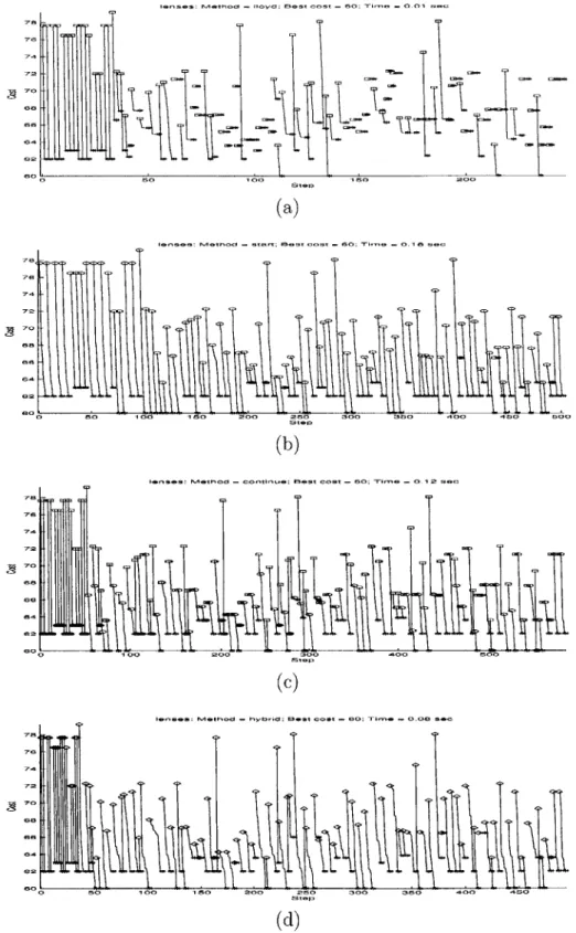
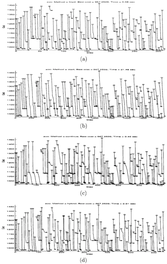
In addition to the final cost, the cost after each step that Cyclic Exchange applies negative-cost cycle to the solution and after each step that Lloyd's algorithm moves a single point are also recorded. These trails of costs will reveal the dynamics within an iteration of Cyclic Exchange and Lloyd's algorithm.

5.1.2 Results and Discussion

The final cost and time for Lloyd's algorithm and three versions of Cyclic Exchange are shown in Table 5.1. As a preliminary assessment, the program is run only on small-size datasets. In general, the time used by all versions of Cyclic Exchange is significantly more than the time used by Lloyd's algorithm, and the Cyclic Exchange get better costs in a few datasets.

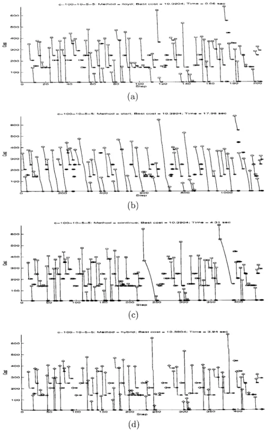
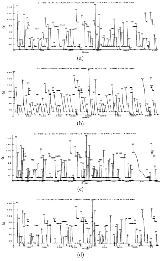
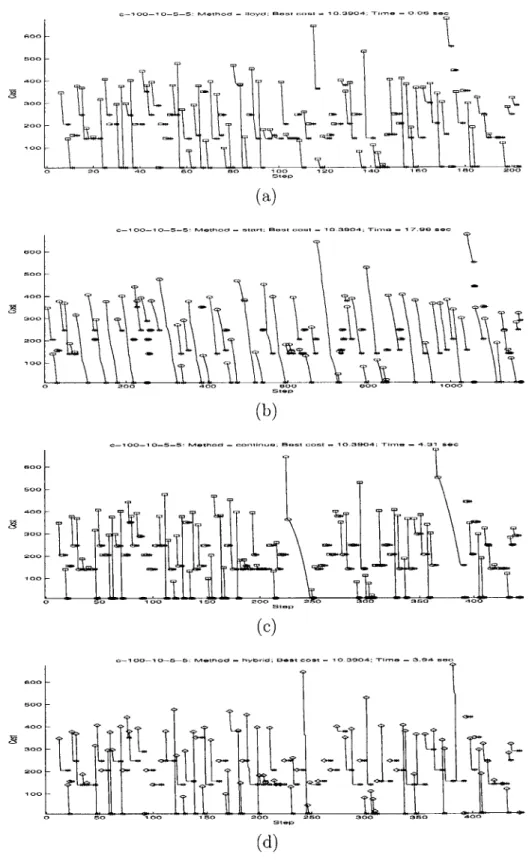
Figure 5-1 shows the costs over 100 iterations of Lloyd's algorthm and three ver-sions of Cyclic Exchange for dataset c-100-10-5-5, for which all verver-sions of Cyclic Exchange do not get better results. Figure 5-2 shows similar graphs for dataset m-100-10-5, for which all versions of Cyclic Exchange get better results. The graphs

(43)

Table 5.1: Comparison between Lloyd's algorihtm, Start Cyclic Exchange, Continue Cyclic Exchange, and Hybrid Cyclic Exchange. All methods run for 100 iterations.

Dataset k Final Cost Time (seconds)

Lloyd Start Continue Hybrid Lloyd Start Continue [Hybrid

c-100-3-5-5 53 3.5151e + 00 3.5151e + 00 3.5151e + 00 3.5151e + 00 0.05 28.37 5.63 5.83

c-100-5-5-5 53 3.8248e + 00 3.8248e + 00 3.8248e + 00 3.8248e + 00 0.05 24.68 4.94 5.95

c-100-10-5-5 53 1.0390e + 01 1.0390e + 01 1.0390e + 01 1.0390e + 01 0.06 17.96 4.31 3.94

c-100-20-5-5 53 1.9527e + 01 1.9527e + 01 1.9527e + 01 1.9527e + 01 0.09 20.43 4.28 5.11

c-200-3-5-5 53 7.0512e + 00 7.0512e + 00 7.0512e + 00 7.0512e + 00 0.09 331.49 94.27 40.37

c-200-3-10-5 53 1.0279e + 02 1.0279e + 02 1.0279e + 02 1.0279e + 02 0.09 370.01 37.98 35.94

c-200-5-5-5 53 1.9782e + 01 1.9782e + 01 1.9782e + 01 1.9782e + 01 0.10 164.68 18.24 24.28

c-200-5-10-5 53 1.7848e + 02 1.7848e + 02 1.7848e + 02 1.7848e + 02 0.09 179.20 14.06 12.50

c-200-10-5-5 53 1.8564e + 01 1.8564e + 01 1.8564e + 01 1.8564e + 01 0.12 218.18 16.98 20.70

c-200-10-10-5 53 6.3048e + 02 6.3048e + 02 6.3048e + 02 6.3048e + 02 0.10 130.80 16.31 13.18

c-200-20-5-5 53 6.1182e + 01 6.1182e + 01 6.1182e + 01 6.1182e + 01 0.17 148.14 30.63 38.02

c-200-20-10-5 53 1.6607e + 03 1.6607e + 03 1.6607e + 03 1.6607e + 03 0.15 123.89 8.53 11.76

m-100-3-5 53 3.0179e + 01 3.0179e + 01 3.0179e + 01 3.0179e + 01 0.05 56.05 7.58 4.45

m-100-5-5 53 9.6927e + 01 9.6927e + 01 9.6927e + 01 9.6927e + 01 0.05 37.54 8.32 5.72

m-100-10-5 53 5.2319e + 02 5.1164e + 02 5.1200e + 02 5.1200e + 02 0.10 26.64 8.51 6.00

m-100-20-5 53 3.3160e + 02 3.3160e + 02 3.3160e + 02 3.3160e + 02 0.10 200.83 6.24 5.20

m-200-3-5 53 3.3730e - 01 3.3730e - 01 3.3730e - 01 3.3730e - 01 0.11 290.85 29.12 36.23

m-200-5-5 53 3.3783e + 02 3.3783e + 02 3.3783e + 02 3.3783e + 02 0.11 324.85 33.08 24.18

m-200-10-5 53 1.5087e + 03 1.5082e + 03 1.5076e + 03 1.5084e + 03 0.31 774.08 81.74 120.61

m-200-20-5 53 1.7223e + 03 1.6912e + 03 1.6912e + 03 1.6912e + 03 0.19 372.21 47.36 25.78

covtype-100 53 2.9006e+03 2.8365e+03 2.8366e+03 2.8366e+03 0.29 121.28 49.15 39.17

glass 51 1.2391e + 03 1.2391e + 03 1.2391e + 03 1.2391e + 03 0.16 238.14 15.65 20.13

lenses 51 6.0000e+01 6.0000e+01 6.0000e+01 6.0000e+01 0.01 0.18 0.12 0.08

soybean 52 3.6714e + 02 3.6714e + 02 3.6714e + 02 3.6714e + 02 0.07 5.97 1.10 1.27

wine 51 1.2779e + 03 1.2779e + 03 1.2779e + 03 1.2779e + 03 0.12 833.00 17.16 19.14

(44)

(a)

c- 1 00-1 - - : M-hd..sat e t O - a390 ; -m --- /9 e

(b)

c-1 00-1 -5-5: Metho csts~e e --t O- Z3'O4; Trim- 4.3 1s

0 0 100 150 200 250 00 350

> 50 100 150 200 250 300 050 00

(d)

Figure 5-1: Dynamics During Iterations of Lloyd's Algorithm and Cyclic Exchange for Dataset c-100-10-5-5: (a) Lloyd's algorithm, (b) Start Cyclic Exchange, (c)

Continue Cyclic Exchange, (d) Hybrid Cyclic Exchange.

1 a -Q 100 laa Oa L- 0- -- 5 eh d-.iod;B s o . .9 4 Tm .6s Goo Soo 00 a00 000 100

(45)

(a)

-100-1 0-5: ~00 M -"O o E3- ~ S1 095i

-65s

20 00 a00 600 1 0

S 0 20 30 20 6 0 1 it00 10 a00

(d)

Figure~~0- 5-2: Dynamic Durin Itrtin of Lloyd's Algrih and5 Cyli Exhngo

Dataset m-7E001-:()Lodsagrtm(bStrCylcEcag,()oniu

Cyclic ExhneLd yrdCci xhne

(46)

points for Lloyd's algorithm, circles denote starting points for Cyclic Exchange, and asterisks denote the final costs for each iteration. For Hybrid Cyclic Exchange, di-amonds denote the starting point where Lloyd's algorithm and Cyclic Exchange are applied alternatively.

For both datasets, Start Cyclic Exchange gradually decrease the cost over many steps in each iterations. Since each step of Cyclic Exchange takes considerable amount of time, Start Cyclic Exchange takes much more time than Continue Cyclic Exchange, as shown in Table 5.1. Hybrid Cyclic Exchange gets the same costs for almost datasets as Continue Cyclic Exchange, and it also takes comparable time to Continue Cyclic Exchange.

For the datasets that all versions of Cyclic Exchange cannot obtain better solu-tions (e.g. c-100-10-5-5, as shown in Figure 5-1), each iteration of Continue Cyclic

Exchange consists of only one step - to verify that there is no negative-cost cycle

in the improvement graph. On the other hand, for some datasets (e.g. m-100-10-5, as shown in Figure 5-2), Cyclic Exchange is capable of finding more improvement upon Lloyd's algorithm. In this case, Continue Cyclic Exchange utilizes fast Lloyd's algorithm to bring down the cost significantly and uses slower Cyclic Exchange steps to decrease the cost further.

In addition to the longer running time, the final costs for Start Cyclic Exchange are no smaller than those for Continue Cyclic Exchange with an exception of dataset m-100-10-5 where the different is almost insignificant. This observation implies that using random starts for Cyclic Exchange is not preferable. Lloyd's algorithm can achieve the same amount of cost decreases in much less time. Applying Cyclic Ex-change only after Lloyd's algorithm has reached a local optimum seems more reason-able.

An apparent problem seen from the results above is the running time of all ver-sions of Cyclic Exchange. Cyclic Exchange uses 3 to 4 order of magnitudes more time than Lloyd's algorithm and yet obtains similar results. Although [2] sucessfully uses the subset-disjoing negative-cost cycle detection algorithm to perform neighborhood search on the capacitated minimum spaning tree problem (CMST), the same

(47)

algo-rithm seems inviable here. For CMST, [2] runs the program for 3600 seconds on the graph with 200 nodes. This degree of complexity is plausible for CMST, but it is not comparable to Lloyd's algorithm, which is very fast. Unless Cyclic Exchange can get a much lower cost than Lloyd's algorithm, it will not be a substitute for Lloyd's algorihtm. This problem leads us to try to increase the scalability of Cyclic Exchange via preclustering.

5.2 Cyclic Exchange with Preclustering

5.2.1 Methods

The results from the previous section suggest that Cyclic Exchange takes too long to be practical, no matter what type of initial solutions are used. In order to improve the scalability of cyclic exchange, we try to decrease the effective data size. [14] suggests that not all data are equally important. For example, data points that are very close together may be assumed to be in the same cluster. These data points can be preclustered and treated effectively as a single data point, which needs to be scaled appropriately when the cost is calculated.

In this section, we present our experiments on two kinds of preclustering: Two-point preclustering and Birch preclustering. For both experiments, we record final

cost, time, and effective data size after preclustering.

Two-point Preclustering

The first try on decreasing the effective data size is to group any two data points that are very close into a minicluster. The threshold for how close the two points in the minicluster should be is to be determined. The preclustered points will never be taken apart and will essentially be in the same cluster in every solution. A minicluster can be sufficiently described by the number of points in the minicluster and the vector sum of all points in the minicluster since the cost function in Eq. 2.2 involves only these two quantities. This description of a minicluster is similar to the clustering feature

Cyclic exchange neighborhood search technique for the K-means clustering problem