HAL Id: hal-02288755
https://hal-amu.archives-ouvertes.fr/hal-02288755
Submitted on 16 Sep 2019
HAL is a multi-disciplinary open access archive for the deposit and dissemination of sci-entific research documents, whether they are pub-lished or not. The documents may come from teaching and research institutions in France or abroad, or from public or private research centers.
L’archive ouverte pluridisciplinaire HAL, est destinée au dépôt et à la diffusion de documents scientifiques de niveau recherche, publiés ou non, émanant des établissements d’enseignement et de recherche français ou étrangers, des laboratoires publics ou privés.
Evaluation of Spin-Orbit Couplings with
Linear-Response Time-Dependent Density Functional
Methods
Xing Gao, Shuming Bai, Daniele Fazzi, Thomas Niehaus, Mario Barbatti,
Walter Thiel
To cite this version:
Xing Gao, Shuming Bai, Daniele Fazzi, Thomas Niehaus, Mario Barbatti, et al.. Evaluation of Spin-Orbit Couplings with Linear-Response Time-Dependent Density Functional Methods. Jour-nal of Chemical Theory and Computation, American Chemical Society, 2017, 13 (2), pp.515-524. �10.1021/acs.jctc.6b00915�. �hal-02288755�
Evaluation of spin-orbit couplings with
linear-response TDDFT, TDA, and TD-DFTB
Xing Gao†*, Shuming Bai‡, Daniele Fazzi†,
Thomas Niehaus§, Mario Barbatti‡*, Walter Thiel†*
†Max-Planck-Institut für Kohlenforschung, Kaiser-Wilhelm-Platz, D-45470, Mülheim an der Ruhr, Germany
‡Aix Marseille Univ, CNRS, ICR, Marseille, France
§Univ Lyon, Université Claude Bernard Lyon 1, CNRS, Institut Lumière Matière, F-69622, VILLEURBANNE, France
Abstract
A new versatile code based on Python scripts was developed to calculate spin-orbit coupling (SOC) elements between singlet and triplet states. The code, named PySOC, is interfaced to third-party quantum chemistry packages, such as Gaussian 09 and DFTB+. SOCs are evaluated using linear-response (LR) methods based on time-dependent density functional theory (TDDFT), the Tamm-Dancoff approximation (TDA), and time-dependent density functional tight binding (TD-DFTB). The evaluation employs Casida-type wave functions and the Breit-Pauli (BP) spin-orbit Hamiltonian with an effective charge approximation. For validation purposes, SOCs calculated with PySOC are benchmarked for several organic molecules, with SOC values spanning several orders of magnitudes. The computed SOCs show little variation with the basis set, but are sensitive to the chosen density functional. The benchmark results are in good agreement with reference data obtained using higher-level spin-orbit Hamiltonians and electronic structure methods, such as CASPT2 and DFT/MRCI. PySOC can be easily interfaced to other third-party codes and other methods yielding CI-type wave functions.
1 Introduction
Spin-orbit coupling (SOC) plays a fundamental role in spin-forbidden excited-state processes, such as intersystem crossing and phosphorescence. It is the core quantity to understand the phenomenology of many recent technological advances, including light emission in organic1-3 and in inorganic (transition metal)4-6 devices, or spin/charge transport in hybrid perovskite devices7. From a quantum-chemical standpoint, it is challenging to compute SOC elements effectively and accurately in such complex systems. Considering the increasing popularity of dynamics simulations for studying excited states8-15 and charge transport16 in spin-forbidden processes14,17-20, there is a vivid demand for new methods to efficiently evaluate SOC elements.
Motivated by this demand for efficiency, we focus on the computation of SOCs in the framework of DFT-based linear-response (LR) methods, in particular time-dependent density functional theory (TDDFT), the Tamm-Dancoff approximation to LR-TDDFT (denoted as LR-TDDFT/TDA or simply as TDA), and time-dependent density functional tight binding (TD-DFTB). The latter is an approximate TDDFT method with significantly reduced computational load.
In the past, two routes have been pursued to calculate SOCs in DFT-based methods: i) variational methods, and ii) perturbative methods.21 One of the earliest variational approaches involves the zeroth-order regular approximation (ZORA) Hamiltonian22-24, while later more accurate methods employ the exact two-component
(X2C) Hamiltonian25-27. By applying ZORA to the Dirac equation, relativistic DFT
methods were developed, in which SOC is naturally included in the two-component Hamiltonian22-24. Using this approach combined with LR-TDDFT and a non-collinear
exchange-correlation kernel28, SOC effects were explored through variational calculations29. We note that SOC effects are also taken into account naturally in time-dependent four-component relativistic density functional theory30,31. These methods are rigorous and of high quality, but also computationally very expensive, which is a serious limitation for the type of applications we have in mind.
The second route, based on perturbative approaches, has been broadly adopted not only for the ZORA Hamiltonian32 (as implemented in the quantum chemistry packages ADF29,32,33 and TURBOMOLE34,35), but also for other SOC Hamiltonians such as the Breit-Pauli (BP) operator. There have been two main developments in this area: 1) formally exact response theory (RP), which obtains SOCs from the residue of the response function without the need for explicit electronic states36,37; 2) evaluation of SOCs directly from DFT-based excited-state wave functions. Such wave functions can be built either through a multi-configuration (MR) configuration interaction (CI) formalism in Kohn-Sham space (as done in DFT/MRCI38) or through approximate
CI-like wavefunctions derived from linear-response time-dependent eigenvectors. SOC calculations using DFT/MRCI wave functions are discussed in Refs.39,40, while those using approximate CI-like wave functions, either based on Casida’s41 or Sternheimer’s42,43 formalism, are discussed in Refs.44-46. In the framework of the X2C
Hamiltonian, spin-adapted TDDFT has been combined with a perturbational SOC treatment to evaluate the fine-structure splittings of excited states of open-shell systems47.
Moving beyond specific quantum chemistry programs, Chiodo, Russo, and co-workers have recently developed a code to compute SOCs, called MolSOC, which works as a general interface that can be adapted to third-party programs.48-50 In this
approach, one can choose an arbitrary program and use its output directly to calculate SOC elements, without relying on a specific SOC implementation in that program. MolSOC uses approximate CI-like wave functions. It has been successfully tested for several systems49,51,52. However, there are two shortcomings in MolSOC: one is the rather low flexibility of the input/output (I/O) interface written in FORTRAN; the other one is that only the main terms in CI-like wave functions are considered and an additional molecular orbital shift process (the so-called alteration procedure) is needed to evaluate the SOC between CI wave functions, which limits the accuracy and efficiency of the code.
The present SOC implementation is based on the multiple-interface idea of MolSOC, but benefits from the flexibility of a script language. In the computational chemistry community, such script languages are often used, for example Tcl/Tk in Chemshell53, Perl in Newton-X54, and Python in SHARC55. We have adopted Python scripting to deal with the I/O interface in PySOC. The formally exact RP theory is not well suited for our multiple-interface philosophy, and therefore, to balance flexibility, accuracy, and efficiency, we have adopted the wave function approach to describe the excited states, including all CI terms in TDDFT via Casida’s Ansatz, which also eliminates the need of using the alteration procedure. Reconstructed Casida-type wavefunctions are in principle capable of producing the exact LR-TDDFT matrix elements for one-body operators between ground and excited states56 and between pairs of excited states57.
In this article we present the implementation of our interface code called PySOC. In the first version, PySOC is able to evaluate SOCs between singlet and triplet states, using the single-particle BP operator with an effective charge approximation. SOCs can be computed either between ground and excited states, or between excited states. The current version of PySOC makes use of Casida-type wave functions in the framework of LR-TDDFT, TDA, and TD-DFTB, and imports the SOC integrals from MolSOC. The data I/O is handled with Python scripts, while the numerical evaluations are carried out by a FORTRAN code. PySOC has been initially interfaced to Gaussian 0958 (TDDFT59, TDA60) and to DFTB+61,62 (TD-DFTB63).
In the next sections, we describe the basic theory underlying the SOC computation in PySOC, the implementation, and benchmarks of the computed SOC values for small to medium-size organic compounds.
2 Implementation
2.1 Theory
2.1.1 Hamiltonian
Conceptually we start from the BP operator, which contains one- and two-electron terms resulting from the interaction of the electron spin magnetic moment with the magnetic field generated by the motion of the electron around the nucleus or other electrons.21 In the current version of PySOC, we have implemented only a single-electron effective operator with an effective charge approximation to evaluate SOCs.
64-68 This approximate Hamiltonian is expressed as67-69
2 2 2 3 ˆ ˆ ˆ ˆ, 2 el A el N N N eff eff i SOC i i i i i i i i e e r H Z m c r
r p s
l s (1) where
2 2 2 3 2 A e N e i i ff Z e r m c r
is a radial function, Zeff is the effective charge for nucleus , ˆli ri piis the orbital angular momentum operator for electron i, andˆi
s is the spin angular momentum operator.
In second quantization notation the single-particle operator can be written as70
ˆˆ ˆ ˆ ˆˆ
† ˆ , p x e x y y z z q p ff so p q q r l s l s l a H s a
(2)with the two-component spinor q q. Here denotes a Kohn-Sham (KS) q orbital, ,
,
, and and denote spin-up and spin-down, respectively. Introducing the Pauli matrices for ˆs,0 1 0 1 0 1/ 2 , 1/ 2 , 1/ 2 , 1 0 0 0 1 x y z i s s s i (3)
† † † † † † ˆ 1 / 2 , ˆ 1 / 2 , ˆ 1 / 2 , p q p q p x x so pq pq y y so pq pq z z q p q p q p so pq q pq H h a a a a H i h a a a a H h a a a a
(4)where the creation {a†p...} and annihilation {aq...}operators obey the commutation relation
a†p,aq
pq . The matrix element hdpq of the SOC Hamiltonian betweenKS orbitals is defined as
ˆ ,
, y, z .
p d pq q d h r l d x (5) 2.1.2 Electronic statesThe closed-shell ground state S0, constructed from KS orbitals is denoted as KS . The
action of an excitation operator70 on S0 generates singly excited singlet configurations
Sa
i and triplet configurations T , b j s m:
† † † † † † 1/2 1,1 1, 1 1/2 1,0 S 2 K , , , S T KS T K 2 . S T KS a i a i a i b j b j b j b j b j j b b j a a a a a a a a a a a a (6)In these equations, s and m denote spin angular momentum and magnetic quantum
numbers, while
a b c, , ,
and
i j k, , ,
represent virtual and occupied orbitals. Adopting Casida’s wave function ansatz41 in the framework of collinear LR-TDDFT44, the Ith excited state is given by, ia a I I i ia C
(7)with CIia NI1/ 2
X Y
iaI , where
X Y
I denotes the coefficient vector for the Ith excitation in Casida’s equations. The term NI
X Y
I X Y
I is introduced to ensure normalization. Without it, normalization is satisfied only for TDDFT with functionals without any Hartree-Fock exchange. A critical discussion of the approximations implied by Casida’s ansatz can be found in refs71,72. Additionally, wenote that, for collinear LR-TDDFT, only the triplet with m = 0, TJ 1,0, can be obtained directly, and the other two components ( TJ 1, 1 ) are generated approximately from the
same ground state44.
2.1.3 Evaluation of the SOC matrix elements
With the definition of the Hamiltonian and the electronic states in equations (2) and (7), the SOC matrix elements between triplet states and excited singlet states can be evaluated by applying Wick’s theorem73,
† 1,1 † 1, 1 1,1 † † 1,0 ˆ S T 1 / 2 2 1 / 2 2 , ˆ ˆ S T S T , ˆ S T 1 / 2 1 / 2 . ia ja x y I so J I J ji ji ija ia ib x y I J ab ab abi I so J I so J ia ja z ia ib z I so J I J ji I J ab ija abi H C C h ih C C h ih H H H C C h C C h
(8)The SOC elements between triplet states and the closed-shell singlet ground state are
0 1,1 0 1, 1 0 1,1 0 1,0 ˆ S T 1 / 2 , ˆ ˆ S T S T , ˆ S T 1 / 2 . jb x y so J T jb jb jb so J so J jb z so J T jb jb H C h ih H H H C h
(9)It should be noted that the Gaussian 09 code adopts the normalization
†
0.5
I I
X Y X Y in closed-shell TDDFT and TDA, and hence one needs to multiply the right-hand side of equation (6) by 2to ensure normalization to unity;
equations (8) and (9) need to be modified accordingly. After the expansion of the KS orbitals in a basis set
, ,...
, with q cq
, the SOC matrix element defined in equation (5) can be evaluated as† , N d d pq p q h c h c
(10)in terms of atomic integrals hd
r lˆd ,d
x y z, ,
.The singlet-triplet SOC values (SK = S0 or SI) reported in the following are defined as
2 2 2 1,1 1, 1 1,0 1 ˆ ˆ ˆ SOC S T + S T + S T . 3 K Hso J K Hso J K Hso J (11) 2.2 PySOC program
Figure 1. PySOC program flowchart.
As illustrated in Figure 1, there are three main functional modules in PySOC: 1) the user control and parameter definition module (init.py); 2) the data exchange and transformation module (soc.py); 3) the calculation module (SOC_TD). The former two are implemented with Python scripts, while the third one is coded in FORTRAN.
The third-party quantum chemistry packages Gaussian 09 and DFTB+ have been interfaced to PySOC to provide KS orbitals, orbital energies, excitation energies, and linear-response eigenvectors from TDDFT, TDA, and TD-DFTB. Due to the modularity and flexibility of Python scripts, the interface can be easily extended to other packages and methods.
The atomic integral in equation (10) is obtained separately from the MolSOC code48,50. When Gaussian 09 is called, contracted Gaussian-type orbitals (c-GTOs) are usually chosen for the electronic structure calculation. However, the order of the components of d and f orbitals in Gaussian 09 is different from that in MolSOC. Therefore, the computed matrix of atomic integrals from MOLSOC is blocked and transformed to match the order of Gaussian 09. Technical details for the block matrix transformation (BMT) are provided in the Supporting Information, Section S1.
In the case of DFTB+, we need more steps to process the atomic integrals in the interface. First, the spherical Slater-type orbitals (STOs) used in DFTB+ are fitted with c-GTOs. Then, using the resulting contraction coefficients and exponents as input to MolSOC, the atomic integrals are computed. For this purpose, the original MolSOC code50 had to be modified and adapted to the fitted GTOs. In the last step, the atomic integrals in the c-GTO basis are transformed back to the STO basis. Again the BMT technique is applied. Details on basis sets fitting and BMT are included in the Supporting Information, Sections S2 and S3.
3 Computational details
Molecular structures were either obtained directly from the literature or optimized for the electronic state of interest at the (TD) DFT level using Gaussian 09. The DFT optimization employed the hybrid density functionals PBE074 or B97XD75 combined with the standard split-valence triple-zeta basis sets TZVP76,77. At the optimized structures, electronic excited-state properties were calculated with TDDFT and
LR-TDA (Gaussian 09) or with LR-TD-DFTB (DFTB+). In the DFTB+ calculations, the Slater-Koster parameter set mio-1-178,79 was applied.
SOC matrix elements were evaluated with PySOC, which calls the MolSOC code to calculate the atomic integrals. Parameters for the effective charge in the operator for the atomic integrals were taken from the MolSOC code69 without further optimization.
For comparison purposes, the Dalton program80 was used to compute SOCs within the mean-field approximation (AMF) or with the full BP operator from the residues of linear or quadratic RP37, with the reference states being calculated at the
DFT/cc-pVTZ81/(CAM)-B3LYP82-85 level.
Also for the sake of comparison, MS-CASPT286 calculations were done with MOLCAS 887 for thymine and its thio-derivatives. The active space was composed of 14 electrons in 10 orbitals (2n, 5, 3*) using the ANO-RCC-VTZP basis set, which accounts for relativistic effects88. Independent calculations were performed for the singlet and triplet manifolds, with the CASSCF treatment averaged over 5 states in each case. The standard ionization potential-electronic affinity (IPEA) shift was adopted throughout. For SOC calculations, the Douglas-Kroll (DK) Hamiltonian was used89 and the SOC operator was approximated by a one-electron effective operator64, which
retains all multicenter SOC terms (contrary to the AMF approximation21,65).
The PySOC results were also compared with DFT/MRCI data taken from literature (see Section 4), which provide SOCs computed with the use of the BP AMF Hamiltonian.
4 Results and Discussion
Figure 2. Model structures of the investigated molecules: a) formaldehyde, b) acetone, c) 2-thiothymine (2tThy), d) thymine (Thy), e) 4-thiothymine
(4tThy), f) 2,4-thiothymine (2,4tThy), g) 7H-furo[3,2-g][1]benzopyran-7-one
(psoralenOO), h) 7H-thiopyrano[3,2-f][1]benzofuran-7-one (psoralenOS), i)
2H-thieno [3,2-g] [1] benzopyran-2-one (psoralenSO), j) boron-dipyrromethene
(BODIPY).
Results are given for the molecules shown in Figure 2. They are presented in six sections:
1) Analysis of basis set effects using 2tThy (Figure 2c, Section 4.1);
2) Analysis of density functional effects also for 2tThy (Figure 2c, Section 4.2);
3) SOC in formaldehyde and acetone (Figure 2a,b, Section 4.3.1);
4) SOC in thymine derivatives (Figure 2d-f, Section 4.3.2);
The following abbreviations are used to label the methods for SOC computation: BP1e-eff for the single-electron BP operator with an effective charge approximation (the method employed in PySOC); BP1e-mf for the BP operator with the AMF approximation (used in SPOCK and Dalton); BP1,2e for the full BP operator including one- and two-electron contributions (used in Dalton); DK1e-eff for the DK Hamiltonian with an effective one-electron approximation (used in MOLCAS).
4.1 Basis set effects
Table 1. SOCs for 2tThy: Basis set effects at the TDDFT/B3LYP/BP1e-eff level.
SOC (cm-1) (TD-B3LYP) S0/T1 S0/T2 S1/T1 S1/T2 cc-pVDZ 91 134 129 71 aug-cc-pVDZ 89 130 125 74 cc-pVTZ 91 138 134 73 TZVP 97 143 137 78
The SOC results for 2tThy with different basis sets are listed in Table 1. The calculations were done at the S1 minimum. Four basis sets, cc-pVDZ, aug-cc-pVDZ,
cc-pVTZ, and TZVP, were chosen to calculate three excited states S1, T1, and T2 to
cover n→* and →* transitions within TDDFT/B3LYP.
Going from cc-pVDZ to cc-pVTZ, the calculated excitation energies vary by less than 0.02 eV (Table S1, Supporting Information). The computed SOC values agree within 13 cm-1 for all basis sets (Table 1). Inclusion of diffuse functions (from cc-pVDZ
to aug-cc-pVDZ) reduces the couplings for S0/T1, S0/T2, and S1/T1, but increases them
for S1/T2. The SOCs tend to increase slightly when moving from a double- (cc-pVDZ)
via a triple- (cc-pVTZ) to the TZVP basis. Overall the SOCs are rather insensitive to the chosen basis set, and we will thus only use the TZVP basis from now on.
4.2 Density functional effects
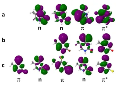
Figure 3. The dominant active KS orbitals in S1, T1, and T2 for 2tThy. HOMO-1 and HOMO have strong / n mixing; LUMO and LUMO+1 are *.
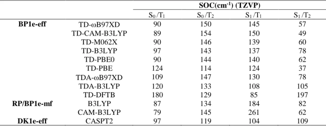
Table 2. SOCs for 2tThy: Dependence on the choice of density functional at the TDDFT and TDA levels for the BP1e-eff approach (PySOC). Results from RP/BP1e-mf (Dalton) and
CASPT2/DK1e-eff (MOLCAS) are provided as well.
SOC(cm-1) (TZVP) S0 / S0 / S1 / S1 / BP1e-eff TD-B97XD 90 150 145 57 TD-CAM-B3LYP 89 154 150 49 TD-M062X 90 146 139 60 TD-B3LYP 97 143 137 78 TD-PBE0 90 144 140 62 TD-PBE 124 114 124 37 TDA-B97XD 109 147 130 78 TDA-B3LYP 120 133 108 105 TD-DFTB 180 129 85 197 RP/BP1e-mf B3LYP 87 134 184 82 CAM-B3LYP 79 145 261 62 DK1e-eff CASPT2 97 119 104 109
Table 2 lists SOCs for 2tThy computed with different density functionals. Several types of density functionals were applied in TDDFT calculations, namely one pure GGA functional (PBE90), two hybrid GGA functionals (B3LYP and PBE0), one hybrid meta-GGA functional (M062X91), and two long-range corrected (LC) functionals (CAM-B3LYP and B97XD). The (CAM-B3LYP and B97XD functional were also used with TDA60. For comparison, SOC results are given in Table 2 also at the RP/BP1e-mf level using B3LYP and CAM-B3LYP, and at the DK1e-eff level using CASPT2. The main
KS orbitals contributing to S1, T1, and T2 are shown in Figure 3; they are similar for all
functionals.
With the exception of PBE, all functionals predict the same energetics within 0.2 eV (Table S2, Supporting Information). It is worth mentioning that the KS orbital energy gap for the dominant transition in each state is strongly affected by the functional and decreases in the following order: LC > hybrid > pure (data not shown).
Examining the results in Table 2, we see that SOCs computed with BP1e-eff (PySOC) and TDDFT using hybrid or range-separated functionals are in very good agreement with each other. The maximum deviation observed in this subset of data is 18 cm-1, but most of results differ much less. Going within TDDFT from hybrid to pure functionals (compare, for instance, TD-PBE0 and TD-PBE) the changes are larger, about 30 cm-1. Comparing the TDDFT and TDA results with the same functional, there are deviations of about 20 to 30 cm-1.
The differences between TDDFT and TD-DFTB results are much larger. By construction, TD-DFTB should be closest to TD-PBE. However, comparing these two data sets, the SOC deviation is 66 cm-1 for S0/T1, 15 cm-1 for S0/T2, -33 cm-1 for S1/T1,
and 160 cm-1 for S
1/T2. These large discrepancies seem to be connected to a different
description of the excited states in the two methods. The excited states of 2tThy are strongly multi-configurational in TD-PBE (and TDDFT in general), with important contributions from two determinants, whereas they are basically mono-configurational with TD-DFTB. To avoid misunderstandings, we note that the ground state is still well described by a single reference determinant, for all cases and methods.
We can get some insight on the influence of the approximation for the spin-orbit operator by comparing the B3LYP and CAM-B3LYP results computed with effective charges (BP1e-eff) and with the mean-field scheme (BP1e-mf), the latter being the higher level. There is reasonable agreement between the two sets of data, with deviations of about 10 cm-1 in most cases, except for the S
1/T1 SOC, for which the
The SOCs from TDDFT/BP1e-eff and CASPT2/DK1e-eff differ by about 30 cm-1 (TD-B3LYP). Curiously, the agreement between TDA and CASPT2 is slightly better, with deviations of about 20 cm-1 (TDA-B3LYP).
Figure 4. SOCs for 2tThy: Dependence on the range separation parameter within TDDFT/LC-BLYP.
To explore the influence on long-range corrections, we plot SOCs for 2tThy computed with LC-BLYP92 as a function of the range-separation parameter (Figure 4). The
SOCs for all transitions depend strongly on . For S0/T2 and S1/T1, the SOC increases
with , while it shows the opposite behavior for S0/T1 and S1/T2. The maximum
variation over the domain is about 80 cm-1, in the case of S1/T2. This dependence of the
SOC on is relevant because is often tuned for better performance in a given application93. For LC-BLYP, even the default value differs in different programs:
Gaussian 09, = 0.47 a0-1; Gamess94, = 0.33 a0-1; an empirical parameterization95of
4.3 Benchmark calculations
4.3.1 Formaldehyde and acetone
Figure 5. The dominant active molecular orbitals in S1, T1, and T2 for (a) formaldehyde and (b) acetone. HOMO-1 and HOMO are and n, respectively;
LUMO is *.
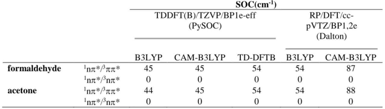
Table 3. SOCs for formaldehyde and acetone at the TDDFT/TZVP/(CAM-)B3LYP and TD-DFTB levels compared with RP/DFT/cc-pVTZ/(CAM-)B3LYP results.
SOC(cm-1) TDDFT(B)/TZVP/BP1e-eff (PySOC) RP/DFT/cc-pVTZ/BP1,2e (Dalton)
B3LYP CAM-B3LYP TD-DFTB B3LYP CAM-B3LYP
formaldehyde 1n*/* 45 45 54 54 87
1n*/3n* 0 0 0 0 0
acetone 1n*/* 44 45 54 54 88
1n*/3n* 0 0 0 0 0
Formaldehyde and acetone were optimized in the ground state using DFT/TZVP/B97XD. At this geometry, vertical excitation energies were calculated and the dominant excitations were identified (Table S3, Supporting Information). Both
TD-DFTB as well as TDDFT with B3LYP and CAM-B3LYP were used. The relevant active frontier orbitals are shown in Figure 5. For both molecules, independent of the method, S1 and T1 are n→* states, while T2 is a →* state.
Table 3 lists the SOCs computed at the BP1e-eff level (PySOC) together with those computed at the BP1,2e level (Dalton). Qualitatively, the PySOC calculations clearly differentiate strong SOCs (1n*/*) from weak ones (1n*/3n*) in these systems, consistently with the El-Sayed rules97. Looking more quantitatively at the B3LYP data, the PySOC calculations tend to underestimate the SOC by about 10 cm-1
for strong couplings compared with the Dalton results. Curiously, TD-CAM-B3LYP and TD-B3LYP give basically the same results at the BP1e-eff level, but deviations of 30 cm-1 at the RP/BP1,2e level (similar as in the case of 2tThy, see Table 2). The results from TD-DFTB are comparable to those obtained from long-range corrected functionals. Similar trends with regard to the density functional are found when using the Dalton code, in which the SOCs are calculated with the full BP Hamiltonian.
4.3.2 Thymines
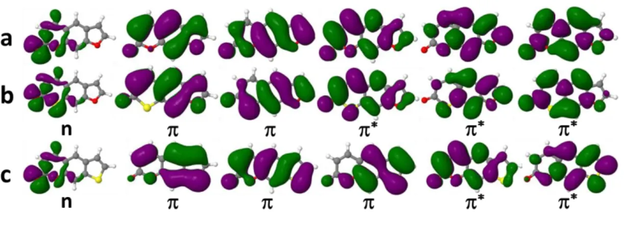
Figure 6. Dominant active molecular orbitals in S1, T1, and T2 for thymines: a) Thy, b) 4tThy, c) 2,4tThy. The and n orbitals have different order in different
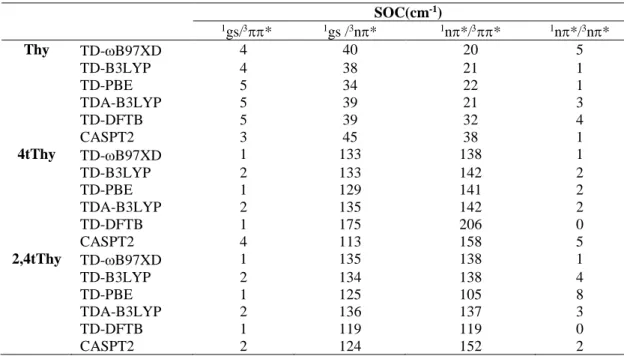
Table 4. SOCs for Thy, 4tThy, and 2,4tThy computed with TDDFT/TZVP/ (B3LYPB97XD, PBE), TDA/TZVP (B3LYP), and TD-DFTB at the BP1e-eff level,
compared to SOCs from CASPT2 at the DK1e-eff level. For 2tThy, see Table 2.
SOC(cm-1) 1gs/* 1gs /3n* 1n*/* 1n*/3n* Thy TD-B97XD 4 40 20 5 TD-B3LYP 4 38 21 1 TD-PBE 5 34 22 1 TDA-B3LYP 5 39 21 3 TD-DFTB 5 39 32 4 CASPT2 3 45 38 1 4tThy TD-B97XD 1 133 138 1 TD-B3LYP 2 133 142 2 TD-PBE 1 129 141 2 TDA-B3LYP 2 135 142 2 TD-DFTB 1 175 206 0 CASPT2 4 113 158 5 2,4tThy TD-B97XD 1 135 138 1 TD-B3LYP 2 134 138 4 TD-PBE 1 125 105 8 TDA-B3LYP 2 136 137 3 TD-DFTB 1 119 119 0 CASPT2 2 124 152 2
The photochemistry of thymine and its thio-derivatives has been intensely studied both experimentally and theoretically.98-104The energies and the main orbital contributions of the lowest singlet 1n* state and the lowest triplet 3* and 3n* states obtained with TDDFT, TDA, TD-DFTB, and CASPT2 are summarized in Table S4 of Supporting Information. These values are computed at the S1 minimum geometry. The frontier
orbitals contributing to these excited states are shown in Figure 6. They are always of the same type, but the order of the states may change depending on the method: 1n* is S2 for TD-B3LYP, TD-B97XD, and CASPT2, but S1 for all other methods. For all
methods, 3* is T
1 and 3n* is T2.
Table 4 lists the SOCs for these molecules (for 2Thy, Table 2). Note that there is a striking difference between Thy, 4t-Thy, and 2,4tThy, on the one hand, and 2tThy on the other. While the SOCs in the former conform to the El-Sayed rules, this is not true in the latter. The reason is that the S1 minimum of 2tThy is strongly distorted
out-of-plane, with concomitant mixing of n and orbitals, while it is planar for the other three molecules.
It is obvious from Table 4 that all DFT-based results can qualitatively discriminate between strong (1gs/3n*, 1n*/*) and weak (1gs/*, 1n*/3n*)
couplings. All methods also correctly show the enhancement of the strong couplings upon single or double thio-substitution in thymine. More quantitatively, for weak couplings, the DFT-based SOCs computed at the BP1e-eff level agree with the CASPT2 SOCs computed at the DK1e-eff level to within less than 10 cm-1. For strong couplings, there are larger variations depending on the method and functional. The mean square-root deviation (RMSD) from CASPT2 is 15 cm-1 for B3LYP and
TD-B97XD. It increases to 23 cm-1 for TD-PBE and further to 35 cm-1 for TD-DFTB.
4.3.3 Psoralens
Figure 7. The dominant active molecular orbitals in S1-S3, T1-T5(T6) for psoralens: a) psoralenOO, b) psoralenOS, and c) psoralenSO. The order of and
n depends on the method; the lowest unoccupied orbitals are *.
Table 5. SOCs for psoralens computed with TDDFT (B3LYP and B97XD) and TD-DFTB at the BP1e-eff level compared to SOCs computed with DFT/MRCI at the BP1e-mf level. Some
transitions between adiabatic states were reordered to match the diabatic character in the same
row. The reordering is indicated in parentheses.
SOC(cm-1) TD-B3LYP TD-B97XD TD-DFTB DFT/MRCIa psoralenOO S0/T1 1 1 0 (S0/T3) 0 S0/T4 43 48 (S0/T5) 32 (S0/T2) 50 S1/T1 1 1 0 (S2/T3) 0 S1/T2 0 1 0 (S2/T1) 0 S1/T3 0 0 0 (S2/T4) 0 S1/T4 8 9 (S1/T5) 12 (S2/T2) 10 S3/T1 19 15 16 (S1/T3) 28 psoralenOS S0/T1 1 1 0 (S0/T3) 0 S0/T4 70 72 75 (S0/T2) 78 S1/T1 0 1 0 (S2/T3) 0 S1/T2 0 0 0 (S2/T1) 0 S1/T3 0 0 1 (S2/T4) 0 S1/T4 37 35 62 (S2/T2) 36 S2/T1 10 7 26 (S1/T3) 11 psoralenSO S0/T1 0 1 1 (S0/T3) 0 S0/T5 42 47 (S0/T6) 30 (S0/T2) 49 S1/T1 1 1 1 (S2/T3) 0 S1/T2 0 0 0 (S2/T1) 0 S1/T3 0 0 1 (S2/T4) 0 S1/T5 4 7 (S1/T6) 5 (S2/T2) 6 S3/T1 16 14 23 (S1/T3) 26 a. Original data from ref.105 and recalculated for the total SOCs.
Psoralen and its thio-derivatives resulting from intracyclic substitution of oxygen by sulfur have been studied theoretically by Tatchen et al.105 using DFT/MRCI and by Chiodo and Russo51 using TDDFT. To further test the performance of PySOC, we
studied the excited-state properties of these compounds at the TDDFT/TZVP (B3LYP and B97XD) and TD-DFTB levels. The results are listed in Table S7 of Supporting Information. They refer to ground-state geometries optimized at the PBE0/TZVP level. The dominant KS orbitals are plotted in Figure 7.
The computed SOCs for the psoralen systems are listed in Table 5. Some of the entries had to be reordered since the different methods sometimes predict a different sequence of the electronic states. After taking this into account, the SOCs obtained from PySOC (BP1e-mf level) compare well with the DFT/MRCI results from SPOCK105
(BP1e-mf level). For weak SOCs, the calculated SOCs differ by less than 1 cm-1. For the stronger SOCs, the RMSDs relative to DFT/MRCI is around 7 cm-1 for TDDFT/B3LYP and TDDFT/B97XD, and less than 15 cm-1 for TD-DFTB.
4.3.4 BODIPY
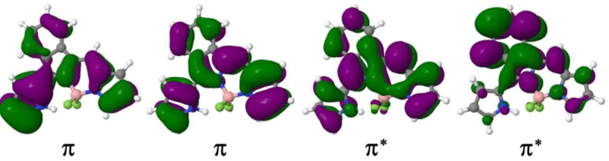
Figure 8. The dominant active molecular orbitals in S1, T1, T2 for BODIPY: and *
Table 6. SOCs for BODIPY computed with TDDFT/TZVP/(CAM-)B3LYP at the BP1e-eff level (PySOC) compared to SOCs computed with RP/DFT/cc-pVTZ/(CAM-)B3LYP at the
BP1e-mf level (Dalton).
SOC(cm-1)
TDDFT/TZVP/BP1e-eff RP/DFT/cc-pVTZ/BP1e-mf
B3LYP CAM-B3LYP B3LYP CAM-B3LYP
BODIPY S0/T1 1 1 1 1
S1/T1 0 0 0 0
S1/T2 0 0 0 0
The BODIPY molecule was re-optimized in the ground state with DFT/TZVP/B97XD starting from the initial structure in ref.106. The TDDFT vertical excitation energies computed with B3LYP and CAM-B3LYP for the S1, T1, and T2
states are reported in Table S8 of Supporting Information along with the dominant excitations. The relevant frontier orbitals are shown in Figure 8. They are of character and delocalized. SOCs for S0/T1, S1/T1 and S1/T2 transitions are reported in Table 6. All
4.4 Overall assessment of the SOC data
Figure 9. Plot of all SOCs calculated with PySOC versus reference data obtained from CASPT2 (MOLCAS), RP/B3LYP (DALTON), and DFT/MRCI
(SPOCK) as reported in this work.
Figure 9 shows a plot of the SOCs computed with TDDFT, TDA, and TD-DFTB in PySOC (for all molecules considered in this work) against those computed with CASPT2 (DK1e-eff with MOLCAS), RP/B3LYP (BP1,2e or BP1e-mf with Dalton),
and DFT/MRCI (BP1e-mf with SPOCK). This graph provides a global overview of the available data. The main features are:
1) BP1e-eff SOCs computed with TDDFT and TDA using either hybrid or LC functionals are in good agreement (<20 cm-1) with the reference data.
2) SOCs smaller than 1 cm-1 are predicted to be very small by most of the methods, usually within about ±1 cm-1 of the reference data.
3) For SOCs above 100 cm-1, the dispersion of the data tends to increase. The worst results were obtained for TD-PBE and TD-DFTB, which are both based on pure functionals: they have maximum deviations of nearly 100 cm-1.
5 Conclusions
We present a new program, named PySOC, to calculate spin-orbit couplings (SOC) elements. It is designed as a general interface. In its first version, PySOC is interfaced to Gaussian 09 and DFTB+ to compute SOCs based on linear-response TDDFT, TDA, and TD-DFTB. The method makes use of Casida-type approximate wave functions and of an effective-charge approximate BP Hamiltonian. Atomic integrals are obtained from the MolSOC code with modified interfaces for handling Slater- and Gaussian-type basis sets.
The SOC results from PySOC are validated for more than ten organic molecules, by comparing them to reference data obtained from CASPT2, DFT response theory, and DFT/MRCI calculations using a variety of approximate spin-orbit Hamiltonians. We find that the methods currently implemented in PySOC predict SOC values for weak couplings very well (deviations of ca. 1 cm-1) and give qualitatively correct results for strong couplings (with deviations that depend on the method, density functional, and density functional parameterization). Generally, the performance follows the order: pure < hybrid ~ LC functionals; and TD-DFTB < TDA < TDDFT. In the case of separated functionals, the predicted SOC values strongly depend on the range-separation parameter. The initial linear response calculation is typically the
computational bottleneck of SOC evaluations. TD-DFTB often deviates strongly from the higher-level methods, but may still be useful in practice for the treatment of large molecular systems since it correctly predicts general trends.
The accuracy and applicability of the SOCs obtained with PySOC is limited by two main approximations, namely: 1) the SOCs are obtained in a perturbative way and the assigned excited state is represented by a CI-like Casida-type wave function in collinear TDDFT, TDA, and TD-DFTB; and 2) the approximate single-electron Hamiltonian depends on effective charges.
To add further functionality to PySOC, we are actively exploring a series of new developments, including 1) extension of the interface beyond DFT-based methods to deal with coupled-cluster and algebraic-diagrammatic construction methods107; and 2) extension to mean-field BP Hamiltonians64,65. Other future enhancements will address the computation of intersystem crossing rates, phosphorescence rates, spectra, and dynamics.
Author information
Corresponding authors* E-mails: XG: [email protected]; MB: [email protected]; WT: [email protected].
Acknowledgments
XG thanks the Max-Planck-Gesellschaft for a postdoctoral research fellowship. SB and MB are grateful for support by the A*MIDEX grant (n° ANR-11-IDEX-0001-02) and the project Equip@Meso (ANR-10-EQPX-29-01), both funded by the French Government “Investissements d’Avenir” program. The authors thank Prof. Sandro Chiodo for discussions. XG thanks Shengfa Ye for helpful discussions.
Supporting Information Available
Block matrix transformation; STO fitting; excited state energies; Cartesian coordinates. This information is available free of charge via the Internet at http://pubs.acs.org/.
References
(1) Uoyama, H.; Goushi, K.; Shizu, K.; Nomura, H.; Adachi, C. Nature 2012, 492, 234-238. (2) Goushi, K.; Yoshida, K.; Sato, K.; Adachi, C. Nat. Photonics 2012, 6, 253-258.
(3) Minaev, B.; Baryshnikov, G.; Agren, H. Phys. Chem. Chem. Phys. 2014, 16, 1719-1758. (4) Eng, J.; Gourlaouen, C.; Gindensperger, E.; Daniel, C. Acc. Chem. Res. 2015, 48, 809-817. (5) Zhang, W.; Alonso-Mori, R.; Bergmann, U.; Bressler, C.; Chollet, M.; Galler, A.; Gawelda, W.; Hadt, R. G.; Hartsock, R. W.; Kroll, T. Nature 2014, 509, 345-348.
(6) Auböck, G.; Chergui, M. Nat. Chem. 2015, 7, 629-633.
(7) Zhang, C.; Sun, D.; Sheng, C. X.; Zhai, Y. X.; Mielczarek, K.; Zakhidov, A.; Vardeny, Z. V.
Nat. Phys. 2015, 11, 427-434.
(8) Kilina, S.; Kilin, D.; Tretiak, S. Chem. Rev. 2015, 115, 5929-5978. (9) Tully, J. C. J. Chem. Phys. 2012, 137, 22A-301A.
(10) Barbatti, M. WIREs Comput. Mol. Sci. 2011, 1, 620-633.
(11) Akimov, A. V.; Neukirch, A. J.; Prezhdo, O. V. Chem. Rev. 2013, 113, 4496-4565. (12) Wang, L.; Long, R.; Prezhdo, O. V. Annu. Rev. Phys. Chem. 2015, 66, 549-579. (13) Tavernelli, I. Acc. Chem. Res. 2015, 48, 792-800.
(14) Eng, J.; Gourlaouen, C.; Gindensperger, E.; Daniel, C. Acc. Chem. Res. 2015, 48, 809-817. (15) Thiel, W. WIREs Comput. Mol. Sci. 2014, 4, 145-157.
(16) Wang, L.; Prezhdo, O. V.; Beljonne, D. Phys. Chem. Chem. Phys. 2015, 17, 12395-12406. (17) Persico, M.; Granucci, G. Theor. Chem. Acc. 2014, 133, 1-28.
(18) Cui, G.; Thiel, W. J. Chem. Phys. 2014, 141, 124101.
(19) Mai, S.; Marquetand, P.; González, L. Int. J. Quantum Chem. 2015, 115, 1215-1231. (20) Nogueira, J. J.; Oppel, M.; González, L. Angew. Chem. Int. Ed. 2015, 54, 4375-4378. (21) Marian, C. M. WIREs Comput. Mol. Sci. 2012, 2, 187-203.
(22) Van Lenthe, E.; Baerends, E.; Snijders, J. G. J. Chem. Phys. 1993, 99, 4597-4610. (23) Van Lenthe, E.; Baerends, E.; Snijders, J. G. J. Chem. Phys. 1994, 101, 9783-9792. (24) Van Lenthe, E.; Snijders, J. G.; Baerends, E. J. J. Chem. Phys. 1996, 105, 6505-6516. (25) Kutzelnigg, W.; Liu, W. J. Chem. Phys. 2005, 123, 241102.
(26) Liu, W.; Kutzelnigg, W. J. Chem. Phys. 2007, 126, 114107. (27) Liu, W.; Peng, D. J. Chem. Phys. 2009, 131, 31104.
(28) Wang, F.; Ziegler, T. J. Chem. Phys. 2004, 121, 12191-12196.
(29) Wang, F.; Ziegler, T.; van Lenthe, E.; van Gisbergen, S.; Baerends, E. J. J. Chem. Phys. 2005,
122, 204103.
(30) Gao, J.; Liu, W.; Song, B.; Liu, C. J. Chem. Phys. 2004, 121, 6658-6666.
54102.
(32) Wang, F.; Ziegler, T. J. Chem. Phys. 2005, 123, 154102.
(33) Ronca, E.; De Angelis, F.; Fantacci, S. J. Phys. Chem. C 2014, 118, 17067-17078. (34) Kühn, M.; Weigend, F. J. Chem. Theory Comput. 2013, 9, 5341-5348.
(35) Kühn, M.; Weigend, F. J. Chem. Phys. 2015, 142, 34116.
(36) Perumal, S.; Minaev, B.; Ågren, H. J. Chem. Phys. 2012, 136, 104702.
(37) Tunell, I.; Rinkevicius, Z.; Vahtras, O.; Sałek, P.; Helgaker, T.; Ågren, H. J. Chem. Phys. 2003,
119, 11024-11034.
(38) Grimme, S.; Waletzke, M. J. Chem. Phys. 1999, 111, 5645-5655.
(39) Kleinschmidt, M.; Tatchen, J.; Marian, C. M. J. Comput. Chem. 2002, 23, 824-833. (40) Kleinschmidt, M.; Tatchen, J.; Marian, C. M. J. Chem. Phys. 2006, 124, 124101.
(41) Casida, M. E. In Recent Advances in Density Functional Methods; Chong, D. P., Ed.; World Scientific: Singapore, 1995; Vol. 1, p 155-192.
(42) Sternheimer, R. Phys. Rev. 1951, 84, 244. (43) Hutter, J. J. Chem. Phys. 2003, 118, 3928-3934.
(44) De Carvalho, F. F.; Curchod, B. F.; Penfold, T. J.; Tavernelli, I. J. Chem. Phys. 2014, 140, 144103.
(45) De Carvalho, F. F.; Tavernelli, I. J. Chem. Phys. 2015, 143, 224105. (46) Ou, Q.; Subotnik, J. E. J. Phys. Chem. C 2013, 117, 19839-19849.
(47) Li, Z.; Suo, B.; Zhang, Y.; Xiao, Y.; Liu, W. Mol. Phys. 2013, 111, 3741-3755. (48) Chiodo, S.; Russo, N. J. Comput. Chem. 2008, 29, 912-920.
(49) Quartarolo, A. D.; Chiodo, S. G.; Russo, N. J. Chem. Theory Comput. 2010, 6, 3176-3189. (50) Chiodo, S. G.; Leopoldini, M. Comput. Phys. Commun. 2014, 185, 676-683.
(51) Chiodo, S. G.; Russo, N. Chem. Phys. Lett. 2010, 490, 90-96.
(52) Quartarolo, A. D.; Chiodo, S. G.; Russo, N. J. Comput. Chem. 2012, 33, 1091-1100.
(53) Metz, S.; Kästner, J.; Sokol, A. A.; Keal, T. W.; Sherwood, P. WIREs Comput. Mol. Sci. 2014,
4, 101-110.
(54) Barbatti, M.; Ruckenbauer, M.; Plasser, F.; Pittner, J.; Granucci, G.; Persico, M.; Lischka, H.
WIREs Comput. Mol. Sci. 2014, 4, 26-33.
(55) Richter, M.; Marquetand, P.; González-Vázquez, J.; Sola, I.; González, L. J. Chem. Theory
Comput. 2011, 7, 1253-1258.
(56) Tavernelli, I.; Curchod, B. F.; Rothlisberger, U. J. Chem. Phys. 2009, 131, 196101.
(57) Tavernelli, I.; Curchod, B. F.; Laktionov, A.; Rothlisberger, U. J. Chem. Phys. 2010, 133, 194104.
(58) M. J. Frisch; G. W. Trucks; H. B. Schlegel; G. E. Scuseria; M. A. Robb; J. R. Cheeseman; G. Scalmani; V. Barone; B. Mennucci; G. A. Petersson; H. Nakatsuji; M. Caricato; X. Li; H. P. Hratchian; A. F. Izmaylov; J. Bloino; G. Zheng; J. L. Sonnenberg; M. Hada; M. Ehara; K. Toyota; R. Fukuda; J. Hasegawa; M. Ishida; T. Nakajima; Y. Honda; O. Kitao; H. Nakai; T. Vreven; J. A. Montgomery; J. E. Peralta; F. Ogliaro; M. Bearpark; J. J. Heyd; E. Brothers; K. N. Kudin; V. N. Staroverov; T. Keith; R. Kobayashi; J. Normand; K. Raghavachari; A. Rendell; J. C. Burant; S. S. Iyengar; J. Tomasi; M. Cossi; N. Rega; J. M. Millam; M. Klene; J. E. Knox; J. B. Cross; V. Bakken; C. Adamo; J. Jaramillo; R. Gomperts; R. E. Stratmann; O. Yazyev; A. J. Austin; R. Cammi; C. Pomelli; J. W. Ochterski; R. L. Martin; K. Morokuma; V. G. Zakrzewski; G. A. Voth; P. Salvador; J. J. Dannenberg; S. Dapprich; A. D.
Gaussian, Inc., Wallingford CT: 2013.
(59) Stratmann, R. E.; Scuseria, G. E.; Frisch, M. J. J. Chem. Phys. 1998, 109, 8218-8224. (60) Hirata, S.; Head-Gordon, M. Chem. Phys. Lett. 1999, 314, 291-299.
(61) Frauenheim, T.; Seifert, G.; Elstner, M.; Niehaus, T.; Köhler, C.; Amkreutz, M.; Sternberg, M.; Hajnal, Z.; Di Carlo, A.; Suhai, S. J. Phys. Condens. Matter 2002, 14, 3015.
(62) Niehaus, T. A. J. Mol. Struct. (Theochem) 2009, 914, 38-49.
(63) Niehaus, T. A.; Suhai, S.; Della Sala, F.; Lugli, P.; Elstner, M.; Seifert, G.; Frauenheim, T.
Phys. Rev. B 2001, 63, 85108.
(64) Hess, B. A.; Marian, C. M.; Wahlgren, U.; Gropen, O. Chem. Phys. Lett. 1996, 251, 365-371. (65) Schimmelpfennig, B. Stockholm, Sweden: University of Stockholm, 1996.
(66) Fedorov, D. G.; Koseki, S.; Schmidt, M. W.; Gordon, M. S. Int. Rev. Phys. Chem. 2003, 22, 551-592.
(67) Koseki, S.; Gordon, M. S.; Schmidt, M. W.; Matsunaga, N. J.Phys.Chem 1995, 99, 12764-12772.
(68) Koseki, S.; Schmidt, M. W.; Gordon, M. S. J. Phys. Chem. A 1998, 102, 10430-10435. (69) Chiodo, S. G.; Russo, N. J. Comput. Chem. 2009, 30, 832-839.
(70) Jørgensen, P.; Simons, J. Second Quantization-Based Methods in Quantum Chemistry ; Academic Press: New York; USA, 1981.
(71) Li, Z.; Suo, B.; Liu, W. J. Chem. Phys. 2014, 141, 244105.
(72) Ou, Q.; Bellchambers, G. D.; Furche, F.; Subotnik, J. E. J. Chem. Phys. 2015, 142, 64114. (73) Szabo, A.; Ostlund, N. S. Modern Quantum Chemistry: Introduction to Advanced Electronic
Structure Theory; Dover: New York; USA, 1996.
(74) Adamo, C.; Barone, V. J. Chem. Phys. 1999, 110, 6158-6170.
(75) Chai, J.; Head-Gordon, M. Phys. Chem. Chem. Phys. 2008, 10, 6615-6620. (76) Schäfer, A.; Horn, H.; Ahlrichs, R. J. Chem. Phys. 1992, 97, 2571-2577. (77) Schäfer, A.; Huber, C.; Ahlrichs, R. J. Chem. Phys. 1994, 100, 5829-5835.
(78) Elstner, M.; Porezag, D.; Jungnickel, G.; Elsner, J.; Haugk, M.; Frauenheim, T.; Suhai, S.; Seifert, G. Phys. Rev. B 1998, 58, 7260.
(79) Niehaus, T. A.; Elstner, M.; Frauenheim, T.; Suhai, S. J. Mol. Struct. (Theochem) 2001, 541, 185-194.
(80) Aidas, K.; Angeli, C.; Bak, K. L.; Bakken, V.; Bast, R.; Boman, L.; Christiansen, O.; Cimiraglia, R.; Coriani, S.; Dahle, P.; Dalskov, E. K.; Ekström, U.; Enevoldsen, T.; Eriksen, J. J.; Ettenhuber, P.; Fernández, B.; Ferrighi, L.; Fliegl, H.; Frediani, L.; Hald, K.; Halkier, A.; Hättig, C.; Heiberg, H.; Helgaker, T.; Hennum, A. C.; Hettema, H.; Hjertenæs, E.; Høst, S.; Høyvik, I.; Iozzi, M. F.; Jansík, B.; Jensen, H. J. A.; Jonsson, D.; Jørgensen, P.; Kauczor, J.; Kirpekar, S.; Kjærgaard, T.; Klopper, W.; Knecht, S.; Kobayashi, R.; Koch, H.; Kongsted, J.; Krapp, A.; Kristensen, K.; Ligabue, A.; Lutnæs, O. B.; Melo, J. I.; Mikkelsen, K. V.; Myhre, R. H.; Neiss, C.; Nielsen, C. B.; Norman, P.; Olsen, J.; Olsen, J. M. H.; Osted, A.; Packer, M. J.; Pawlowski, F.; Pedersen, T. B.; Provasi, P. F.; Reine, S.; Rinkevicius, Z.; Ruden, T. A.; Ruud, K.; Rybkin, V. V.; Sałek, P.; Samson, C. C. M.; de Merás, A. S.; Saue, T.; Sauer, S. P. A.; Schimmelpfennig, B.; Sneskov, K.; Steindal, A. H.; Sylvester-Hvid, K. O.; Taylor, P. R.; Teale, A. M.; Tellgren, E. I.; Tew, D. P.; Thorvaldsen, A. J.; Thøgersen, L.; Vahtras, O.; Watson, M. A.; Wilson, D. J. D.; Ziolkowski, M.; Ågren, H. WIREs Comput. Mol. Sci. 2014, 4, 269-284.
(81) Dunning Jr, T. H. J. Chem. Phys. 1989, 90, 1007-1023. (82) Becke, A. D. J. Chem. Phys. 1993, 98, 5648-5652.
(83) Lee, C.; Yang, W.; Parr, R. G. Phys. Rev. B 1988, 37, 785.
(84) Miehlich, B.; Savin, A.; Stoll, H.; Preuss, H. Chem. Phys. Lett. 1989, 157, 200-206. (85) Yanai, T.; Tew, D. P.; Handy, N. C. Chem. Phys. Lett. 2004, 393, 51-57.
(86) Finley, J.; Malmqvist, P.; Roos, B. O.; Serrano-Andrés, L. Chem. Phys. Lett. 1998, 288, 299-306.
(87) Aquilante, F.; Autschbach, J.; Carlson, R. K.; Chibotaru, L. F.; Delcey, M. G.; De Vico, L.; Galván, I. F.; Ferré, N.; Frutos, L. M.; Gagliardi, L.; Garavelli, M.; Giussani, A.; Hoyer, C. E.; Manni, G. L.; Lischka, H.; Ma, D.; Malmqvist, P. Å.; Müller, T.; Nenov, A.; Olivucci, M.; Pedersen, T. B.; Peng, D.; Plasser, F.; Pritchard, B.; Reiher, M.; Rivalta, I.; Schapiro, I.; Segarra-Martí, J.; Stenrup, M.; Truhlar, D. G.; Ungur, L.; Valentini, A.; Vancoillie, S.; Veryazov, V.; Vysotskiy, V. P.; Weingart, O.; Zapata, F.; Lindh, R. J. Comput. Chem. 2016, 37, 506-541.
(88) Roos, B. O.; Veryazov, V.; Widmark, P. Theor. Chem. Acc. 2004, 111, 345-351.
(89) Malmqvist, P. Å.; Roos, B. O.; Schimmelpfennig, B. Chem. Phys. Lett. 2002, 357, 230-240. (90) Perdew, J. P.; Burke, K.; Ernzerhof, M. Phys. Rev. Lett. 1996, 77, 3865.
(91) Zhao, Y.; Truhlar, D. G. Theor. Chem. Acc. 2008, 120, 215-241.
(92) Iikura, H.; Tsuneda, T.; Yanai, T.; Hirao, K. J. Chem. Phys. 2001, 115, 3540-3544. (93) Baer, R.; Livshits, E.; Salzner, U. Annu. Rev. Phys. Chem. 2010, 61, 85-109.
(94) Gordon, M. S.; Schmidt, M. W. In Theory and Applications of Computational Chemistry the
first forty years; Dykstra, C. E., Frenking, G., Kim, K. S., Scuseria, G. E., Eds.; Elsevier: Amsterdam,
The Netherlands: 2005, p 1167-1189.
(95) Wong, B. M.; Hsieh, T. H. J. Chem. Theory Comput. 2010, 6, 3704-3712. (96) Minami, T.; Nakano, M.; Castet, F. J. Phys. Chem. Lett. 2011, 2, 1725-1730. (97) El Sayed, M. A. J. Chem. Phys. 1963, 38, 2834-2838.
(98) Pollum, M.; Jockusch, S.; Crespo-Hernández, C. E. J. Am. Chem. Soc. 2014, 136, 17930-17933.
(99) Harada, Y.; Okabe, C.; Kobayashi, T.; Suzuki, T.; Ichimura, T.; Nishi, N.; Xu, Y. J. Phys.
Chem. Lett. 2009, 1, 480-484.
(100) Cui, G.; Thiel, W. J. Phys. Chem. Lett. 2014, 5, 2682-2687.
(101) Pirillo, J.; De Simone, B. C.; Russo, N. Theor. Chem. Acc. 2016, 135, 1-5.
(102) Perun, S.; Sobolewski, A. L.; Domcke, W. J. Phys. Chem. A 2006, 110, 13238-13244. (103) Reichardt, C.; Crespo-Hernández, C. E. J. Phys. Chem. Lett. 2010, 1, 2239-2243. (104) Bai, S.; Barbatti, M. J. Phys. Chem. A 2016, DOI:10.1021/acs.jpca.6b05110.
(105) Tatchen, J.; Kleinschmidt, M.; Marian, C. M. J. Photochem. Photobiol. A 2004, 167, 201-212.
(106) Alberto, M. E.; De Simone, B. C.; Mazzone, G.; Quartarolo, A. D.; Russo, N. J. Chem.
Theory Comput. 2014, 10, 4006-4013.

![Figure 2. Model structures of the investigated molecules: a) formaldehyde, b) acetone, c) 2-thiothymine (2tThy), d) thymine (Thy), e) 4-thiothymine (4tThy), f) 2,4-thiothymine (2,4tThy), g) 7H-furo[3,2-g][1]benzopyran-7-one (psoralenOO), h](https://thumb-eu.123doks.com/thumbv2/123doknet/14471114.522363/12.892.267.628.151.523/structures-investigated-formaldehyde-thiothymine-thiothymine-thiothymine-benzopyran-psoralenoo.webp)