Criteria for assessing the quality of nuclear probabilistic risk assessments

Criteria for Assessing the Quality of Nuclear

Probabilistic Risk Assessments

by

Yingli Zhu

Submitted to the Department of Nuclear Engineering

in partial fulfillment of the requirements for the degree of

Doctor of Philosophy in Nuclear Engineering

at the

MASSACHUSETTS INSTITUTE OF TECHNOLOGY

September 2004

©

Massachusetts Institute of Technology 2004. All rights reserved.

Author ...

...

jA

2r

ment

artment of...

....

of Nuclear Engineering

September 2004

Certified

b)y.

i.,.-...

-7

... ....

...

ichael W. Golay

Professof

Nuclear Engineering

Thesis Supervisor

Read

by...,_. . -

.* ,, . . .. . . .. . . .. . . .. .

George Apostolakis

Professor of Nuclear Engineering

I A_

Accepted by

Thesis Reader

... . ?.. 7.

Jeffrey A. Coderre

Professor of Nuclear Engineering

Chairman, Department Committee on Graduate Students

Criteria for Assessing the Quality of Nuclear Probabilistic

Risk Assessments

by

Yingli Zhu

Submitted to the Department of Nuclear Engineering on September 2004, in partial fulfillment of the

requirements for the degree of Doctor of Philosophy in Nuclear Engineering

Abstract

The final outcome of a nuclear Probabilistic Risk Assessment (PRA) is generally inaccurate and imprecise. This is primarily because not all risk contributors are addressed in the analysis, and there are state-of-knowledge uncertainties about input parameters and how models should be constructed. In this thesis, we formulate two measures, risk significance (RS) and risk change significance (RCS) to examine these drawbacks and assess the adequacy of PRA results used for risk-informed decision making.

The significance of an event within a PRA is defined as the impact of its exclusion from the analysis on the final outcome of the PRA. When the baseline risk is the final outcome of interest, we define the significance of an event as risk significance, mea-sured in terms of the resulting percentage change in the baseline risk. When there is a proposed change in plant design or activities and risk change is the final outcome of interest, we define the significance of an event as risk change significance, measured in terms of the resulting percentage change in risk change. These measures allow us to rank initiating events and basic events in terms of relative importance to the accuracy of the baseline risk and risk change. This thesis presents general approaches to computing the RS and RCS of any event within the PRA. Our significance mea-sures are compared to traditional importance meamea-sures such as Fussell-Vesley (FV), Risk Achievement Worth (RAW), and Risk Reduction Worth (RRW) to gauge their effectiveness.

We investigate the use of RS and RCS to identify events that are important to meet the decision maker's desired degree of accuracy of the baseline risk and risk change. We also examine the use of 95 th confidence level acceptance guideline for assessing the adequacy of the uncertainty treatment of a PRA. By comparing PRA results with the desired accuracy and precision level of risk and risk change, one can assess whether PRA results are adequate enough to support risk-informed decisions. Several examples are presented to illustrate the application and advantages of using RS and RCS measures in risk-informed decision making. We apply our frame-work to the analysis of the component cooling water (CCW) system in a pressurized

water nuclear reactor. This analysis is based upon the fault tree for the CCW system presented in the plant's PRA analysis. One result of our analysis is an estimate of the importance of common cause failures of the CCW pumps to the accuracy of plant core damage frequency (CDF) and change in CDF.

Thesis Supervisor: Michael W. Golay Title: Professor of Nuclear Engineering

Acknowledgments

I would like to express my gratitude to all those who made this thesis possible. My greatest appreciation goes to my dissertation advisor, Professor Michael Golay of the Nuclearing Engineering Department at MIT for his constant encouragement and guidance throughout my research and the writing of this thesis.

The other members of my committee, Professor George Apostolakis and Professor Kent Hansen of the Nuclear Engineering Department at MIT each made valuable contributions to my work as well. I wish to thank them for all of their support and valuable comments.

I would like to thank my friends at MIT for sharing and being a part of this learning experience.

My acknowedgements would not be complete without expressing my special thanks to my parents, my sister and brothers for their endless love and support.

This thesis is dedicated to my husband, Kenny, for without his efforts, love and daily support, this work could not have been completed.

Contents

1 Overview and Background

13

1.1 Overview of This Thesis ... 13

1.2 The Problem of the Adequacy of PRA Results ... 16

1.3 Regulatory Approaches for Addressing PRA Adequacy ... 24

1.4 Applicability of Techniques for Assessing the Adequacy of PRA Results 27

2 Existing Approach for Using PRA in Risk-Informed Decisions

29

2.1 Evaluation of PRAs ... 31

2.1.1 Qualitative Evaluation of Fault Trees . . . .... 31

2.1.2 Qualitative Evaluation of Event Trees ... 35

2.1.3 Quantitative Evaluation of the Logic Models ... 38

2.2 Quantitative Evaluation of Risk Changes ... 42

2.3 Regulatory Safety Goals and Acceptance Guidelines for Using PRA in Risk-Informed Decisions ... ... 45

2.4 Comparison of PRA Results with Acceptance Guidelines ... 47

2.5 Summary ... 49

3 New Measures of Risk Significance and Risk Change Significance

50

3.1 Existing Importance Measures . . . 51

3.2 Limitations of Existing Importance Measures ... 55

3.3 A Proposed Measure of Risk Significance ... 56

3.3.1 Definition ... 56

3.3.3 Computation of RS for Basic Events at AND Gates ... 61

3.3.4 Computation of RS for Basic Events at OR Gates ... 64

3.3.5 Computation of RS for Basic Events at both AND Gates and OR Gates ... 67

3.3.6 The Effect of Dependence on the Computation of RS ... 70

3.4 A Proposed Measure of Risk Change Significance . ... 74

3.4.1 Definition ... 74

3.4.2 Computation of RCS ... .... 75

3.5 Example - Computation of RS and RCS for Components in a Simple System ... 79

3.6 Summary ... 88

4 Epistemic Uncertainty and Treatment in the PRA

90

4.1 Introduction . . . ... 90

4.2 Parameter Uncertainty ... 91

4.3 Model Uncertainty and Technical Acceptability ... 95

4.4 PRA Incompleteness ... 99

4.5 Summary ... 104

5 Evaluation of the Adequacy of PRA Results for Risk-informed

De-cision Makings with Respect to Incompleteness and Uncertainty

Treatment

106

5.1 Introduction ... 107

5.2 The Accuracy of the Baseline Risk and Identification of Risk Significant Events ... 108

5.3 The Accuracy of Risk Change and Identification of Risk Change Sig-nificant Events . . . ... .. . . 113

5.4 Assessment of the Adequacy of Uncertainty Treatment ... 116

5.4.1 Important Factor to Decision Makings ... 116 5.4.2 Investigation of the Use of the 95th confidence Level Acceptance

5.5 Example - Measures of Importance of the Components in a Simple

System . ... ... 125

5.6 Summary ... 132

6 A Case Study of the Reactor Component Cooling Water System

133

6.1 Description of the System ... 133

6.2 Definition of a Base Case and Computation of RS and RCS of the Events in the System ... 136

6.3 Definition of a Current Case ... 151

6.3.1 Adequacy of the Accuracy of Plant CDF and Change in CDF 153 6.3.2 Improvement of the Current Base PRA ... 155

6.3.3 Adequacy of the Uncertainty Treatment ... 157

6.4 Selection of Truncation limit for the Base Case . ... 159

6.5 Conclusion of the Case Study . ... 163

7 Conclusion 165 7.1 Contributions of This Work . . . ... 165

7.2 Suggestions for Future Work . . . ... 167

A Computation of RS Using the Current Incomplete Model as

Refer-ence Model 169 A.1 Omitted Basic Events at AND Gates ... 171

A.2 Omitted Basic Events at OR Gates ... ... 175

B Selection of Truncation Limits

178

B.1 Point Estimate Approach for Selecting Truncation Limits ... 178

B.2 Monte Carlo Simulation for Selecting Truncation Limits ... 181

C Comparison of Results Obtained Using the Point Estimate Approach

and Monte Carlo Simulation

187

C.1 Models with Non-Overlap Minimal Cut Set Probability Distributions 187 C.2 Models with Overlap Minimal Cut Set Probability Distributions . . . 190

List of Figures

1-1 A sample system to illustrate the problem of PRA adequacy ... 17 1-2 System failure probability before accepting any proposed changes . 21 1-3 System failure probability after accepting the first proposed change . 22 1-4 System failure probability after accepting the second proposed change 23 2-1 Principles of risk-informed integrated decisionmaking ... 30 2-2 Principal elements of risk-informed, plant-specific decisionmaking . . 30 2-3 An example fault tree to illustrate the formulation of minimal cut sets 33 2-4 An example event tree to illustrate the formulation of minimal cut sets 36 3-1 An example system to illustrate the impact of the exclusion of an event 59 3-2 An example fault tree with the omitted basic event at AND gates . . 62 3-3 The example fault tree when basic event 1 is omitted from the AND

gate ... 62

3-4 An example fault tree with the omitted basic event at OR gates . . . 65 3-5 The example fault tree when basic event 1 is omitted from the OR gate 65 3-6 An example fault tree with the omitted basic event at both AND gates

and OR gates ... 68

3-7 An example fault tree for a basic event omitted at an AND gate . . . 68 3-8 An example fault tree to illustrate the effect of dependencies on the

computation of importance measures ... 72

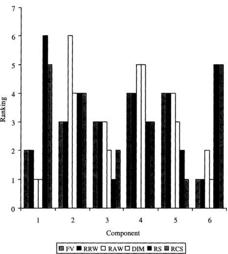
3-9 An example fault tree to illustrate the computation of RS and RCS . 80 3-10 The importance rankings of the components in the example system,

3-11. The importance rankings of the components in the example system, the correlated case ...

3-12 The RRW of the components in the example system in both the

inde-pendent and correlated cases ...

3-13 The RAW of the components in the example system in the both

inde-pendent and correlated cases ...

4-1 The seismic hazard curves of a U.S. nuclear power plant ...

5-1 The probability distributions of the example plant CDF .

5-2 The actual and acceptable uncertainty about the expected

first plant ...

5-3 The actual and acceptable uncertainty about the expected

second plant ... 5-4 5-5 5-6 5-7 6-1 6-2 6-3 6-4 6-5 6-6 6-7

The fault tree of the example system without component 1 RS measures of the components in the example system . . RCS measures of the components in the example system The failure probability distribution of the example system

CDF of the

CDF of the

117 123

...

124

...

126

...

127

...

128

...

131

Block diagram of the CCW system ... Fault tree for the CCW system for the base case .... The simplified fault tree for plant core damage ... FV rankings of the basic events in the CCW System RAW rankings of the basic events in the CCW System RS rankings of the basic events in the CCW System . . RCS rankings of the basic events in the CCW System . . . 135 . . 138 . . 143 . 147 . . 148 . . 149 . . 150

6-8 The fault tree for the CCW System without common cause events . . 152

6-9 Plant CDF unaccounted for due to the omission of common cause events153 6-10 Change in plant CDF unaccounted for due to the omission of common cause events . . . .... 154

6-11 Plant CDF without considering common cause events ... 158

85

86

87 97

6-12 Percentage CDF truncated as a function of truncation limit for the

base case . . . ... 161

6-13 The degree of confidence that the truncated CDF has met the

accep-tance criterion . . . ... 162

A-1 An example fault tree to illustrate the computation of RS for basic events at AND gates by use of the current incomplete model as

refer-ence model . . . ... 174

B-1 The fault tree for the example system to illustrate the selection of truncation limit by use of point estimate approach ... . 179 B-2 The failure probability distribution for the example system without

applying truncation limit. . . . ... 183

B-3 The failure probability distribution for the example system at

trunca-tion level of 1.OE-05 ... 184

B-4 The failure probability distribution for the example system at

trunca-tion level of 2.OE-05 ... 184

B-5 The failure probability distribution for the example system at

trunca-tion level of 1.0E-04 ... 185

B-6 The failure probability distribution for the example system wat

trun-cation level of 5.OE-04 ... 185

C-i Probability distributions of the two non-overlap minimal cut sets ... 188 C-2 Expected fractional truncated risk as a function of truncation limit for

the system consisting of the two example non-overlap minimal cut sets 189 C-3 Probability distributions for the two overlap minimal cut sets ... 191 C-4 Expected fractional truncated risk for the system consisting of the two

List of Tables

3.1 Basic event data for the components in the example system ... 81

3.2 The expected importance measures for the components in the example system, independent case ... 82

3.3 The expected importance measures for the components in the example system, correlated case ... 83

4.1 Contributions to the CDF of the top 20 initiating events for a U.S. nuclear power plant ... 101

4.2 Contributions to the CDF of each operating mode for a U.S. nuclear power plant . . . ... 102

5.1 The distribution characteristics of the CDFs of two example plants 121 5.2 RS and RCS measures for the components in the example system . 126 5.3 The degree of confidence that the RS and RCS of the components in the example system have met the threshold values . ... 129

6.1 Basic events data ... 139

6.2 Model input parameter data ...

140

6.3 Basic events in the simplified plant core damage fault tree ... 140

6.4 Point estimated FV and RAW for the basic events in the base case PRA141 6.5 Point estimated RS and RCS for the basic events in the base case PRA 142 6.6 The expectations of FV and RAW for the basic events in the base case PRA ... 145

6.7 The expectations of RS and RCS for the basic events in the base case

PRA ...

.

146

6.8 Plant CDF and change in plant CDF unaccounted for due to the

omis-sion of common cause events ... 153

6.9 The degree of confidence that RS and RCS of each basic event has met

the threshold values ... 156

6.10 Plant CDF and change in plant CDF unaccounted for due to the

omis-sion of common cause events 14, 17, 18, 19 ... 156

6.11 Uncertainty analysis results for plant CDF without considering

com-mon cause events ... 158

B.1 Means and standard deviations of the component failure probabilities

in the example system ... 182

B.2 The expectation of the percentage truncated system failure probability

at each truncation level ... 183

C.1 Distribution parameters for the two example non-overlap minimal cut

sets ... 188

C.2 Expected fractional truncated risk for the system consisting of the two example non-overlap minimal cut sets as a function of truncation limit 188 C.3 Distribution parameters for the two example overlap minimal cut sets 191 C.4 Expected fractional truncated risk the system consisting of the two

Chapter 1

Overview and Background

1.1 Overview of This Thesis

The final outcome of a Probabilistic Risk Assessment (PRA) is often considered in-accurate and imprecise to some degree. The primary reasons include: certain risk contributors were not considered in the analysis, the analysts may be uncertain about the values of certain input parameters and how the models embedded in the PRA

should be constructed.

In this thesis, we explore methods for assessing the adequacy of PRA results with respect to PRA incompleteness and uncertainty treatment. In particular, we develop measures of risk significance (RS) and risk change significance (RCS), which rank events within a PRA in terms of their importance to the accuracy of the baseline risk and risk change. We investigate the use of RS and RCS to categorize events as either important or unimportant to achieving the desired accuracy level of risk and risk change. We also investigate the use of 9 5th confidence level acceptance guideline for examining the adequacy of uncertainty treatment of a PRA.

This section is followed by a review of the problem of using incomplete and limited scope PRAs for risk-informed decisions. We demonstrate that the adequacy of PRA results required to support an application should be measured with respect to the application supported and the role that PRA results play in the decision making process. We then discuss how the framework developed in this thesis can be used to

assess PRA adequacy.

In Chapter 2 we describe the approach for using PRA results in risk-informed decisions. We first describe existing methods for quantifying logic models such as fault trees and event trees. The methods discussed include qualitative methods for determining minimal cut sets and quantitative methods for computing risk and risk change using the minimal cut sets. We focus particularly on the rare event approxi-mation because it gives fairly accurate results in most cases and it can be computed in less computation time than other approximations. We then describe regulatory guidance for use of PRA analysis in risk-informed activities. The guidance discussed include the U.S. Nuclear Regulatory Commission (NRC) Safety Goal Statement for the baseline risk and the NRC Regulatory Guide (RG) 1.174 on the proposed change in plant design and activities. In the end, three alternative approaches for comparing PRA results with the acceptance guidelines are presented. These approaches include the point estimate value approach, the mean value approach, and the confidence level approach.

In Chapter 3 we develop the concepts of RS and RCS. These measures assess the importance of an event with respect to the impact of its omission from the analysis on the final outcome of a PRA. When the baseline risk is the final outcome of interest, we define the significance of an event as risk significance, measured in terms of the resulting percentage change in the baseline risk. When there is a proposed change in plant design or activities and risk change is the final outcome of interest, we define the significance of an event as risk change significance, measured in terms of the resulting percentage change in risk change. Next, we develop general approaches for computing the numerical values of RS and RCS. These approaches are developed for four groups of events in a logic model: initiating events, basic events whose first operators are AND gates, basic events whose first operators are OR gates, and basic events whose first operators are both AND gates and OR gates. Our significance measures are compared to traditional importance measures such as Fussell-Vesley (FV), Risk Achievement Worth (RAW), and Risk Reduction Worth (RRW) to gauge their effectiveness.

In Chapter 4 we describe three types of epistemic uncertainties in a modern PRA: parameter uncertainty, model uncertainty, and incompleteness uncertainty. We dis-cuss existing approaches for the treatment of each type of uncertainty. We demon-strate that incompleteness uncertainty and model uncertainty can greatly impact both the mean values of PRA results and our confidence in the accuracy of these val-ues. Lack of treatment of these uncertainties is very likely to result in a technically unacceptable PRA.

In Chapter 5 we investigate the use of RS and RCS to identify events that are important to achieving the acceptable degree of accuracy of risk and risk change. We also examine how the 9 5 th percentile acceptance guideline can be used to assess the adequacy of the uncertainty treatment of a PRA. The decision maker's desired degree of accuracy and precision of risk and risk change is typically defined based upon the social consequences of the activity subject to analysis and the role that PRA results play in the decision making process.

Chapter 6 consists of a detailed case study of the component cooling water (CCW) system of a pressurized water nuclear reactor. We first describe the system and the various failure modes considered in our analysis. We then define a base case for computing the RS and RCS for each event in the system. Next, we define a current case where common cause failures of the CCW pumps are omitted from the risk analysis. We then use the framework that we develop to examine the adequacy of the results obtained from the current case PRA in support of a specific applications: the proposed CCW pumps allowed outage time (AOT) extension from 25 hours to 100 hours. Our results suggest that although the FV and RAW importance measures of the common cause failure of pumps 1-1 and 1-3, and the common cause failure of pumps 1-2 and 1-3 during normal operation are relatively low, they are found to be important to achieving the desired degree of accuracy of change in CDF. The PRA model without addressing these two events underestimates the resulting change in CDF by a great amount.

In Chapter 7 we summarize the major contributions of this thesis work and in-dicate how the importance measures we have developed might be used in assessing

the adequacy of PRA results for risk-informed activities. We see how the results ob-tained using RS, RCS, and the 9 5 th confidence level acceptance guideline can indicate which events are important to the accuracy of risk and risk change, and whether the desired accuracy and precision levels have been achieved. It can therefore be useful to decision makers in gauging their confidence level in the risk insights derived from PRA results.

1.2 The Problem of the Adequacy of PRA Results

In this thesis, we focus on the adequacy analysis of PRA results used for risk-informed decisions. The quality of PRAs has been addressed by a number of regulatory and industry organizations [35, 13, 17, 44]. Some have argued that a good PRA should be a complete, full scope, three level PRA, while others have claimed that the quality of a PRA should be measured with respect to the application and decision supported.

In this section, we show by way of an example that the adequacy of a PRA results is important to risk-informed decision making process and should be measured with respect to the application and decision supported. We then discuss several particular decision contexts in which our proposed framework might be useful.

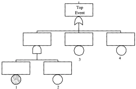
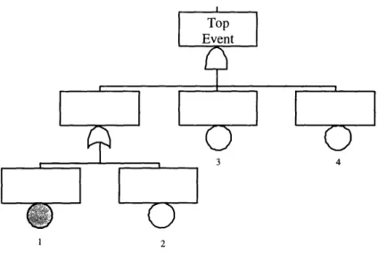
To begin, suppose we have a system consisting of four components. The system configuration is shown in Figure 1-1. Assuming that all component failures probabil-ities are known to the analyst and independent of each other. The failure probability

of each component is given as follows:

PI 1 x 10-3,

P2 = 1 x 10

- 3

_,

p3 =

6 x

10- 3

,

P4 = 8 x 10- 3 . (1.1)

Figure 1-1: A sample system to illustrate the problem of PRA adequacy 4 fails, or components 1 and 2 fail simultaneously. The failure probability of the system can thus be represented as

Qo = P(C

1

C2+C

3

+C

4

)

=

P(ClC

2

) + P(C

3

) + P(C

4

)

- P(C1C2C3) - P(CC2C 4 ) - P(C3C4)

+ P(C1C2C3C4). (1.2)

C(i) is the event that component i fails, and P(Ci) is the probability of the occurrence of event i, or the probability that component i fails. By replacing P(Ci) with qi and truncating the above equation at the linear terms we obtain

Qo qlq₂ + q3+ q4 = 1.4001 x 10-2. (1.3)

Suppose we have two proposed cost-saving changes in the maintenance practice of the components in the system. We would like to know the system failure probability when either of the two proposed changes has been accepted individually. Suppose the two proposed changes in the maintenance practice are:

1. extend the inspection interval of component 2, which results in an increase in the failure probability of component 2 by a factor of four

2. extend the inspection interval of component 3, which results in an increase the failure probability of component 3 by a factor of two

From Equation 1.3, we obtain the system failure probability given that the first proposed change has been accepted as

Q1 - _{qlq2 + q3 + q}

4 = 1.4004 x 10-2. (1.4)

And similarly, the system failure probability given that the second proposed change has been accepted would be

Q2 qlq2 + q3 + q4 = 2.0001 x 10-2. (1.5)

These results indicate that the first proposed change would result in an increase in the system failure probability by 0.021%, while the second proposed change would result in an increase in the system probability by 42.85%.

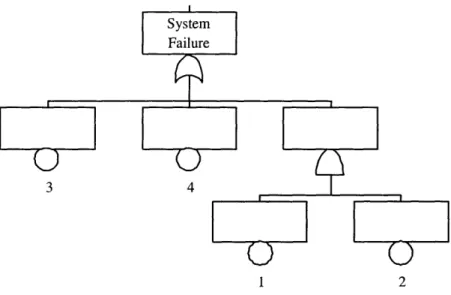
Until now, we have assumed that all causes for the failure of the system have been identified and accounted for in calculating the failure probability of the system. However, certain causal failures may not have been addressed in the risk analysis. This is typically unintentional and results when the existence of these causal failures is not recognized by the analyst due to knowledge constraints, or when their contributions to the system failure is known estimated to be negligible.

In our example, now we suppose the failure of component 1 was not taken into consideration in estimating the failure probability of the system. Under this assump-tion, the potential causes of system failure are: the failure of component 1, failure of component 2, and failure of component 3. In such case, the system failure probability before accepting any proposed changes can therefore be represented as

QO = P(C2+C

3

+C

4

)

P

P(C

2

) + P(C

3

) + P(C

4

)

-

P(C

2

C

3

) - P(C2C

4

) -

P(C

3

C

4

)

+ P(C2C3C4). (1.6)

Again, by replacing P(Ci) with q and truncating the above equation at the linear terms we obtain

(Q - q2+q3 +q4 = 1.5 x 10- 2. (1.7)

The system failure probability after accepting the first proposed change would be

QI - q + q3

+q

4

=

1.8x 10- 2, (1.8)

and the system failure probability after accepting the second proposed change would be

Q2 -- q+q + q4

=

2.1 X 10- 2_{. (1.9)}

These results indicate that, in the case where component 1 is not considered in the model, the first proposed change would result in an increase in the system failure probability by 20.0%, while the second proposed change would result in an increase by 40.0%.

For comparison, the system failure probability for all the six cases is presented in Figure 1-2, Figure 1-3, and Figure 1-4. From these figures we see that the exclusion of component 1 from the analysis results in an overestimate of the baseline system

failure probability by 7.14%, while the system failure probability after accepting the first proposed change is overestimated by 28.54%, and after accepting the second proposed change is overestimated by 4.99%. These numerical values indicate that the simplified model which does not take component 1 into account provides a fairly accurate estimate of the baseline system failure probability and the impact of the second proposed change on the system failure probability. However, its estimate of the impact of the first proposed change on the system failure probability is significantly inaccurate.

Thus, for this particular performance measure, the model which omits the causal failure of component 1 provides adequate information to decision makers who are concerned with the system baseline failure probability and the impact on the system failure probability of the second proposed change. But, it does not provide an accurate risk assessment for decision makers who are interested in knowing the impact of the first proposed change on system reliability.

From this example, we claim that the adequacy of a PRA's results are important for decision makers to make well informed decisions, and that the quality of a PRA should be measured based upon the application and decision supported. A PRA provides adequate information for risk-informed activities in some cases. However, as we have seen in the previous example, in other cases the information derived is inadequate or inaccurate and the PRA model should be improved such that more meaningful information will be obtained and provided to the decision makers for use in risk-informed activities.

.JLJz-UL -1.50E-02 1.48E-02 1.46E-02 1.44E-02 1.42E-02 1.40E-02 1.38E-02 1.36E-02 1.34E-02 Qo Q'

Figure 1-2: System failure probability before accepting any proposed changes

I n"

ZL.UUE-UL 1.80E-02 1.60E-02 1.40E-02 1.20E-02 1.OOE-02 8.00E-03 6.00E-03 4.00E-03 2.00E-03 O.OOE+00 Q1 _Q1'

Figure 1-3: System failure probability after accepting the first proposed change

I frr fi

! I

2.12E-02 2.10E-02 2.08E-02 2.06E-02 2.04E-02 2.02E-02 2.00E-02 1.98E-02 1.96E-02 Q2 Q2'

Figure 1-4: System failure probability after accepting the second proposed change

1.3 Regulatory Approaches for Addressing PRA

Adequacy

Since PRAs can provide useful information to decision makers for managing plant risk and making efficient uses of resources, many nuclear PRAs have been performed throughout the world. In the United States, in order to encourages the use of PRA analysis to improve safety decision makings, the NRC issued a Policy Statement [47] in 1995 stating that

" ...The use of PRA technology should be increased in all regulatory mat-ters to the extent supported by the state-of-the-art in PRA methods and data and in a manner that complements the NRC's deterministic approach and supports the NRC's traditional defense-in-depth philosophy...."

Since then, PRA results have been widely used to measure the risk significance of systems, structures, components(SSCs), to identify the design and operational fea-tures critical to risk, and to identify the events or scenarios leading to system failure. The current activities which involve the use of PRA results in risk-informed regula-tory activities are summarized in a Risk-Informed Regulation Plan issued by the U.S. NRC in 2000 [45] and outlined in the SECY-00-0162 [44]. These activities include: the reactor oversight process for inspection on those activities with the greatest poten-tial impact on safety, operating events assessment for evaluating the risk significance

of operational events, license amendments for providing guidance on risk-informed changes to a plant's licensing basis for inservice testing, inspection, graded qual-ity assurance and technical specifications, risk-informed technical specifications for developing improvements to the technical specifications, and maintenance rules for monitoring the effectiveness of maintenance actions.

PRA, as a quantitative tool, has many strengths as well as weaknesses. There are several limitations on the use of PRA techniques for risk modelling and analysis. First, the true values of most model inputs are unknown. Ideally, probability distribution models are well developed and assigned to the unknown input parameters to reflect

the analyst's state of knowledge of the values of these input parameters. However, due to the analyst's lack of knowledge of where the actual values lie, probability distributions for some parameters can be defined with either overly wide confidence intervals or extremely narrow confidence intervals. The problem of overconfidence and lack of confidence in the values of certain model input parameters can lead to inaccurate PRA results.

Secondly, the analyst's lack of knowledge of a system's practical application as opposed to its theoretical operation can lead to modelling errors. PRAs, like other models. use approximations to make the model manageable and use assumptions to address the uncertainties associated with model structure and input data. When the approximations and assumptions used in developing the PRAs are inappropriate, the PRA results tend to be inaccurate.

Furthermore, most PRAs are incomplete with only a limited scope. Karl N. Fleming [20, 4] pointed out that as many as 20% of events evaluated by the Ac-cident Sequence Precursor (ASP) program including initiating events and acAc-cident sequences are not modelled in existing PRAs. When certain significant component failure modes, initiating events, or plant operating modes are not taken into account in the PRA, both the expectations of PRA results and uncertainties about the ex-pectations are likely to be underestimated.

The difficulty in quantifying common cause failures and human errors also con-tributes to the limitation on the usefulness of PRA techniques. Since common cause failure can cause the failures of several components or systems simultaneously and hu-man action plays an important role in mitigating accidents, they tend to contribute significantly to risk. The inadequate estimates of the common cause failures and human errors can lead inaccurate and imprecise estimate of risk.

Acknowledging these limitations, many nuclear regulatory and industry organiza-tions have established guidance for using PRA analysis in support of nuclear activi-ties. This guidance includes: the American Society of Mechanical Engineers(ASME) standard [35] for probabilistic risk assessment for nuclear power plant applications, SECY-00-0162 [44] on PRA quality in risk-informed activities, NRC Regulatory Guide

DG-1122 [17] on technical adequacy of PRA results for risk-informed activities, NRC Regulatory Guide 1.174 [13] for the use of PRA in risk-informed decisions on changes to the licensing basis, NRC Regulatory Guide 1.175 [14] on risk-informed in-service testing, NRC Regulatory Guide 1.176 [15] on risk-informed graded quality assurance, NRC Regulatory Guide 1.177 [16] on risk-informed technical specifications, and NRC Regulatory Guide 1.178 [18] on risk-informed in-service inspection.

Among the above regulatory guidance and industry programs, the ASME PRA standard identified nine elements which comprise an at-power, internal-events, Level 1 and limited Level 2 PRA. It sets forth the minimal scope and level of detail for PRAs to meet this Standard by specifying a set of requirements for each of the nine PRA elements. Like the ASME standard, SECY-00-0162 addresses the issue of PRA quality by defining the desired scope and technical elements which comprise a PRA model at a function level. The Draft Regulatory Guide DG-1122 defines a technical acceptable PRA by setting forth a set of elements and corresponding characteristics and attributes. We note that, these standards and guidance only define a functional PRA, and they do not ensure confidence in the PRA results.

On the other hand, Regulatory Guide 1.174 states that "... The quality of a PRA

analysis used to support an application is measured in terms of its appropriateness

with respect to scope, level of detail, and technical acceptability. The scope, level of detail, and technical acceptability of the PRA are to be commensurate with the

application

for which it is intended and the role the PRA results play in the integrated

decision process...."

The guidance provided indicates that there is a diverse set of factors influencing PRA quality. However, there appears to be many similarities in these factors. In par-ticular, all guidance recognizes that scope, level of detail, and technical acceptability are key factors in determining the overall adequacy of a PRA. However, they all focus on defining the minimum requirements for a good PRA, and none of them provides an approach for assessing the adequacy of PRA results for specific applications and decisions supported other than in a general sense.

1.4 Applicability of Techniques for Assessing the

Adequacy of PRA Results

In some cases, decisions may focus on ways of improving the completeness of a PRA, for example, by taking into account some of the omitted events in a PRA. Measures of significance, developed in Chapter 3, rank the events in the PRA in terms of the impact of their exclusion from the analysis on the risk level and risk change, and can be a useful tool in this context.

In many other cases, risk-informed decisions focus simply on the acceptability of the estimated risk level, the change in the risk, and perhaps, on the uncertainty about the risk and risk change. In such cases, methods of adequacy analysis of PRA results as those discussed in Chapter 5 can be a valuable tool for the decision making process. In order to be confident in the final decisions on the acceptability of various activities, decision makers may also attempt to reduce the uncertainty level about the risk level and risk change, e.g. by gathering more information about the probability of particular events in the PRA. In such cases, uncertainty importance measures discussed in Chapter 4 can be used to identify which events in the PRA contribute significantly to the overall uncertainty.

There are several limitations on the use of quantitative methods for evaluating the quality of PRAs. This is primarily because results of the evaluation are only as good as the estimates of the model inputs and how accurately the model's structure approximates the actual system subject to analysis.

First of all, the values of certain model inputs may be incorrect because the over-all methodology for treatment of common cause failures and human error is not yet mature. Secondly, most PRAs lack of treatment of dependencies among components, systems, and human actions. In other words, the estimates of the failure probabilities of certain components, systems, and human actions are inadequate given knowledge that other components or systems have failed, or that human errors have occurred.

In addition, the analyst's inadequate understanding of the occurrence of certain initi-ating events or causes to the failure of certain components may result in formuliniti-ating

models that lead to an incorrect estimate of initiating event frequencies and compo-nent failure probabilities.

Another limitation on the use of quantitative methods for evaluating the quality of PRAs is that significant initiating events or component failure modes may be left out of the analysis because their existence was not recognized by the analysts. In such cases, both the PRA results and the evaluation of the adequacy of these results would be incorrect.

Acknowledging these limitations, two important assumptions are made in order to develop our framework for assessing the adequacy of PRA results for risk-informed activities. These two assumptions are:

* Model uncertainty is well treated, and all models embedded in the PRA are technically correct.

* The PRA are fairly complete, and all significant risk contributors are addressed in the analysis.

Despite these limitations and assumptions, the techniques of significance anal-ysis and adequacy analanal-ysis provided in this thesis can provide useful information to decision makers who are concerned with making well-informed decisions on the acceptability of various nuclear activities.

Chapter 2

Existing Approach for Using PRA

in Risk-Informed Decisions

A comprehensive and systematic risk assessment for a nuclear power plant typically consists of deterministic (engineering) analysis and probabilistic analysis. While the deterministic approach provides the analyst with information on how core damage may occur, a PRA estimates the probability of core damage by considering all poten-tial causes. The use of the risk insights derived from PRA results to aid in decision making processes is called risk-informed integrated decision making which is often abbreviated to risk-informed decision making.

The Policy Statement issued by the NRC in 1995[47] states that "...the use of PRA technology should be increased ...in a manner that complements the NRC's deterministic approach and supports the NRC's traditional defense-in-depth philos-ophy." A risk-informed integrated decision making process consists of five elements as described in the RG 1.174[13]. These five elements are shown in the Figure 2-1. Figure 2-2 shows the key elements of a risk-informed, plant-specific decisionmaking process as described in the RG 1.174. From the statement and these figures we note that information derived from the use of PRA methods is only one element of the risk-informed decision making process, and it does not substitute for the results of a traditional engineering evaluation in the decision making process.

in-1.Change meets current regulations unless it is explicitly related to a requested exemption

or rule changes. ,

. Proposed increases in CDF or

risk are small and are consistent with the Commission's Safety Goal Policy Statement.

Figure 2-1: Principles of risk-informed integrated decisionmaking

volves three aspects: the quantification of PRAs, the development of acceptance guidelines, and the comparison of PRA results with acceptance guidelines.

In this chapter, we first describe existing methods for the evaluation of PRA models in general. We then discuss existing regulatory acceptance guidelines for the use of PRA results for risk-informed activities. We also present alternative approaches for comparing PRA results with acceptance guidelines.

2.1 Evaluation of PRAs

The PRA results used to support risk-informed decision making for various nuclear activities typically include: an evaluation of the core damage frequency (CDF) and large early release frequency (LERF), an evaluation of the change in CDF and LERF, an identification and understanding of major contributors to these risk metrics and risk changes, and an understanding of the sources of uncertainty and their impact on the results [44].

Evaluation of PRA models typically involve two different approaches: qualitative evaluation and quantitative evaluation [30]. Qualitative evaluation of PRA models generates minimal cut sets using Boolean algebra analysis for fault trees and event trees. The minimal cut sets are then be used by quantitative methods to produce PRA results and derive risk insights for risk-informed activities.

Several methods exist for both qualitative evaluation and quantitative evaluation of PRA models. In this thesis, we use the rare event approximation as the quan-titative method to evaluate PRAs. The primary advantage of using the rare event approximation is that it is computationally efficient while providing fairly accurate results.

2.1.1

Qualitative Evaluation of Fault Trees

The fundamental elements of a fault tree model are basic events and gates. Basic events refer to component failure and human error which do not need further devel-opment. AND and OR gates are two basic types of logic gates used in the fault tree

model.

The AND gate in a fault tree represents the intersection of input basic events. The gate output occurs only if all of the input events occur. For example, the boolean expression of the output event C of an AND gate with two input events A and B can be written as C = A n B or C = A B. This expression states that, in order for event C to occur, both event A and B must occur. The OR gate, on the other hand, refers to the union of input basic events. The output of an OR gate occurs if one or more of the input events occur.

The top event of a fault tree represents the state of the system of interest, such as the failure of a system to accomplish its function. A cut set of a fault tree is a set of basic events whose simultaneous occurrence leads to the occurrence of the top event. A minimal cut set of a fault tree model is the smallest set of basic events needed to cause the top event to occur. For example, if a fault tree consists of top event C with two basic input events A and B combined by an OR gate, the cut sets are A, B, and AB. The minimal cut sets are A and B. In other words, the occurrence of either event A, or event B, or the simultaneous occurrence of both event A and event B may cause event C to occur. However, in order to cause event C to occur, the occurrence of either event A or event B is sufficient. The simultaneous occurrence of both event A and event B is not necessary to lead to the occurrence of event C.

In order to formulate the minimal cut sets of a fault tree model, we use various rules from Boolean Algebra. The most commonly used rules include:

1 if event i is true xi = (2.1)

10

if event i is false,

l+xi

= 1,

Xi = 1-Xi,

X

= Xi.

(2.2)

For the top event C as discussed above, its Boolean expression can thus be

repre-sented as:

XC = XA + XB (2.3)

For a fault tree with more than one gate, the output of one gate, gate i, is very likely to be the input of another gate, gate j. In this case, the Boolean expression of the output of gate i is then substituted into the Boolean expression of the input of gate j, and so on. This method is the successive substitution method and is the most widely used method in generating minimal cut sets for a fault tree model.

As an example, let's consider the fault tree shown in Figure 2-3. Each node in the fault tree represents an event.

T2 T3 I A A T 4 C T5 1. B B A C B D

Figure 2-3: An example fault tree to illustrate the formulation of minimal cut sets

Starting from the top of the fault tree, the Boolean expression of top event XT is

given as

XT = XT XT2. (2.4)

Where, XT can be written as

XT = XT + XC = XA XB + XC, (2.5)

and XT2 can be written as,

XT2 = XT + XD = XB XT5+ XD. (2.6)

Given

XT5 = XA + XC,

(2.7)

we can substitute XT5 into XT2, and substitute XT1 and XT2 into Equation 2.4 to obtain

XT = (XA XB + XC) (XB (XA + XC) + XD)

= (XA XB +

XC)

(XA

.XB

+

XB.

XC + XD)

XA XB (1 + XC + XD + XC) + XB XC + XC .XD

= XA XB + XB

·

XC + XC ·XD. (2.8)

The final Boolean expression obtained for top event T represents three minimal cut sets with two basic events. The minimal cut sets are events A and B, B and C, and C and D.

As can be seen from this example, it is difficult to determine the minimal cut sets for a large fault tree by hand using the above approach. A number of com-puter algorithms were developed to determine the minimal cut sets for the analysis of fault tree models[40, 39, 49]. In this thesis, we use the SAPHIRE program devel-oped at Idaho National Engineering and Environmental Laboratory (INEEL) which

implements these algorithms to generate minimal cut sets.

2.1.2

Qualitative Evaluation of Event Trees

Unlike the fault tree, which starts with the top event and determines all of the possible ways for this event to occur, the event tree begins with an initiating event and proceeds with the state of each event heading (representing safety system or human action). The occurrence of an event heading i represents the failure of the corresponding system or human action, and the nonoccurrence of event i represents the success of the corresponding system or human action. If the Boolean expression for the occurrence of event heading i is denoted as Xi, the Boolean expression of the success of the event heading i is Xi, or "1 - Xi". However, if an event heading has more functioning states other than success and failure, it would not be possible to represent the event heading using Boolean algebra. In this analysis, we assume that all event headings in an event tree have only two functioning states.

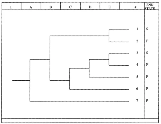
An event tree exhaustively generates all possible combinations of success or failure of all event headings. Any one of such combinations is called an event sequence. Because an event heading either occurs or not occurs at a time, when success and failure of all event headings are combined to generate event sequences, these event sequences are mutually exclusive. The end state of some event sequences is success, while the end states of other sequences is failure. In most cases, only event sequences whose end states are system failure are of great interest to the analysts.

By analogy, the substitution method can also be applied to event trees to generate minimal cut sets. In this case, the cut set of the event sequence with a failed ultimate outcome is the intersection of the failed event headings along the sequence, no matter whether the event heading fails at the beginning of the sequence or at a later time. The overall failure, F, is the union of the cut sets of those event sequences whose end state is failure. If an event heading has its own Boolean expression, its Boolean expression can be substituted into the logic representation of the overall failure F. The reduced Boolean expression of F can then be obtained through the use of Boolean algebra rules.

For example, let's consider the event tree given in Figure 2-4. whose outcome is failure include event sequences 2, 4, 5, 6, and 7. of these sequences are

The event sequences The cut sets of each

Figure 2-4: An example event tree to illustrate the formulation of minimal cut sets

XF

2

= X XE

XF4 = XI XB XE XF5 = XI XB XD

XF

6

= XI XB XC

XF7 = XI. XA. (2.9)

The Boolean expression of the overall failure F, as a union of the above cut sets, is obtained and reduced through the use of Boolean algebra rules as

I A B C D E # END 1 R 2 F 3 S 4 F 5 F 6 F 7 F I

-F

::=

XF

2

+ XF

4

+ XF

5

+ XF

6

+ XF

7

:= XI XE+ XI XB

·

X

+

XXD

X

+

XI

'XB

XC

+

XI XA

=

XI XA +

X

I

XB XC

+

XI XB XD

-

XI XE (1 + XB)

XI XA +

XI

XB XC + XI XB XD + XI XE

(2.10)

The Boolean representation obtained above represents two minimal cut sets with two events, and two minimal cut sets with three events. If event heading XA and XE

are represented by the following Boolean expressions

XA = Xa Xb+Xa

Xc+

Xd

XE = Xa + XbXd+Xe,

(2.11)

then the reduction of the above Boolean expression proceeds as follows:

F =

XIXA+

XI.XB'XC+XI'XB'XD+XI-XE

= XI · (X

a

+ Xd +Xe) + XI 'XB

XC+

XI XB 'XD

= XI Xa + XIXd + XI Xe + XI'XB XC+ XI XB XD

(2.12)

The ultimate minimal cut sets of the event tree are therefore

XiXa, XIXd, XiX, XIXBXC, XIXBXD.

A typical event tree may contain hundreds of event headings. If the number of sequences leading to failure is large, the generation of minimal cut sets by hand using the above procedure is infeasible, especially when event headings contain several additional basic events. However, most PRA software tools are designed to perform

this function, thus the formulation of minimal cut sets for fault trees and event trees can be done easily accomplished.

2.1.3

Quantitative Evaluation of the Logic Models

In the previous section, we discussed how to generate minimal cut sets for fault trees and event trees using the substitution method. In this section, we discuss several methods for quantifying fault trees and event trees based upon the minimal cut sets formulated.

Since the occurrence of a minimal cut set results in the occurrence of the top event of a fault tree, or the failed end state of an event tree, the probability of the occurrence of the top event or failed end state equals to the probability of the union of all its minimal cut sets. For example, if R is the top event or the failed event state of interest, and MCSi is the minimal cut set i (i = 1, 2, ..., n), the exact value of R can therefore be obtained as:

R = p(Z MCSi).

(2.13)

i

The above equation can be expanded as:

R =

Ep(MCSi) i -

p(MCS'

MCSj)

i,j

+

E

p(MCSi MCSj MCSk)

i,j,k (2.14)

The above expression is an exact formulation of R as a function of the probability of each minimal cut set and the probability of the products of the minimal cut sets. When the minimal cut sets are not independent of each other, the evaluation of the cross product terms are difficult. For example, if a basic event appears in several minimal cut sets, then the occurrence of this basic event is likely to cause the

simul-taneous occurrence of all the minimal cut sets, but the likelihood of simulsimul-taneous occurrence of the set of minimal cut sets is difficult to quantify. Thus, when cut sets are dependent, the cross product terms are difficult to evaluate.

If we assume that all minimal cut sets are independent of each other, Equation 2.14 becomes

R =

p(MCSi)

-

E p(MCSi)p(MCSj)

i j>i

+

p(MCi)p(MCj))(MCS3)P(MCSk)

i j>i k>j (2.15)

The above expression is an exact formulation of R as a function of the probability of each minimal cut set. By considering that a minimal cut set often consists of several basic events and/or initiating events, we thus have

p(MCS) = p(U BEi).

(2.16)

m

BEy1 is basic event m in minimal cut set i. If several basic events in a minimal cut set are not independent of each other because of common cause failure or functional dependence, the evaluation of the minimal cut set probability is also a difficult task. Dependencies among the probabilities of basic events can be treated either explic-itly by reflecting them in the structure of the logic trees used to model the system in question, or implicitly by reflecting them in probabilities of basic events and/or initiating events. For example, the failure probability of a system consisting of com-ponents A and component B in parallel is governed by Boolean expression as follows:

Q

= p(AB), (2.17)

Q = p(A) p(BIA) = p(B) p(AIB).

In the above expression, Q is the failure probability of the system, p(A) is the failure probability of component A, and p(B) is the failure probability of component B. p(BIA),p(AIB) is the conditional failure probability of one component given the other component has already failed. If components A and B are functionally or spatially dependent upon each other, the likelihood that one component will fail given that the other component has failed is likely to be higher than independent failure probability. This conditional failure probability must be determined before the system failure probability can be quantified. In the case where the failure probabilities of components A and B are independent of each other, the above equation becomes

Q = p(A) p(B).

(2.19)

Now by assuming that the dependence among basic events is modelled either explicitly in the analysis, Equation 2.15 becomes

R =

(H qI)

i m

-

Ex(1:qm

·

qn)

i j>i m n

+ EE (Iqmq.n Iq)

i j>i k>j m n I (2.20)

The above expression is an exact formulation of R with independent minimal cut sets and independent basic event probabilities. The assumptions of independence result in a much simpler quantitative evaluation of R than the general case shown in Equation 2.14.

We note that, for a PRA model with n minimal cut sets, there are 2-1 cross

product terms, such as (,, qm JIn qj), in the above equation. In order to facilitate the quantitative evaluation of R, some assumptions need to be made. One simplification is to assume that the cross product terms are typically small and can be neglected. The summation of the probability of individual minimal cut sets is thus used as an approximation of the true value of R. Mathematically, we have

R = p(MCSi)=

((

qm).

(2.21)

i i m

We note that, this approximation of R yields an upper bound on the true value of R, therefore it is denoted as the upper bound approximation of R. Since the cross product terms are truncated for their low probabilities of occurrence, this approxi-mation is also called the rare event approxiapproxi-mation.

By analogy, we can obtain the lower bound on the true value of R by keeping the cross product terms containing two minimal cut sets, and neglecting the ones containing three or more minimal cut sets as follows:

R =

Zp(MCSi)

-

Z

p(MCSi) p(MCSj)

i i j>i

(I

q)

)-

ET

(

q'

I q)

(2.22)

i m i j>i m n

In general, the lower bound approximation tends to be more accurate than the rare event approximation. However, the rare event approximation is much simpler in the physical form and easier to compute than the lower bound approximation. Further-more, the rare event approximation gives fairly accurate results for most applications. Therefore, the rare event approximation is used throughout this thesis.

Although initiating events or basic events may appear in many different minimal cut sets, they generally appear at most once in each minimal cut set[51, 53]. The rare event approximation can thus be generalized with respect to a specific initiating event or basic event as:

R = ai · qi + bi.

(2.23)

Where qi is initiating event frequency or basic event probability. ai qi is the sum of all the minimal cut sets that contain event i, and bi is sum of all other minimal cut sets that do not contain event i.

The above expression is the most widely used formulation of R with respect to ba-sic event probabilities. It is derived from the rare event approximation and under the assumption of exclusive independence among basic event probabilities. By analogy, the formulation of R with respect to any two events can be obtained as [51]:

R = aijqiqj aiqi + ajqj + bj.

(2.24)

Where,

* aijqiqj represents all of the minimal cut sets which contain both events i and j * aiqi represents all of the minimal cut sets which contain event i but not j * ajqj represents all of the minimal cut sets which contain event j but not i, and * bij represents all of the minimal cut sets which contain neither events j nor i By analogy, we can obtain the formulation of R as a function of any three events in the PRA, any four events in the PRA, and so on. However, when the number of events involved increases, the formulation of R becomes rapidly more complex and is of little use in practice.

2.2

Quantitative Evaluation of Risk Changes

In the previous section, we present two commonly used approximations for the risk metric R. In this section, we discuss the quantitative evaluation of risk changes based upon the rare event approximation and the assumption that all event probabilities are mutually independent.

By taking the derivative of Equation 2.14 with respect to qi and rearranging the terms we obtain

OR ai qi qi (2.25)

R

R

qi

This expression is a general formulation of the resulting change in risk that could result from an infinitesimal change in probability of event i. This relationship can also apply to a finite change in the probability of event i. In this case, the resulting change in the overall risk level is

AR ai qi Aq (2.26)

R

R

qi

This above equation indicates that the change in R is proportional to the change in the event probability.

However, in most cases, a proposed change in the plant design or activities is likely to affect a set of basic events. According to Equation 2.24, when both basic events i and j are affected by an activity simultaneously, the resulting change in R is governed by

AR,,j = aij(AqiAqj + qiAqj + qjAqi) + ajAq + ajAqj.

(2.27)

By rearranging the terms in the above expression we can show that

ARi,j = (aijqj + ai)Aqi + (aijqi + aj)Aqj + aijAqiAqj

= ARi + AR, + aijAqiAqj.

(2.28)

where AR is change in risk that could result from a Aqi change in the probability of basic event i while all other event probabilities are fixed at their nominal values. ARj is risk change due to a Aqj change in the probability of basic event

j

while keeping all other event probabilities unchanged. By dividing both sides by the baseline risk,

R, we have

ARij aiqi Aqi ajqj Aqj aijqiqj Aq, Aqj

- - (2.29)

R R qi R qj R qi qj

We note that the first two terms are percentage changes in risk that could result from changes made to basic event i and j one at a time. The third term represents the additional risk change due to simultaneous changes in both basic event probabilities. If an activity under consideration affects more than two basic events, Equation 2.29 can be generalized as AR aiqi Aqi

R

R qi

E E aijqiqj Aqi Aq i j>i R qi qj + aij...nqjqj q'q Aq Aqj q... (230) qi qj j

Under some circumstances, e.g. the change in the probabilities of basic events are small, the cross term is small enough to be dropped. In such cases, the above equation reduces to

AR = aiq Aqj (2.31)

R E· R qi

Unfortunately, there will be situations where the cross terms are not negligible. In these cases, knowing only the risk change of individual basic events from Equation 2.26 does not provide enough information to compute the risk change that could result from changes in the probabilities of a group of basic events. To overcome this problem, a so called risk/safety monitor program[26, 32, 23] has been developed. A risk monitor is a software algorithm that can quickly reevaluate the PRA model when one or more changes are made, especially during maintenance activities.