Controlling fuel and diluent gas flow for a diesel engine operating in the fuel rich low-temperature-combustion mode

(1)

Controlling Fuel and Diluent Gas Flow for a Diesel Engine Operating in the Fuel Rich Low-Temperature-Combustion Mode.

by

David M. Lopez

Submitted to the Department of Mechanical Engineering in Partial Fulfillment of the Requirements for the Degree of

Bachelor of Science in Mechanical Engineering at the

Massachusetts Institute of Technology June 2007

The author hereby grants to MIT permission to reproduce and to distribute publicly paper and electronic copies of this thesis document in whole or in part in any medium now known or

hereafter created.

Signature of Author:

Department of Mechanical Engineering May 1 l, _{2 0 0 7}

Certified by:

Wrai K. Cheng Professor of Mechanical Engineering

'S"nimm, LThesis Supervisor

Accepted by: MASSAC-HUSETTS INS E OF TECHNOLOGY

EJUN

212007AAR

L~ARIES

John H. Lienhard V Professor of Mechanical Engineering Chairman, Undergraduate Thesis Committee

~v · rr r·· ·

IF

(2)

(3)

Controlling Fuel and Diluent Gas Flow for a Diesel Engine Operating in the Fuel Rich Low-Temperature-Combustion Mode.

by David M. Lopez

Submitted to the Department of Mechanical Engineering on May 11th, 2007 in Partial Fulfillment of the

Requirements for the Degree of Bachelor of Science in Mechanical Engineering

Abstract

The flow of a diluent gas supplied to a motoring engine was controlled at a diluent to air mass flow ratios of 10%, 30%, 50%, and 70%. This arrangement was a significant set up for running the engine in the Low-Temperature Combustion mode. The engine used was a 436 cc Yanmar Diesel engine, driven at constant 2200 rpm by a 10 hp AC powered dynamometer. Intake air flow was measured by a model FMA-903-V Air Velocity Transducer by Omega Engineering, Inc., and the diluent gas flow was both measured and controlled by a model FMA-2613A Mass Flow Controller, also by Omega Engineering, Inc. Both were connected to a computer through a National Instruments USB-6211 data acquisition hub, and the signals from both were processed in real time through National Instruments' LabView 8.2 software. The

diluent gas used was nitrogen.

The flow controller was found to have reasonable flow precision but poor flow accuracy at many of the flow rates encountered during this experiment, with a minimum steady state error of 3.7% for a flow rate of 207.4 Standard Liters Per Minute (SLPM), the highest flow studied, and a maximum error of 97.4% at 53.8 SLPM, the lowest flow studied. The substantial error at low flow rates stems from the rated lower flow limit of the controller of 250 SLPM. A relation describing the amount of steady state error present was determined empirically, and either this equation or the implementation of an external PI controller can be used in the controlling LabView environment to decrease the steady state error.

Thesis Supervisor: Wai K. Cheng

(4)

(5)

Acknowledgments

I would like to thank Professor Wai K. Cheng for agreeing to advise me on my thesis

project. His patient guidance throughout the last few months while I have been working on this project was a great help to me.

I would also like to thank the students and researchers of the Sloan Automotive

Laboratory. They were extremely helpful and informative when I had questions about the programs and experimental setup that I was using, and really helped make this project go much

more smoothly than it otherwise would have.

I owe my greatest thanks to my family and friends for helping me pull everything

together over the last few years, especially my girlfriend, Stephanie, and my parents, Pablo and Denise. Without their guidance and support throughout my life, I would not be here. Much of what I am, I owe to them.

(6)

1.3: SCOPE ... 11 CH APTER 2 ... 12 2.1: EQUIPMENT... ... ... ... 12 2.1.1: Engine/Intake... ... ... ... ... 12 2.1.2: Dynamom eter... ... ... 12 2.1.3: Airflow Sensor ... ... ... 13 2.1.4: Flow Controller .... ... ... ... ... 13 2.1.5: D iluent Gas... ... ... 14 2.1.6: D ata Acquisition ... ... ... . ... ... 15 2.2: EXPERIMENTAL SETUP... ... 19 2.2.1: Physical Setup... ... ... ... ... ... 19 2.2.2: Software Setup ... .... ... 20 2.3: EXPERIMENTAL M ETHODS... ... 21 2.3.1: Engine M otoring... ... ... ... 21

2.3.2: Controller Step Response... ... 21

2.3.3: D iluent Gas Flow Control ... ... ... ... 22

2.3.4: D ata Collection... 22

CH APTER 3 ... 23

3.1: ENGINE SPEED VS. CLUTCH COIL CURRENT ... ... 23

3.2: FLOW CONTROLLER STEP RESPONSE ... ... 24

3.3: FEEDBACK FLOW CONTROL ... 27

CH APTER 4... 33

4.1: SUMMARY ... 33

4.2: FUTURE W ORK ... 35

REFEREN CES ... ... . ... 37

APPENDIX A : ENG INE SPEED VS. CURRENT ... ... 38

(7)

List of Symbols and Values

Symbol Air Properties* [4] [air Pair Nitrogen Properties* [ [LN2 PN2

Intake Pipe Propertie:

d A Tubing Properties. dtube Name Dynamic Viscosity Density Dynamic Viscosity Density Inner Diameter Cross Sectional Area

Inner Diameter Value 18.4332x10-6 _{kg m}1 _s-1 1.1839 kg m-3 17.7820x10 -6 _{kg m}1 _s1 1.145 kg m3 0.05318 m 0.0022 m2 0.0254 m

*Gas Properties taken at 250C, 14.695 PSIA +Measured/Calculated Value

(8)

Chapter 1 Introduction

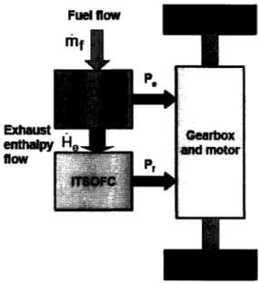
The purpose of this study is to examine the feasibility of a diesel and fuel cell hybrid powertrain for long haul transportation as well as establishing an initial baseline control scheme for the system. The proposed configuration involves the combination of an Intermediate Temperature Solid Oxide Fuel Cell (ITSOFC) with an Internal Combustion Engine (ICE)'. The ICE will run in the fuel rich Low-Temperature-Combustion (LTC) mode to increase hydrocarbon (HC), carbon monoxide (CO), and hydrogen (H₂) emissions of the engine, which the fuel cell can then use to generate power. [1] Fuel flow Exhausl enthalpi flow Gearbox and motor

Figure 1: Proposed Hybrid Powertrain Schematic. Reprinted with permission from

Cheng and Hahn. [3]

In order to run this assessment study, an experimental setup in which the air-fuel ratio and residual gas fraction can be controlled so as to examine the effects of these variables on overall system performance.

(9)

1.1: Importance

The proposed hybrid powertrain can significantly raise the overall thermodynamic efficiency over that of a simple IC engine. Losses in the IC engine itself are decreased due to the lower combustion temperature of an engine running fuel rich. The ITSOFC can convert the chemical energy remaining in the exhaust stream with a conversion efficiency of 45% to 65%, which represents an 8 to 32 percentage point increase over that of a conventional IC engine. This added conversion efficiency results in the use of a greater proportion of the chemical availability of the fuel being consumed, thus decreasing fuel consumption for a given output. [1]

The use of the onboard diesel engine as a fuel reformer offers further efficiency benefits over conventional reforming processes. Traditionally, the waste heat generated through the reformation of petroleum based fuels into the H2 and CO that a fuel cell uses

to make power is largely wasted. This unutilized heat represents both an efficiency penalty and a size and weight penalty, since the processed steam usually requires further processing to cool it before its exhaustion. These penalties are especially concerningin the eyes of the transportation industry, where fuel consumption, size, and weight are of paramount importance. The use of the diesel ICE as both a power generator and fuel reformer largely avoids these problems, however, and registers substantial increase in the overall fuel conversion efficiency of the complete system. [1]

Besides this efficiency benefit, the combination of a diesel engine and a fuel cell offers several other advantages over a fuel cell only powered vehicle. The chemical reactions that take place in a fuel cell will not occur below a certain operating temperature, the exact value of which depends on the structure and materials used in the fuel cell. Normally, a fuel cell must be heated via an external source when the vehicle is first "started" before it will begin producing electricity. This means that the vehicle operator must have a source of heat and also must wait until the fuel cell has warmed to operating temperature before the vehicle is fully functional. With this hybrid setup, the warm exhaust gases of the diesel engine can be used to heat the fuel cell, and the vehicle will run as on a standard diesel engine until the fuel cell is ready for operation. [1]

(10)

1.2: Overview of Prior Research

Previously, some research has been done on lower compression ratio (CR) engines to examine their fuel rich characteristics up to a fuel equivalence ratio (0, defined as the actual fuel/air ratio over the stoichiometric fuel/air ratio, so that D > 1 denotes fuel rich operation) of 1.2. The engine used in this experiment was a Mazda 2.3L 14, which shares its base architecture with the 2.3L engine found in the Ford Ranger. Only one cylinder was fired, and the other three cylinders were simply motored during test runs. Compression ratio was raised from 9.7:1 to 11:1, customized camshafts were ground for shorter duration, and exhaust cam timing was advanced up to 35 crank angle degrees (CAD) from its initial position to control the residual gas fraction.

S.8 loe

c

0.4

s

i 1.5 2 2.5 3

Fuel equivalence ratio (0)

Figure 2: Exhaust Chemical Energy vs. Fuel Equivalence Ratio. The blue line is theory, data points are from the 2.3L Mazda 4 cylinder. Reprinted with permission from Cheng

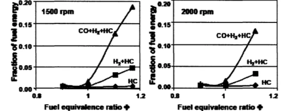
and Hahn. [3] p0,20" _D2O _{1500 rpm} 10,20 e0.15 0 0..05 0 6.10 •"'nn c..000 0s 1 1.2 0. 1 1.2

Fuel equivalence ratio 4 Fuel equivalence ratio +

Figure 3: Exhaust Chemical Energy, data points from the 2.3L Mazda 4 cylinder engine. Reprinted with permission from Cheng and Hahn. [3]

I Soot production

A

1500 rpm data

A 2000 rpm data

(11)

The results of this experiment show that the chemical availability of the exhaust increases rapidly as the air-fuel ratio richens. This shows that the idea of an ICE-ITSOFC hybrid has merit for a low compression ratio spark ignition engine. However, studies still must be done to prove that a higher compression ratio, compression ignition engine can operate in the same mode and shows the same promise.

1.3: Scope

In order to assess the operation and performance of the diesel-ITSOFC hybrid

powerplant configuration for a long haul trucking application, the analysis of a diesel engine operating in LTC mode as a fuel reformer is required. To ensure timely and economical assessment, a small single cylinder diesel engine was used for preliminary assessment. Due to the low volatility of diesel fuel, the engine's current injection hardware is insufficient to ensure adequate fuel-air mixing for the fuel-rich LTC mode under examination. Propane will stand in for diesel fuel during the initial assessment. A mixture of CO2, N2, H2, and CO will be supplied to the intake stream to simulate the

significant EGR required to prevent significant knocking. Thus, the experiment will involve the control of fuel and diluent flow into a single cylinder diesel engine. [2]

The main goal of this experiment is the implementation of fuel and diluent gas flow control. The hardware needed to run this experiment will be set up, which includes the engine plumbing, sensors, flow control actuators, and the interface between the sensors and actuators and the computer. A feedback control program will be engineered using National Instruments' LabVIEW 8.2. Initially, only diluent flow will be controlled, but the LabVIEW program will be set up to allow easy expansion so control of the fuel flow can be implemented at a later date using the existing program. To obtain air flow numbers and verify the operation of the controller at steady state, the engine will be motored at constant engine speed by an attached dynamometer.

(12)

Chapter 2 Experimental Information

2.1: Equipment

2.1.1: Engine/Intake

The engine used in this experiment is a four-stroke single-cylinder Yanmar L100V direct-injection naturally aspirated diesel engine. This engine has a bore of 86 mm and a stroke of 75 mm, for a total cylinder displacement of 436 cc. It has a compression ratio of 19.5:1, sufficiently high to ensure fuel combustion. Its maximum operating speed is 3600 rpm, but for the purposes of this experiment it will be run at approximately 2200 rpm.

There are two large tanks in its intake path between the air flow sensor and the engine itself. These tanks act to dampen the cyclic surge of air into the cylinder during the intake process, allowing the air sensor to see an average unidirectional flow rather than a rapidly fluctuating flow. This average flow reading will be of greater use as an input signal to the flow controller that meters the diluent gas flow, since this controller will then only be called upon to hold an average flow value rather than releasing gas in short, high flow rate bursts.

The fuel pump of this engine is contained within the block itself and so is quite difficult to access and disable. This pump uses fuel to cool itself, so to ensure that it would not fail and adversely affect engine performance during testing, a small amount of diesel fuel is added to the engine's fuel tank. Since no diesel fuel is needed to run the engine for this experiment, the fuel pump's output line is connected directly to the fuel return on the fuel tank.

2.1.2: Dynamometer

The dynamometer used to motor the engine was a 10 horsepower, 3500 rpm motor made by The Louis Allis Co. This dynamometer is coupled to the engine via an electromagnetic clutch. The clutch lockup, and thus torque transfer, is controlled by current that is sent through the clutch. The more current that is passed through the clutch,

(13)

the more torque is transmitted through it, so the faster the engine will spin. The current is controlled by setting the voltage across the clutch via a BK Precision 1670A DC Regulated Power Supply, operating between 0 and 30 Volts. The engine was run at 21 Volts. More information on engine speed versus power supply voltage can be found in

Appendix A.

2.1.3: Airflow Sensor

The Airflow sensor used was a FMA-903-V Air Velocity Transducer by Omega Engineering, Inc. This sensor measures standard velocity, so called because it references the mass velocity of air to standard conditions, 250_{C and 760 mm Hg. This allows for}

measurements that do not require pressure or temperature correction. This particular sensor measures a corrected velocity of zero to 1000 standard feet per minute (SFPM) of

flow, which is output as a reading of zero to five Volts. To convert this SFPM of flow to

a more useful mass flow, the following relation may be used:

1000 SFPM

mhir =•V* SFPM *1000 * Pair (1)

5 Volts

where V is the output voltage of the sensor, 1000/5 is the conversion factor between sensor voltage and SFPM, A is the area of the duct, and Pair is the density of air at standard conditions. [4]

2.1.4: Flow Controller

The flow controller used was also from Omega Engineering, Inc. It was a

FMA-2613A Mass Flow Controller, rated to control and measure mass flows from 250+ to 1000 standard liters per minutes (SLPM) [5]. An input signal from zero to five VDC sets

the desired flow set point, a voltage of zero corresponding to zero flow and one of five corresponding to the maximum flow supported by the controller. The flow controller also provides a flow reading, from zero to five VDC, of the actual flow through the device. The set point and flow readings, both in SLPM, vary linearly with voltage. To ensure that this was the case, voltages were supplied to the controller and the resulting set points recorded. The results can be found in Table 5 in Appendix B. To convert SLPM values into mass flows (in [<mass>/min]), simply multiply the SLPM reading by the density (in [<mass>/L]) of the gas being metered [5].

(14)

It contains an internal controller with programmable proportional (P) and derivative (D) gain constants. Altering the proportional gain alters the speed at which the controller responds to a new input, and altering the derivative gain alters the damping constant of the system, decreasing overshoot and settling time. For this experiment, the constants were set to P = 600 and D = 16000, slightly altered from the factory settings of P = 200 and D = 16000. These values were found to provide adequate controller response for the control of the diluent gas flow. See Section 3.2 for more discussion on controller response.

This flow controller has the ability to control flows of several different gases from the factory, and provides a menu to select one of these gases to let it know which it is dealing with. However, it can also control other gases not on the factory list, though a few corrections must be applied. The given the flow rate indicated by the flow sensor and the dynamic (or absolute) viscosities of both the selected gas and the alternate gas. The flow rate of the alternate gas, Qait, can then be found:

a1t = given s (2)

where Qgiven is the flow rate given by the controller, psel is the viscosity of the original, selected gas, and Msel is the viscosity of the alternate gas being passed through the fuel

controller. [5]

This experiment requires control of nitrogen gas flow, which is supported by the controller from the factory and so does not require the use of Eq. (2). However, if nitrogen is replaced by a mixture of other gases to more closely simulate residual gas properties, Eq. (2) will be quite helpful. Viscosities of the gases used have been provided in the section List of Symbols and Values above for future reference.

2.1.5: Diluent Gas

The diluent gas used in this experiment is nitrogen. A pressurized tank of nitrogen gas provides a source of the gas, and its pressure regulated via an Airco pressure regulator so that the gas enters the flow controller at 40 psi. This provides adequate pressure to reach the flow rates required to hold the mass flow of the diluent gas at approximately 70% that of the air flow entering the engine, which is the richest data point required.

(15)

2.1.6: Data Acquisition

The interface between the computer and the external sensors and controller is a National Instruments USB 6211 hub. This hub has several analog input and output ports through which the sensors and the N2 flow controller are connected, respectively. There

are enough input and output ports to support expansions when fuel flow control is desired.

To collect and process the data, National Instruments' LabView 8.2 was used. The front panel view and block diagram of the program, called a virtual instrument (VI), are shown below in Figures 3 and 4, respectively.

Figure 3: LabView Front Panel View.

The front panel contains all of the user inputs and visual outputs of the LabView virtual instrument. The three graphs dominate the screen. The leftmost display charts the incoming voltage of the flow controller and the upper right chart displays the flow sensor input voltage. The bottom graph shows the output voltage sent to the flow controller to give it its set point. In the bottom left corner are other readouts and user controls. One

(16)

input box allow the user to set the N2 flow as a percentage of the incoming air flow, and

the other allows a constant voltage offset to be added to the system, useful for testing the flow controller response to step inputs after controller constants are altered. There are also two readouts that give both air flow and N2 flow in units of kg/min. There is a

toggle switch that allows the VI to ignore the input from the air sensor, so N2 flow can be

controlled solely by the offset voltage input. Finally, there is a stop button that halts the operation of the VI. The upper right corner has a file input box that lets the user input a file path and name for the recorded measurement file written by the VI, a file path indicator box that tells the user where the file has been recorded, and a LED that signals whether or not the incoming data is being saved.

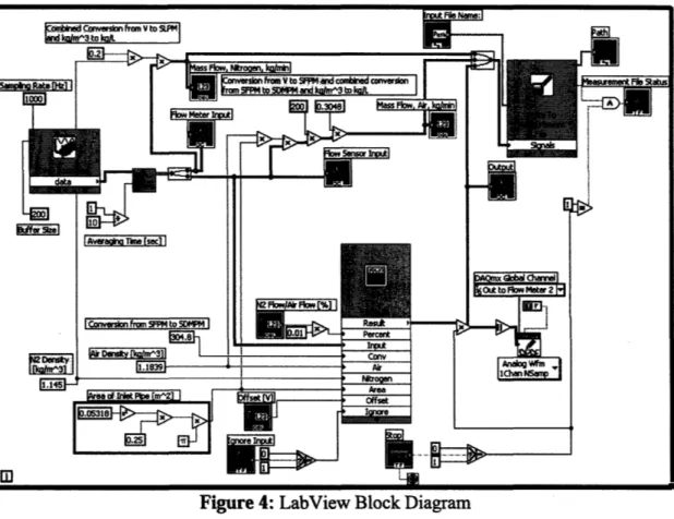
Figure 4: LabView Block Diagram

The LabView block diagram is the part of the program that takes the inputs given to it through the front panel and data acquisition equipment and runs these values through calculations to return the desired output. The voltage input signals from the USB are read at a rate of 1000 samples per second and then fed to an averaging block. This block averages 0.10 seconds, or 100 points, worth of data to create a single value 10 times

(17)

every second for each incoming signal. These averaged signals are then split so that they can be analyzed and manipulated separately. There are two signals in this case, one for the air flow and one for the diluent gas flow, both raw voltages at this point. The voltage of the air flow then enters the formula block, where it is then operated on by the following equation to transform it to the voltage required by the flow controller to allow the correct N2 flOW:

JUr ] V34 L *lSFPM *A[m2]*Pr* o ffset (3) Vou, = x[%]* V,,[V]* 304.8 - SFPM* A[mN2 Pair * Igore +Voe (3)

m2ft

SLPM

PN,2

In the above relation, x is the desired percentage of the air mass flow, Vi, is the incoming voltage from the air flow sensor, and the constant 304.8 is the conversion from feet to meters (1 ft = 0.3048 m) and from liters to cubic meters (1000 L = 1 m3

). The

next term, 1, is the conversion from the voltage input by one SFPM to the voltage input by one SLPM. Since each device operates on a scale of 0-5 V, where zero refers to zero SFPM/SLPM and five refers to 1000 SFPM/SLPM, a given voltage refers to the same numerical value of standard mass flow for either sensor, though the units differ. The term A refers to the area of the intake pipe, and the two ps refer to the densities of air and nitrogen, given by the subscripts in the equation. The voltage V,,out will then tell the controller the SLPM needed to flow mN2 = x*mair _{of nitrogen gas. The last two terms,} Ignore and Voffest, cause Vout to deviate from the value needed to fulfill the above

requirement. Ignore is either one or zero, depending on the position of the toggle switch on the front panel, so it either allows Vin to affect Vout, or it tells the formula to ignore the air mass flow when determining the nitrogen mass flow. The final term, Voffset, allows the formula result to be offset by a constant number. If the toggle switch on the front panel is flipped on, Ignore is set to zero, thus negating the effect of Vi, and so Vou, = Voffset.

When the stop button is pressed, several things must happen for the system operations to truly come to a halt. The output voltage sent to the flow controller is set to zero so that the valve closes and theoretically ceases to flow gas. This is important, because the USB hub will continue to output its last set voltage after the VI ceases to provide new inputs, so the flow controller would be set at its last known flow rate even after the experiment has stopped. This would waste gas and, in the case of fuel control, would cause a potentially hazardous situation if the engine were to be halted or its

(18)

operating speed changed via the dynamometer while fuel was still flowing. The measurement file status indicator LED is reset so that it reports no data being written while the VI is off. This LED also holds its last known value when the VI is halted unless otherwise specified, so it will report that data is being written even when the VI is non-operational if it is not told to display otherwise when the stop button is pressed. Finally, pressing the stop button breaks the loop that the VI operates in, stopping its

operation.

To add a fuel controller, only a few changes must happen. The VI can be modified by adding one more input to the DAQ Assistant that handles the inputs and one more output block, as well as a new formula block to set the new A/F ratio. Alternatively, a new DAQ Assistant could be added to handle both outputs, if LabView gives trouble with two separate output blocks. An input for equivalence ratio should be added to the front panel of the VI so that it can be easily changed by the user. The new formula would closely resemble Eq. (4), assuming a similar flow controller is used for fuel control:

F L SFPM P

Vu = ** V• [V] * 304.8

*1

* A[m2 ]* Pair Ignore + V (4)

ou A m2ft SLPM Pe ofse

where D is the equivalence ratio and F/A is the stoichiometric fuel-air ratio for this fuel. This equation assumes that the flow controller supports the fuel used. If this is not the case, then Eq. (4) can be used to compensate for the readings of the new gas.

(19)

2.2: Experimental Setup

2.2.1: Physical Setup

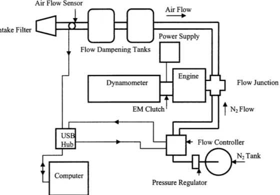
Air Flow Sensor

Intake Filter

Junction

Figure 5: Block Diagram of the Experimental Setup.

The intake filter is attached to the end of the 53.18 mm diameter intake tube. The air flow sensor measures the flow in a straight tubing section with a well defined cross-sectional area, between the intake filter and the first flow dampening tank. Next in the intake path are two large tanks connected in series. These tanks are meant to dampen out the rapid fluctuations in flow that occur when the intake valve opens and closes, allowing air to quickly flow for short periods of time. These variations would be very hard for the air flow sensor to measure accurately and so could introduce significant error into the average flow value obtained by the air flow sensor, so readings should be much improved if flow variations are dampened out.

After the dampening tanks, the intake air flows through a 1 inch inner diameter tube into a three-way flow junction. One end of the junction is for the air, one is for the fuel, and the last is for the diluent gas. The fuel connection is blocked off for the time

(20)

being, since fuel is not being introduced into the system. After air enters this junction, it enters the cylinder, and then is expelled through the exhaust.

The nitrogen's path is similar to that of the air. The gas was supplied by bottled gas through a pressure regulator. It then flows through a 0.25 inch inner diameter tube into the flow controller. From the output port of the flow controller, the nitrogen flows through a 1 inch inner diameter tube into the three-way connector. From there, it enters the cylinder and is then expelled through the exhaust.

The engine itself is coupled to a dynamometer via an electromagnetic clutch. There is a power supply that regulates the current running to the clutch, controlling clutch lockup and, thus, engine speed. This allows the engine to be motored, so air flow measurements can be taken and diluent flow control can be examined without actually burning fuel and dealing with the results of combustion.

All sensor inputs go to the analog input ports on the National Instruments USB hub, and all control outputs originate from this device. As currently set up, the air flow sensor is plugged into channel ail, and the flow controller's flow sensor is plugged into channel ai0. The output to the flow controller comes from channel aol. The specific channels are not overly important, however, because they can easily be changed in LabView. As long as all inputs are plugged into analog input ports and all outputs are plugged into analog output ports, then the rest can be taken care of in the software, requiring at most the swapping of some wires in the VI block diagram.

2.2.2: Software Setup

The software is largely set up for plug and play use. Once the input and output channels are configured, little editing is required to get the experiment to run smoothly on the software side. Sampling rate and buffer size can be changed, but care must be taken to keep a sampling rate and buffer size in the correct proportions so that errors do not crop up when LabView goes to read data that has already been overwritten or is not yet there. It seems that a buffer size of one-tenth to one-fifth of the sampling rate is ideal and prevents any of these errors from occurring.

(21)

2.3: Experimental Methods

The purpose of this experiment is to measure the steady state performance of a feedback flow controller that regulates the mass flow of a gas at a rate equal to a certain percentage, by mass, of that of the intake air. For now, this gas is simply diluent gas, though these experimental methods are identical if fuel flow were to be measured.

2.3.1: Engine Motoring

During this experiment, the engine must be run to provide air flow values for the air flow sensor to pick up and feed to the LabView VI so that the flow controller has realistic inputs to work with. Since fuel will not be provided to the engine, it cannot power itself, so the dynamometer is used to motor the engine. It is the steady state performance that is to be examined, so the dynamometer is run at steady state. To ensure that the engine has reached its steady state operating speed, the equipment is allowed to run for a period of two minutes after the power supply has been set to the desired level before flow testing starts.

For the determination of engine speed as a function of clutch current, the power supply is used to output a desired current by adjusting the voltage. The optical tachometer is then used to measure engine speed. Once the engine speed ceases to rise or fall and begins to oscillate slightly around a constant value, it is recorded and a new current is set to continue the cycle and produce another data point.

2.3.2: Controller Step Response

The controller step response was obtained by giving the controller a zero to one volt step command. This was done using the VI software. The "Ignore Input" toggle on the front panel was flipped on, thus ignoring input from the air flow sensor. The VI was started and allowed to run for a short time to ensure that a steady state condition had been reached. Then, the offset voltage was changed from 0 V to 1 V, resulting in a similar change sent to the controller. The controller then responded to the resulting step jump in set point, and data was collected and analyzed for 10%-90% rise time, 5% settling time, the percent overshoot, and steady state error.

(22)

2.3.3: Diluent Gas Flow Control

The tank of pressurized nitrogen gas is connected to the pressure regulator and the pressure seen by the flow controller is set to 40 psi. This pressure was found to be adequate pressure to allow enough nitrogen flow that all required N2/air ratios could be

examined. The engine is brought to steady state as described in Section 2.3.1, and then the VI was started. The program immediately begins sending set point information to the flow controller, and after approximately five seconds of operation this set point signal

settles to its approximate steady state value.

2.3.4: Data Collection

Data collection is managed by the LabView VI. The user inputs a file path and name through the text box on the front panel view of the VI, and a LabView measurement file (*.lvm) is written there, continually updated as more samples are taken and signals sent out. The text file consists of a header, which contains data about the version numbers of the LabView reader and writer, the date and time data is taken, and any descriptive comments written into the file. The bulk of the output measurement file is written in four tab-delimited columns, the first being time, and, with the current setup, the second is the mass flow of nitrogen, the third the mass flow of air through the intake, and the fourth consisting of the output set point voltages. This data is written in simple text format and so can be imported to a variety of data analysis programs, including, but not limited to, Microsoft Excel, Matlab, and Mathsoft Apps' MathCAD. This is all done automatically with no input past a file name required of the user. If the file cannot be found after creation, check the output dialog box labeled "File Path" beneath the file path and name input box. The path and name of the last file written will be displayed here until the VI is started again.

(23)

Chapter 3 Results and Discussion

3.1: Engine Speed vs. Clutch Coil Current

As mentioned previously, the engine speed is controlled by the current flowing through the electromagnetic clutch that connects the engine to the dynamometer. It should follow that a map of the engine speed as a function of clutch current could then be made, allowing for easy prediction and control of engine speed using the power supply.

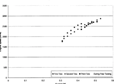
Engine Speed vs. Clutch Current 3500 3000-2500 B 2000 . 15oo00 1000 500 0 0 _ 0 *E

OFistTest e Second Test UIThirdTest During Flow Testing

0 0.1 0.2 0.3 0.4 0.5 0.6

Current JAI

Figure 6: Engine Speed vs. Clutch Coil Current. This graph displays the result of three

tests runs as well as adjustments needed during the flow control phase of testing to keep the engine at a steady 2200 rpm.

Theoretically, the engine speed will be the same for a given clutch coil current input. However, this was not found to be the case. Engine speed decreased steadily for a given current as testing went on, clearly shown in Figure 6. Over a period of roughly 30 minutes, engine speed at a current of 0.42A decreased 17%, from 2619 rpm to 2186 rpm.

This could have been caused by several different phenomena, the two most significant of which are an oil leak from the engine, which indicates that there may be an engine hardware malfunction, and lack of dynamometer cooling combined with extended use.

(24)

The dynamometer used in this experiment was not cooled by an external water source. It was assumed that the power needed to just motor the engine, rather than absorb a running engine's output, was sufficiently small that the dynamometer would not need an external cooling source. However, if this was not the case, the dynamometer could have overheated due to heat released from the slip in the electromagnetic clutch coupling between the dynamometer and the driveshaft. The machine would then spin more slowly and its power output would be somewhat curtailed. The longer the device was run, the hotter it would get, and the more pronounced the effects of overheating would become,

thereby producing results like the ones seen in Figure 6.

Either of these possible explanations seems plausible, and neither can be confirmed nor discredited without further research into the problem. The possibility of another, as of yet unmentioned cause should not be discounted.

3.2: Flow Controller Step Response

In order to characterize the response of the controller to the varying inputs of the VI, its step response was examined and several characteristic features were quantified. Measurement of its response to an input voltage step from zero to one volt produced the data seen in Figure 5 below.

Figure 7: Controller Response to a 1 V Step Input

Step Response u.3 0.25

0.2 S0.15

o 0.1 LL. 0.05 0 0 5 10 15 20 Time [sec]

(25)

There are several interesting features to note on this graph. One of the most obvious is the presence of flow when there should be none. When the set point is set to zero, the control valve should be closed and no flow should be let through the controller. The flow sensor, however, reports a consistent, though small, flow passing through the device even when it should be closed. It is not known whether or not this apparent flow is actually occurring, or if this is simply an artifact of noise levels in the transmission wires between the flow controller and the USB hub input to the computer. If there is some gas flow continuing even after the controller is told to halt all such action, then this poses little problem since the controller is never asked to stop all flow during the experiment. However, if this offset is due to signal noise, then it is more troubling because it calls into doubt the veracity of all readings coming from the device. This is likely not the case, however, as explained below.

The average mass flow reading when the input set point is zero is 0.021 kg/min, corresponding to an average voltage of 0.093 V. This is small, but is roughly 8.9% of the average steady state values, a significant fraction. If this is due to noise present in the system or an unaccounted for offset from the device, then the steady state errors could be negligible, or could even have the wrong sign. However, this seems unlikely, due to the fact that it is a roughly constant signal with normal fluctuations due to noise. It would be more suspicious if the signal fluctuations were of the same order as its magnitude, but instead they are of at least an order of magnitude lower in amplitude. This would lead one to believe that the more reasonable explanation is a small leak through the control valve at very low set points, which could possible adversely affect results of very low flow rates. The controller is also only suggested for flow between 250 and 1000 SLPM as per the manual, so its accuracy may not be maintained at such low mass flows [5].

More is mentioned on this topic below in Section 3.3.

As mentioned previously, the examined characteristic attributes of the controller were the 10%-90% rise time, the 5% settling time, the overshoot, and the average steady state error after the step. Most of the flow values needed did not occur exactly at a time point that was recorded, so linear interpolation provided better approximations of the times at which they occurred so as to obtain good rise time and settling time results. The 10%-90% rise time and percent overshoot of the controlled flow was easily calculated, though interpolation was needed to find the times of the 10% and 90% flow rise. The 5%

(26)

settling time was not as easy to come by, however. A combination of the relatively high steady state error of 3.7% and noise in the signal occasionally would result in enough extra deviation to pull the total error over 5%. Ignoring these occasional spikes, the 5%

settling time is as given. If those spikes are taken into account, then the settling time is greater than 12.4 seconds, which does not seem reasonable given the general shape of the curve and its average value after the step occurs. The results are summarized in Table 1 below.

Initial Flow (OV Input) [kg/min]: 0.021 Calculated Initial Flow [kg/min]: 0.0

Final Flow (1V Input [kg/min]: 0.238 Calculated Final Flow [kg/min]: 0.229 10%-90% Rise Time [sec]: 0.19

5% Settling Time [sec]: 1.7

Overshoot [%]: 3.1 Average Steady State Error [%]: 3.7

Table 1: Step Response Data.

The response of this device, especially the rise time, does appear to be sufficient to hold a steady state flow at a prescribed value. The controller responds quickly enough to adjust for any large variations in steady state operating conditions, such as the gradual slowing of the engine as described in Section 3.1, but is slow enough that it will not be overly twitchy when confronted with a somewhat noisy signal or the rapid pressure fluctuations of the engine's intake process under most flow conditions. Its lack of precision at low flow rates is a matter of some concern, since it means that low fraction diluent gas flow is not well controlled, but that is due more to the design of the device than the settings of its control loop, so there is little that can be done about that potential problem with the control menus available on the device.

(27)

3.3: Feedback Flow Control

S- Measured Output I-- Requested 0 50 100 Time [sec] 150 200

Mass Flow of N2, 50% Air Flow Desired

0.2 0.18 0.16 f 0.14 L. 0.12 R 0.1 .2 0U 0.08 S0.06 0.04 0.02 0 i.tiL, iII I -- Measured Output S-- Requested 0 50 100 150 Time [sec) - Measured Output - Requested 100 150 Time [sec]

0.09 0.08 - 0.07 0.06 0.05 .2 0.04 8 0.03 2 0.02 0.01 0 [I Lk '. h1MU~ARWWY WJIL~JI~Ili~uE~inh - Measured Output - Requested 0 50 100 150 200 Time [sec)

Figures 8a, 8b, 8c, 8d: Actual flow and desired flow for flow ratios mN2/mair of 70%, 50%, 30%, and 10%, respectively, at 2200 rpm. Note that the fluctuation amplitudes of

the four flows are fairly consistent.

0.25

0.1

0.16 0.14 0.12 0.1 0.08 0.06 0.04 0.02 0 ! I .~ILrl .' ...L LI

a.

·... ·LYIW ~ r IW ... ...

7 T

r811

IRIRW

R

VV7 FIF,

F

11UIT9 IIT 1 R

ii

I I T r I

I~' "' "I·'·"·'·""·'~-·' "·

(28)

Coeffcients of Variation 0 .0 9 .... ... ... 0.08 -0.07 0.06- S0.05-~0.04 0.03 002 -0.01 o .N2 FkIw] 0 · Air Fkrkv

N2 Flow Prcentage: 70%, 50% 30% 10% of Ar Flow

Figure 9: Coefficient of Variation of the controlled flows. The coefficient of variation is

defined as the standard deviation of the signal divided by its mean. The bars represent

mN2/mair flow ratios of 70%, 50%, 30%, and 10%, left-to-right.

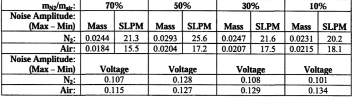
The four figures 8a, 8b, 8c, and 8d show a fair amount of noise and variation present in the controlled flow, especially as the flow's value decreases. The coefficients of variation of the two flows also show the increasing significance of noise as flows fall, as shown in Figure 9. Much of this is simply due to scaling effects, because the flow controller's output voltage is proportional to the amount of flow that is passing through the device, while the noise is of roughly constant amplitude, as shown in Table 2 below.

mN2/mar: 70% 50% 30% 10%

Noise Amplitude:

(Max -Min) Mass SLPM Mass SLPM Mass SLPM Mass SLPM N2: 0.0244 21.3 0.0293 25.6 0.0247 21.6 0.0231 20.2

Air: 0.0184 15.5 0.0204 17.2 0.0207 17.5 0.0215 18.1 Noise Amplitude:

(Max - Min) Voltage Voltage Voltage Voltage

N2: 0.107 0.128 0.108 0.101

Air: 0.115 0.127 0.129 0.134

Table 2: Noise amplitude data taken during testing at an engine speed of 2200 rpm.

Values are taken from the 80th recorded data point (8 seconds from the start of recording) onward so that skewing of the data due to transient start-up effects is avoided.

(29)

Assuming a perfect controller with no lag between measurement of the air flow and adjustment of the diluent flow, infinitesimal rise and settling times, and perfect, noiseless sensor readings, the coefficient of variation of the air and N2 flows would be

equal. Any variation in air flow would be perfectly mirrored by variation in N₂flow, thus giving the two flows the same statistical properties. However, a real controller is not perfect. Due to the controller's tendency to overshoot its set point slightly and also due to its non-zero settling time the N2 flow will likely have slightly more variance than the

air flow as the controller attempts to keep the two in constant proportion, but the two results should be fairly comparable assuming minimal noise.

In this case, however, noise represents a large percentage of the total signal for low flow rates. The absolute variance stays relatively constant between the four flow ratios even as the signal amplitude falls, thus causing the lower flow rates to have more relative variance than the higher flows do. This causes the coefficient of variation to rise significantly for lower flow rates, though not necessary because the flow is less controlled.

As shown in Table 2, the noise amplitude for the N2 flows is generally a little

larger than that of the air flow. This increase is likely due to a combination of the controller properties as discussed above and noise in the signal. Although the signal coming from the flow controller has less voltage variation in an absolute sense than the signal coming from the air flow sensor, these variations represent a larger percentage of its respective signal and so can cause larger flow variation.

(30)

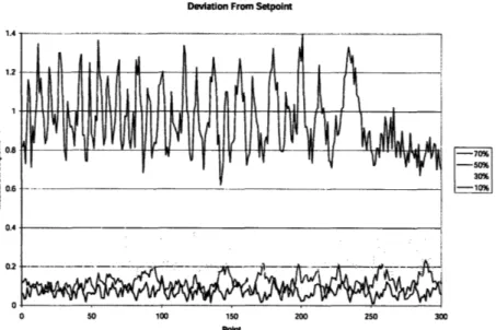
Deviation From Setpoint 1.4 12 1 70.8 0.6 0.4 0.2 0 70% -50% 30% -10% 0 50 100 150 200 250 300 Point

Figure 10: _{The actual flow's deviation from the set point value given to the controller,}

defined as measured/requested - 1. The last 300 points (30 seconds) of each test run are taken to ensure the absence of transient behavior.

Shown above in Figure 10, the deviation of the actual flow from the set point given to the flow controller remains relatively constant during the experiment. This shows that the flow controller can control flows with good precision, but its accuracy is less than ideal.

Smoothed Deviation From Setpoint 1.4 1.2. 1 0.8 0.64 0.4 0.2 0

...

7...t

f.

...

....

..

...

..

...

70% 50% 30% -10% 0 50 100 150 200 250 300 Point

Figure 11: Smoothed version of the actual flow's deviation from the set point value

given to the controller, defined as measured/requested - 1. This version averages each point with the 4 immediately preceding points to help reduce noise and clarify trends.

--- h/2ln /~~nM~\rr~L~-~/U

(31)

mN2/m: Step Response 70% 50% 30% 10%

SLPM

N2: 207.4 154.8 123.1 92.1 53.8

Air: - 199.6 212.5 238.4 263.5

Mass Flow [kg/min]

N2: 0.2375 0.1773 0.1410 0.1055 0.0616

Air: - 0.2363 0.2516 0.2823 0.3120

Actual Percentage: - 75.01 56.05 37.37 19.74

Error [%]: 3.72 7.16 12.09 24.56 97.40 Error [kg/min]: 0.0085 0.0118 0.0152 0.0208 0.0304

Table 3: Flow data taken during testing. The flow ratio data was taken at an engine

speed of 2200 rpm, while the step response data was taken while the engine was off. Values for the flow ratio data are averaged from the 80th recorded data point (8 seconds

from the start of recording) onward and values for the step response data are averaged from the 41 st data point (4.1 seconds) after the step impulse onwards, to avoid any

skewing of the data from transient behavior.

The flow controller in its current state has a very difficult time keeping low flow rates close to the values called for by the LabView VI. As shown in Table 3, the flow rates for all data points taken were below the recommended 250 SLPM rating given by the manual [5]. Steady state error increases rapidly as flow rate decreases until the actual flow is nearly twice what it needs to be for a N2/air flow ratio of 10%.

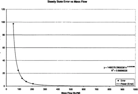
Steady State Error vs Mass Flow

80 io 40 20 y - 1466379.39650361x-" L 4 s s3e - 0.99896028 +Error; -- Power (Error) 0 100 200 300 400 500 600 700 800 900 1000 Mass Flow [SL.PM

Figure 12: Steady State Error between actual flow and

of mass flow in SLPM.

controller set point as a function

--- i

'"

(32)

When steady state error is plotted against mass flow, a clear trend is seen. A power regression performed on the data by Excel yields an equation of the following type that describes the error to a high degree of accuracy:

Es = a * SLPMb (5)

where Ess is the steady state error, a is equal to 1466379.39650361, SLPM is the mass flow rate in SLPM as measured by the flow controller, and b is equal to -2.42355398. This equation fits the data with an R2 _{value of 0.99896028, showing that it describes the}

acquired data very well. Equation (5) can be used to predict steady state error for various values of mass flow. Attempting to flow N2 gas at the minimum rating of 250 SLPM of

the flow controller [5] would result in a steady state error of just 2.26%, and the error falls below 1% at flow rates greater than 350 SLPM. Further research is necessary to confirm the equation's accuracy at these higher mass flow rates, but it would make sense that the flow controller's steady state error is quite low in the range for which it was designed.

(33)

Chapter 4 Conclusion

The objective of this experiment was to provide an experimental set up and computer program to allow the control of fuel and diluent gas flows based on a percentage of measured intake air flow to an engine. The experimental set up should allow for the user to select the air-fuel and air-diluent gas ratios so a wide range of operating conditions can be tested. This will allow the characterization of a diesel engine running in the fuel rich Low-Temperature-Combustion mode. Information gathered from this study will be useful in determining the feasibility of a hybridized diesel engine, intermediate temperature solid oxide fuel cell powertrain for long haul trucks, a combination that theoretically has the capability of significantly raises overall system efficiency without subjecting the vehicle operator to the drawbacks of a stand-alone fuel cell power unit.

4.1: Summary

The project undertaken for this thesis resulted in the creation of an experimental set up that allows the operation of and collection of data about air, fuel, and diluent gas flows into a diesel engine running in the fuel rich Low-Temperature-Combustion mode. Verification of the effectiveness of this set up was also carried out. This was done by examining three vital system operations- its ability to accurately and predictably control rotational speed of the motored diesel engine, its flow controller step response characteristics, and its ability to control nitrogen gas flow, a stand-in for the diluent gas mixture to be used in later experiments, at 10%, 30%, 50%, and 70% mass fraction of the intake air flow.

The engine speed was controlled using a dynamometer coupled to the engine's driveshaft via an electromagnetic clutch. The clutch lockup was varied by supplying a current to the device using a standard power supply. The clutch lockup, and thus the torque transmitted to the engine, is a function of this clutch coil current. The engine speed should also be proportional to the clutch coil current, since the torque is

(34)

theoretically constant for a given clutch lockup, but this is not the case. Over a period of approximately 30 minutes, engine speed dropped 17% for a given clutch coil current. This deviation is likely to have been caused by either an oil leak that started during the test runs or an overheated dynamometer, which was not externally cooled during this experiment. Further testing is required to determine the true source of this unforeseen variation.

The flow controllers step response showed it to be up to the task of controlling a steady state flow on the time scale of engine acceleration, as long as flow values are high enough. When encountering a step impulse, the controller exhibited a 10%-90% rise time of 0.19 seconds, took 1.7 seconds to settle to within 5% of its steady state value, had a 3.1% overshoot, and had a steady state error of 3.7%. The rise time, settling time, and overshoot will be more than adequate for this experiment, which is taking place under steady state conditions. The steady state error is likely due to the low flow rate of 207.4 SLPM the flow controller is attempting to meter, which is 17% below the flow controller's rated minimum flow of 250 SLPM. More will be mentioned on this topic in the following paragraph on feedback flow control.

When feedback flow control is enabled, the controller exhibits the ability to maintain flow within approximately 0.015 kg/min of the mean flow. However, this value is relatively constant for all flow rates, varying between about 0.011 kg/min to 0.015 kg/min for the flow values analyzed, which ranged from approximately 0.06 kg/min to 0.18 kg/min. The flow variation, then, represents a much greater percentage of the mean flow when mass flow values are low than it does when mass flow values are high. Much of this error is simply due to noise in the signal and variations of the measured intake air. However, some of it is likely due to slight controller overshoot when the flow set point changes due to intake air flow variation, which happens constantly while the experiment is being run.

The increasing significance of variance is not the only problem facing the control of low flow rates. The particular controller being used, a FMA-2613A Mass Flow Controller made by Omega Engineering, Inc., is only rated for flows between 250 SLPM and 1000 SLPM, or nitrogen mass flows between 0.35 kg/min and 1.145 kg/min. The flows being examined in this experiment are typically well below the lower bound of these values. The percent steady state error present in the controlled fluid increases faster

(35)

than the relative change in flow rate to the -2.4 as flow rates decrease from 250 SLPM, resulting in nearly 100% steady state error for desired flow rates of 0.03 kg/min, or around 10% air-N2 flow ratio at 2200 rpm. Since flows of this ratio should be accurately

controlled for the collection of accurate data representative of the engine operating characteristics over a wide range of conditions, something must be done to rectify this situation. Either a new controller should be chosen or a set point offset should be applied using the controlling software on a PC, assuming the same engine is to be used.

4.2: Future Work

The experimental set up and methods presented above provide a solid foundation on which future experimentation can build. However the setup must be fine tuned before final experiments can take place. The engine's oil leak should be repaired, and the dynamometer should be connected to an external cooling source so that engine speed can be reliably controlled via the clutch coil current. The flow controller's transient behavior should be examined in greater depth and any necessary changes should be made. Steady state error at low flow rates should be dealt with, either through the use of negative offsets calculated by the LabView control program through the use of Eq. (5), the equation that gives the relation between steady state error and flow rates for flows of less than 250 SLPM, or through the implementation of a faster acting PI controller in the LabView environment to supply its own offset. System performance will change, however, so care should be taken to redxamine the controller characteristics if a separate PI loop is added. A new flow controller that is rated for flows of this level, between 50 and 200 SLPM, could also be chosen to replace the current controller, which would eliminate the need for software compensation for this problem.

After these issues are taken care of, the next steps to be followed are already laid out in references [2] and [3]. Fuel control should be implemented, with fuels of either propane or n-heptane having been suggested, and the true diluent gas, a mixture of CO2,

N2, H2, and CO, should replace the nitrogen currently being used as diluent. It was also

suggested that the compression ratio be lowered to 15.5:1 from its current value of 19.5:1. Once these steps have been taken, the experimental preparation will be complete.

(36)

(37)

References

[1] Cheng, Wai K. "Phase 1 Proposal to Eaton Corporation." March 31, 2005. Unpublished.

[2] Cheng, Wai K. "Phase 2 Proposal to Eaton Corporation." October 20, 2005. Unpublished.

[3] Cheng, Wai K., and Hahn, Tairin. "Assessment of Low-Temperature-Combustion Diesel Engine as an On-Board Reformer for ITSOFC Powered Vehicle." Date Unknown. Unpublished.

[4] Omega Engineering, Inc. "User's Guide: FMA-900 Series Air Velocity Transducers." 2005.

[5] Omega Engineering, Inc. "User's Guide: FMA-2600A/FVL-2600A Series Mass and Volumetric Flow Controllers." 2001.

(38)

Appendix A: Engine Speed vs. Current

Voltage Current RPM First Test 18.5 0.31 1792 19 0.32 2002 20 0.34 2173 21 0.36 2292 22 0.38 2445 23 0.4 2547 24 0.42 2619 Second Test 18.5 0.31 1752 19 0.32 1901 20 0.34 2015 21 0.36 2134 22 0.38 2227 23 0.4 2352 24 0.42 2471 25 0.44 2573 26 0.46 2657 27 0.48 2724 28 0.51 2797 29 0.53 2865 Third Test 24 0.42 2345 25 0.44 2452 25.5 0.45 2521 26 0.46 2586 26.5 0.47 2625 27 0.48 2662 27.5 0.49 2693 28 0.51 2716

During Engine Tests 24 0.42 2220

23.9 0.42 2195 24 0.42 2186 24.5 0.43 2202

(39)

Appendix B: Controller Set Point vs.

Input Voltage

Input Voltage [VDC] Set Point [SLPM]

0 0 0.5 101 1 201 1.5 301 2 401 2.5 501 3 601 3.5 701 4 801 4.5 901 5 1001