Convex optimization methods for graphs and statistical modeling

(1)

Convex Optimization Methods for

Graphs and Statistical Modeling

by

Venkat Chandrasekaran

B.A. in Mathematics, B.S. in Electrical and Computer Engineering Rice University (2005)

S.M. in Electrical Engineering and Computer Science Massachusetts Institute of Technology (2007)

MASSACHUSETTS INSTITUTE OF TECHNOLOGY

JUN 17 2011

LIBRARIES

o-visor

Accepted by:

n)u~fr.

noumuejski

Professor of Electrical Engineering and Computer Science Chair, Department Committee on Graduate Students

(2)

(3)

Convex Optimization Methods for

Graphs and Statistical Modeling

by Venkat Chandrasekaran

Submitted to the Department of Electrical Engineering and Computer Science on April 29, 2011

in Partial Fulfillment of the Requirements for the Degree

of Doctor of Philosophy in Electrical Engineering and Computer Science

Abstract

An outstanding challenge in many problems throughout science and engineering is to succinctly characterize the relationships among a large number of interacting enti-ties. Models based on graphs form one major thrust in this thesis, as graphs often provide a concise representation of the interactions among a large set of variables. A second major emphasis of this thesis are classes of structured models that satisfy certain algebraic constraints. The common theme underlying these approaches is the develop-ment of computational methods based on convex optimization, which are in turn useful in a broad array of problems in signal processing and machine learning. The specific contributions are as follows:

" We propose a convex optimization method for decomposing the sum of a sparse

matrix and a low-rank matrix into the individual components. Based on new rank-sparsity uncertainty principles, we give conditions under which the convex program exactly recovers the underlying components.

" Building on the previous point, we describe a convex optimization approach to

latent variable Gaussian graphical model selection. We provide theoretical guar-antees of the statistical consistency of this convex program in the high-dimensional scaling regime in which the number of latent/observed variables grows with the number of samples of the observed variables. The algebraic varieties of sparse and low-rank matrices play a prominent role in this analysis.

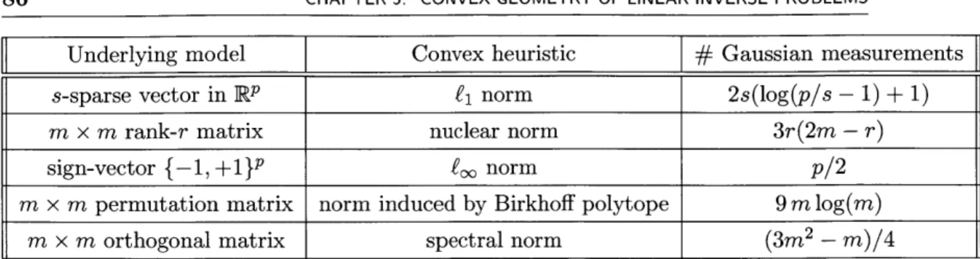
" We present a general convex optimization formulation for linear inverse problems,

in which we have limited measurements in the form of linear functionals of a signal or model of interest. When these underlying models have algebraic structure, the

(4)

resulting convex programs can be solved exactly or approximately via semidefinite programming. We provide sharp estimates (based on computing certain Gaussian statistics related to the underlying model geometry) of the number of generic linear measurements required for exact and robust recovery in a variety of settings.

e

We present convex graph invariants, which are invariants of a graph that are con-vex functions of the underlying adjacency matrix. Graph invariants characterize structural properties of a graph that do not depend on the labeling of the nodes; convex graph invariants constitute an important subclass, and they provide a sys-tematic and unified computational framework based on convex optimization for solving a number of interesting graph problems.

We emphasize a unified view of the underlying convex geometry common to these different frameworks. We describe applications of both these methods to problems in financial modeling and network analysis, and conclude with a discussion of directions for future research.

Thesis Supervisors: Alan S. Willsky and Pablo A. Parrilo

(5)

Acknowledgments

I have been truly lucky to have two great advisors in Alan Willsky and Pablo Parrilo. I am extremely grateful to them for giving me complete freedom in pursuing my interests

while also providing research guidance, for sharing with me their tremendous intellectual enthusiasm and curiosity, for reading our paper drafts promptly, and for the countless conversations about research, jobs and life. Thanks, Pablo and Alan, for everything.

I am very grateful to Devavrat Shah for his many words of encouragement and

advice, and for serving on my thesis committee. My thanks also go to Sanjoy Mitter for his support at various stages during my time at MIT.

I enjoyed working with many wonderful researchers these last few years. This thesis

is the result of some of these collaborations. In addition to Pablo, Alan, and Devavrat.,

I would like to thank Jin Choi, Ben Recht, Jason Johnson, Parikshit Shah, Dmitry

Malioutov, James Saunderson, Ying Liu, Anima Anandkumar, Jinwoo Shin, David Gamarnik, Misha Chertkov, Sujay Sanghavi, Nathan Srebro, and Prahladh Harsha.

I am grateful to Rachel Cohen, Debbie Deng, Jennifer Donovan, Janet Fischer, Lisa

Gaumond, and Brian Jones for their assistance in ensuring that my progress through MIT was smooth.

I could not have asked for a better set of people with whom to interact than those in LIDS: Jason Johnson, Jason Williams, Dmitry Malioutov, Pat Kreidl, Ayres Fan, Emily Fox, Jin Choi, Kush Varshney, Ying Liu, James Saunderson, Matt Johnson, Vincent Tan, Anima Anandkumar, Peter Jones, Lav Varshney, Parikshit Shah, Amir Ali Ahmadi, Noah Stein, Ozan Candogan, Mesrob Ohannessian, Srikanth Jagabathula, Jinwoo Shin, Hari Narayanan, Shashi Borade, and many others. Outside of LIDS, I'm very lucky to be able to count Shrini Kudekar, Rene Pfitzner, Urs Niesen, Evgeny Logvinov, Ryan Giles, and Matt Barnett as my friends.

Finally I would like to thank my family for their love, support, and encouragement. Funding: This research was supported in part by the following grants - MURI AFOSR grant FA9550-06-1-0324, MURI AFOSR grant FA9550-06-1-0303, NSF FRG

(6)

(7)

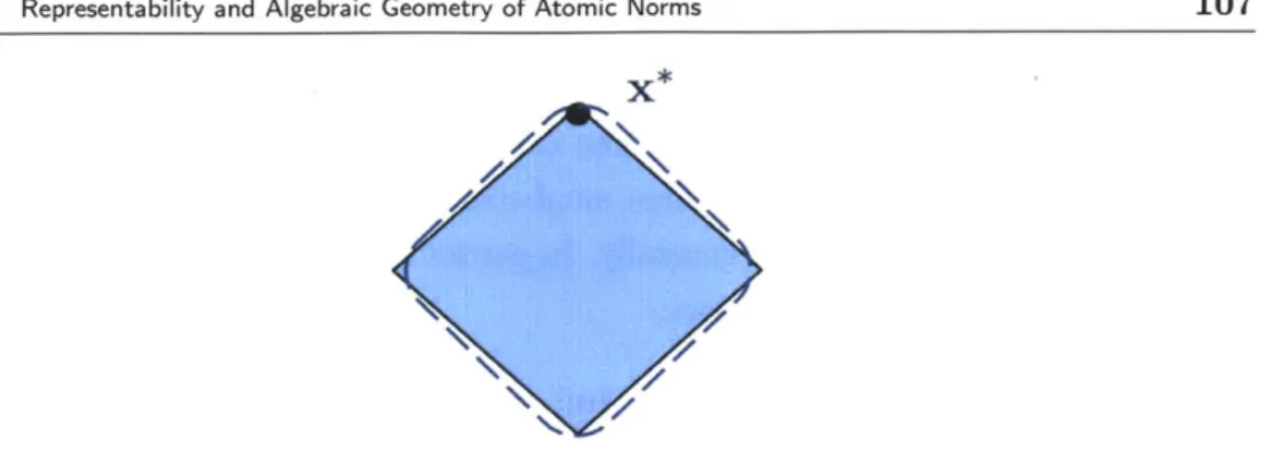
5.4 Representability and Algebraic Geometry of Atomic Norms 5.4.1 Role of algebraic structure . . . . 5.4.2 5.4.3 . . . . 87 . . . . 87 . . . . 89 . . . . 92 . . . . 93 . . . . 94 . . . . 95 . . . . 96 . . . . 98 . . . 100 . . . 102 . . . 105 . . . 105

Semidefinite relaxations using Theta bodies - an example Tradeoff between relaxation and number of measurements 107 108 5.4.4 Terracini's lemma and lower bounds on recovery . . . 111

5.5 Computational Experiments . . . 113

5.5.1 Algorithmic considerations . . . 113

5.5.2 Simulation results . . . 115

5.6 D iscussion . . . 117

6 Convex Graph Invariants 119 6.1 Introduction . . . 119

6.2 A pplications . . . 123

6.2.1 Graph deconvolution . . . 124

6.2.2 Generating graphs with desired structural properties . . . 125

6.2.3 Graph hypothesis testing . . . 126

6.3 Convex Graph Invariants . . . 127

6.3.1 Motivation: Graphs and adjacency matrices . . . 127

6.3.2 Definition of convex invariants . . . 128

6.3.3 Examples of convex graph invariants . . . 130

6.3.4 Examples of invariant convex sets . . . 133

6.3.5 Representation of convex graph invariants . . . 135

(10)

10 CONTENTS

6.3.7 Comparison with spectral invariants . . . .

6.3.8 Convex versus non-convex invariants . . . . 6.4 Computing Convex Graph Invariants . . . .

6.4.1 Elementary invariants and the Quadratic Assignment problem 6.4.2 Other methods and computational issues . . . .

6.5 Using Convex Graph Invariants in Applications . . . .

6.5.1 Application: Graph deconvolution . . . .

6.5.2 Application: Generating graphs with desired properties . . . . .

6.5.3 Application: Graph hypothesis testing . . . .

6.6 D iscussion . . . . 7 Conclusion 7.1 Summary of Contributions . . . . 7.2 Future Directions . . . . A Proofs of Chapter 3 A.1 SDP Formulation . . . . A .2 Proofs . . . . B Proofs of Chapter 4

B.1 Matrix Perturbation Bounds B.2 Curvature of Rank Variety . . . .

B.3 Transversality and Identifiability B.4 Proof of Main Result . . . .

B.4.1 B.4.2 B.4.3 B.4.4 B.4.5 B.4.6 B.4.7

Bounded curvature of mat Bounded errors . . . . Solving a variety-constrair From variety constraint to Removing the tangent-spa Probabilistic analysis . . . Putting it all together . .

157 . . . 157 . . . 158 161 . . . 16 1 . . . 16 1 171 . . . 17 1 . . . 173 . . . 175 . . . 177 rix inverse . . . 179 . . . 180 ed problem . . . 183 tangent-space constraint . . . 186 ce constraints . . . 189 . . . 19 1 . . . 19 2 C Proofs of Chapter 5 C.1 Proof of Proposition 5.3.1 . . . . C.2 Proof of Theorem 5.3.3 . . . . 197 . . . 197 . . . 198 140 141 142 142 144 145 145 149 152 154

(11)

CONTENTS 11

C.3 Direct W idth Calculations . . . 201

D Properties of Convex Symmetric Functions 207

(12)

(13)

Chapter 1 Introduction

An outstanding challenge in many applications throughout science and engineering is to succinctly characterize the relationships among a large number of interacting entities. In a statistical model selection setting we wish to learn a "simple" statistical model to approximate the behavior observed in a collection of random variables. Modern data analysis tasks in geophysics, economics, and image processing often involve learning sta-tistical models over collections of random variables that may number in the hundreds of thousands, or even a few million. In a computational biology setting a typical question involving gene regulatory networks is to discover the interaction patterns among a col-lection of genes in order to better understand how a gene influences or is influenced by other genes. Similar problems also arise in the analysis of biological, social, or chemical reaction networks in which one seeks to better understand a complicated network by decomposing it into simpler networks. Models based on graphs offer a fruitful frame-work to solve such problems, as graphs often provide a concise representation of the interactions among a large set of variables.

In this thesis we explore a set of research directions at the intersection of graphs and statistics. An important instance of a framework that lies in this intersection is that of graphical models, in which a statistical model is defined with respect to a graph. Another example is one in which we have statistical models over the space of graphs, so that a graph itself is viewed as a sample drawn from a probability distribution defined over some set of graphs. Natural questions that arise in standard statistical settings such as deconvolution can then be posed in a deterministic framework in this graph setting as well.

A common theme underlying our investigations is the development of tractable

computational tools based on convex optimization, which possess numerous favorable properties. Due to their powerful modeling capabilities, convex optimization methods

(14)

CHAPTER 1. INTRODUCTION can provide tractable formulations for solving difficult combinatorial problems exactly or approximately. Further convex programs may often be solved effectively using general-purpose off-the-shelf software. Finally one can also give conditions for the success of these convex relaxations based on standard optimality results from convex analysis.

U

1.1 Main Contributions

In this section we outline the main contributions of this thesis. Details about related previous work are given in the relevant chapters. The research and results of Chapters 3, 4, 5, and 6 correspond to the papers [37], [33], [36], and [34] respectively.

Rank-Sparsity Uncertainty Principles and Matrix Decomposition

Suppose we are given a matrix that is formed by adding an unknown sparse matrix to an unknown low-rank matrix. The goal is to decompose the given matrix into its sparse and low-rank components. Such a problem is intractable to solve in general, and arises in a number of applications such as model selection in statistics, system identification in control, optical system decomposition, and matrix rigidity in computer science. In-deed sparse-plus-low-rank matrix decomposition is the main challenge in latent-variable Gaussian graphical model selection, which is discussed next (and in greater detail in Chapter 4). In Chapter 3, we propose a convex optimization formulation to splitting the specified matrix into its components, by minimizing a linear combination of the f norm and the nuclear norm (the sum of the singular values of a matrix) of the components. We develop a notion of rank-sparsity incoherence, expressed as an uncertainty principle between the sparsity pattern of a matrix and its row and column spaces, and use it to characterize both fundamental identifiability as well as (deterministic) sufficient condi-tions for exact recovery. The analysis is geometric in nature with the tangent spaces to the algebraic varieties of sparse and low-rank matrices playing a prominent role.

Latent Variable Gaussian Graphical Model Selection

Graphical models are widely used in many applications throughout machine learning, computational biology, statistical signal processing, and statistical physics as they offer a compact representation for the statistical structure among a large collection of random variables. Graphical models in which the underlying graph is sparse typically tend to be better suited for efficiently performing tasks such as inference and estimation.

(15)

Sec. 1.1. Main Contributions 15

In the setting of Gaussian graphical models where the random variables are jointly Gaussian, sparsity in the graph structure corresponds to sparsity in the inverse of the covariance matrix of the random variables, also called the concentration matrix. Thus Gaussian graphical model selection is the problem of learning a model described by a sparse concentration matrix to best approximate the observed statistics in a collection of random variables [119]. However a significant difficulty arises if we do not have sample observations of some of the relevant variables, because a whole set of extra correlations

are induced among the observed variables due to marginalization over the unobserved, hidden variables. Is it possible to discover the number of hidden components, and to learn a statistical model over the entire collection of variables? If only we realized that much of the seemingly complicated correlation structure among the observed variables can be explained as the effect of marginalization over a few hidden variables, we would be able to learn a "simple" statistical model among the observed variables and a few

additional hidden variables.

In the Gaussian setting this problem reduces to one of approximating a given matrix

by the sum of a sparse matrix and a low-rank matrix: the low-rank matrix corresponds

to the correlations induced by marginalization over latent variables (it is low-rank as the number of hidden variables is usually much smaller than the number of observed vari-ables), and the sparse matrix corresponds to the conditional graphical model structure among the observed variables conditioned on the latent variables. From a statistical viewpoint this approach to modeling can be seen as a blend of dimensionality reduction (to identify latent variables) and graphical modeling (to capture remaining statistical structure not attributable to the latent variables). In Chapter 4, we propose a tractable convex programming estimator for latent variable Gaussian graphical model selection based on regularized maximum-likelihood; motivated by the results in Chapter 3 the regularizer uses the f, norm for the sparse component, and the nuclear norm for the low-rank component. In addition to being computationally efficient to evaluate, this estimator enjoys favorable statistical consistency properties. Indeed we show that con-sistent model selection is possible under suitable identifiability conditions even if the number of observed/latent variables is on the same order as the number of samples of the observed variables. The rank-sparsity uncertainty principles of Chapter 3 described above are fundamental to our analysis. Previous approaches to latent variable graphical modeling using variants of the Expectation-Maximization (EM) algorithm do not share these favorable properties, as they optimize non-convex functions (hence converging

(16)

CHAPTER 1. INTRODUCTION

only to local optima) and have no high-dimensional consistency guarantees.

Convex Optimization for Inverse Problems

Many of the questions from the previous two sections can be viewed as instances of inverse problems in which we wish to recover simple and structured models given limited information. In Chapter 5 we study a general class of linear inverse problems in which the goal is to recover a model given a small number of linear measurements. Such problems are generally ill-posed as the number of measurements available is typically smaller than the dimension of the model. However in many practical applications of interest, models are often constrained structurally so that they only have a few degrees of freedom relative to their ambient dimension. Exploiting such structure is the key to making linear inverse problems well-posed. The class of simple models that we consider in Chapter 5 are those formed as the sum of a few atoms from some elementary atomic set; examples include well-studied cases such as sparse vectors (e.g., signal processing, statistics) and low-rank matrices (e.g., control, statistics), as well as several others such as sums of a few permutations matrices (e.g., ranked elections, multiobject tracking), low-rank tensors (e.g., vision, neuroscience), orthogonal matrices (e.g., machine learning), and atomic measures (e.g., system identification). We describe a general framework to convert such notions of simplicity into convex penalty functions, which give rise to convex optimization solutions to linear inverse problems. These convex programs can be solved via semidefinite programming under suitable conditions, and they significantly generalize previous approaches based on i norm and nuclear norm minimization for recovering sparse and low-rank models. Our results give general conditions and bounds on the number generic measurements under which exact or robust recovery of the underlying model is possible via convex optimization. Thus this work extends the catalog of simple models (beyond sparse vectors, i.e., compressed sensing, and low-rank matrices) that can be recovered from limited linear information via tractable convex programming.

Convex Graph Invariants

Investigating graphs from the viewpoint of statistics provides a very fruitful research agenda, as many questions from classical statistics can be posed in a deterministic setting in which data are represented as graphs. As an example suppose that we have a composite graph formed as the combination of two graphs

gi

and G2 overlaid on

(17)

Sec. 1.1. Main Contributions 17

the same set of nodes. We are only given the composite graph without any additional information about the relative labeling of the nodes, which may reveal the structure of the individual components. Can we deconvolve the composite graph into the individual components? As discussed in Chapter 6 such a problem is of interest in network analysis in social and biological networks in which one seeks to decompose a complex network into simpler components to better understand the behavior of the composite network. Other problems motivated by statistics include hypothesis testing between families of graphs, and generating/sampling graphs with certain desired structural properties (see Chapter 6 for details).

An important goal towards solving these and many other graph problems is to characterize the underlying structural properties of a graph. Graph invariants play an important role in describing such abstract structural features, as they do not depend on the labeling of the nodes of the graph. Examples of commonly used graph invariants include the spectrum of a graph (i.e., eigenvalues of the adjacency matrix), or the degree sequence. In Chapter 6 we introduce and investigate convex graph invariants, which are graph invariants that are convex functions of the adjacency matrix of a graph. Examples of such functions of a graph include the maximum degree, the MAXCUT value (and its semidefinite relaxation), the second smallest eigenvalue of the Laplacian, and spectral invariants such as the sum of the k largest eigenvalues of the adjacency matrix. Convex graph invariants provide a systematic and unified computational framework based on convex optimization for solving a number of interesting graph problems such as those described above.

(18)

(19)

Chapter 2 Background

In this chapter we emphasize the main themes common to the rest of this thesis. Our exposition is brief as we only provide the basic relevant technical background, and we refer the reader to the texts [124] (on convex analysis) and

[79]

(on algebraic geometry) for more details. The individual chapters also give more background pertaining to the corresponding chapter.

* 2.1 Basics of Convex Analysis

A set C C RP is a convex set if for any x, y E C and any scalar A E [0, 1], we have that Ax + (1 - A)y E C. A convex set C is also a cone if it is closed under positive linear

combinations. Such convex cones are fundamental objects of study in convex analysis, and play an important role in all the main chapters of this thesis.

The polar C* of a cone C is the cone

C* = {x E RP : (x, z) < 0 Vz E C}.

Given a closed convex set C E RP and some nonzero x E RP we define the tangent cone at x with respect to C as

Tc(x) = cone{z - x : z C}. (2.1)

Here cone(-) refers to the conic hull of a set obtained by taking nonnegative linear combinations of elements of the set. The cone Tc (x) is the set of directions to points in C from the point x. The normal cone Nc(x) at x with respect to the convex set C is defined to be the polar cone of the tangent cone Tc(x), i.e., the normal cone consists of vectors that form an obtuse angle with every vector in the tangent cone Tc(x).

(20)

20 CHAPTER 2. BACKGROUND

if for any x, y

E

C and any scalar A E [0, 1], we have that

f(Ax + (1 - A)y) < Af(x) + (1 - A)f(y).

Following standard notation in convex analysis, we denote the subdifferential of a convex

function

f

at a point k in its domain by Of(k). The subdifferential

af(i)

consists of

all y such that

f (x)

>

f (k) + (y,x

- k), Vx.

M

2.2 Representation of Convex Sets

Convex programs denote those optimization problems in which we seek to minimize a convex function over a convex constraint set [24]. For example linear programming and semidefinite programming form two prominent subclasses in which linear functions are minimized over constraint sets given by affine spaces intersecting the nonnegative orthant (in linear programming) and the positive-semidefinite cone (in semidefinite programming) [11]. Roughly speaking convex programs are tractable to solve compu-tationally if the convex objective function can be computed efficiently, and membership in the convex constraint sets can be certified efficiently. Hence, the tractable represen-tation of convex sets is an important point that must be addressed in order to develop practically feasible computational solutions to convex optimization problems.

Any closed convex set has two dual representations. Specifically, an element x be-longing to a convex set C is an extreme point if it cannot be expressed as the midpoint of the line segment between some two points in C. With this definition the first repre-sentation of a convex set is as the convex hull of all its extreme points. With respect to this representation, certifying membership in a convex set means that we must produce a representation of a point as the convex combination of (a subset of) extreme points. A second representation of a convex set is as the intersection of (possibly infinitely many) halfspaces. Here certifying membership of a point in a convex set means that we need to verify that this point satisfies the constraints defining the convex set. Using the tools of convex duality one can transform between these two alternate representations of a convex set (see [124] for more details).

In this section we provide several examples of convex sets and their representations, with the objective of highlighting the main ideas that lead to tractable representations. In particular the concept of lift-and-project plays a central role in many examples of efficient representations of convex sets. The lift-and-project concept is simple - we wish

(21)

Sec. 2.2. Representation of Convex Sets 21

11

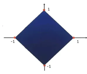
Figure 2.1. The cross-polytope in two dimensions.

to express a convex set C E RP as the projection of a convex set C' E RP' in some higher-dimensional space (i.e., p' > p). Such methods are useful if p' is not too much larger than p and if C' has an efficient representation in the higher-dimensional space RP'. Lift-and-project provides a very powerful representation tool, as will be seen in the examples to follow.

M

2.2.1 Cross-polytope

The cross-polytope (see Figure 2.1) is the unit ball of the e1-norm:

BP

=

{x

E RP

|

lxii

<

1.

The fi-norm has been the focus of much attention recently due to its sparsity-inducing properties [29,53,54].

In a statistical model selection setting sparsity corresponds to models that consist of few nonzero parameters. Specialized to a linear regression or feature selection context, penalty functions based on the ei-norm lead to parameter vectors that are sparse, i.e., responses are expressed as the linear combination of a small number of features

[135]. Specialized to a covariance selection context, fi-norm penalty functions lead

to distributions defined by sparse covariance and concentration matrices [15, 16, 61]. Sparsity has also played a central role in signal processing as a variety of applications exploit the expression of signals as the sum of few elements from a dictionary, e.g.,

(22)

22 CHAPTER 2. BACKGROUND approximating natural images as the weighted sum of a few wavelet basis functions. The benefits of such sparse approximations are clear for tasks such as compression, but extend also to tasks such as signal denoising and classification.

How do we represent the p-dimensional cross-polytope B ? While the cross-polytope has 2p vertices, a direct specification in terms of halfspaces involves 2P inequalities:

B = x c RP | zixi 1, Vz E {-1- +}P}.

However we can obtain a tractable inequality representation by lifting to R2P and then projecting onto the first p coordinates:

B = x E RP

I

3z E RP s.t. - zi xi < z Vi, zi < 1, zi > 0 Vi}.

Note that in R2p with the additional variables z, we have only 3p

+

1 inequalities.

Next suppose x E B is a point on the boundary of the cross-polytope, i.e., |xIle,

1. Letting Q

{1,

... ,p} denote the indices at which x is nonzero, the normal cone at

x with respect to BP, is given as:

NBP (x) = {z I zi = tsgn(xi) for i E 2,

Izil

I t for i c Qc for some t > 0}.

Here sgn(.) is the sign function.

M

2.2.2 Nuclear-norm ball

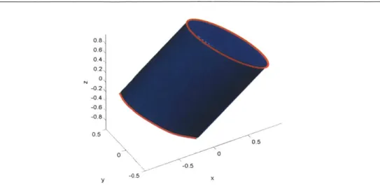
The nuclear norm of a matrix (see Figure 2.2 for the unit ball) is the sum of its singular values:

IlXIlI, = Zui(X).

i

Analogous to the case of the fl-norm, the nuclear norm has received much attention recently because it induces low-rank structure in matrices in a number of settings [30, 121].

In a statistics context low-rank covariance matrices are used in factor analysis, and they represent the property that the corresponding random variables lie on or near a low-dimensional subspace. In a control setting low-rank system matrices correspond to systems with a low-dimensional state space, i.e., systems with small model order. In optical system modeling low-rank matrices represent so-called coherent systems, which correspond to low-pass optical filters.

(23)

Sec. 2.2. Representation of Convex Sets 0.8, 0.6 0.4, 0.2, 0 -0.2 s -0.4, -0.6 -0.8 . 0.5 0.5 0 - 0 -0.5 -0.5 X

Figure 2.2. The nuclear-norm ball of 2 x 2 symmetric matrices. Here x, y denote the diagonal entries, and z the off-diagonal entry.

Unlike with the f1-norm the nuclear-norm of a matrix has no closed-form

represen-tation, but can instead be expressed variationally. Specifically, the spectral or operator norm 1| - || of a matrix (the largest singular value) is the dual norm of the nuclear-norm

|| - | [82]:

|IX||,

= max{Tr(X'Y)I

IIYII

1}.

Further, the spectral norm admits a simple semidefinite characterization:

||Yl|= min t s.t. > 0.

t ₍ _Y' _tIn

We then obtain the following SDP characterization of the nuclear-norm:

X||, = min 1(trace (Wi) + trace(W2))

W1,W2 2

W1 X

s.t. >-W0.

(X' W2

This semidefinite characterization can in turn be used to specify the unit ball of the nuclear-norm:

B Px

{X

E RPXP | ||X||, < 1} .

Suppose X E BP is a boundary point of the nuclear-norm ball, i.e., ||X||, = 1.

(24)

CHAPTER 2. BACKGROUND

l23 141

12111 1 1 .2

V121] 12

132 1

Figure 2.3. The permutahedron generated by the vector [1, 2,3,4]'.

and E E Rrank(X)xrank(X). Further let W C RPxP denote the subspace of matrices given by the span of matrices with either the same row space or the same column space as X:

W=

{UM'+

NV' I M, N E Rpxrank(X)

Then we have the following description of the normal cone at X with respect to BPxP: NPxp(X)

{tUVT

+ WE RPXP WTU =0,WV = 0,

IIWI|

< t,t ;>0}.

Here P denotes the projection operator. Notice the parallels with the normal cone with respect to the cross-polytope.

M

2.2.3 Permutahedron

The permutahedron (see Figure 2.3) generated by a vector x E RP is the convex hull of all permutations of the vector x:

PP(x) = conv{Hx I V permutation matrices H}.

The set of permutations of the vector [1, ... ,p]' represents the set of all rankings of p objects. Consequently the permutahedron, and the related Birkhoff polytope (the

convex hull of permutation matrices), lead to useful convex relaxation approaches in ranking and tracking problems (see Chapter 5).

(25)

Sec. 2.2. Representation of Convex Sets 25

The permutahedron PP(x) of a vector composed of distinct entries consists of p! extreme points and a direct halfspace representation requires 2P - 2 inequalities (one for each proper subset of

{

1, ... , p}). However the permutahedron still has a tractable

representation via lifting. Before describing this lifted specification, we require some notation. For any vector y let

y

denote the vector obtained by sorting the entries of y in descending order. A vector y E RP is said to be majorized by a vector x E RP if the following conditions hold:

k k

y

<Zxi, Vk=1,...,p-1,

and

Eyi=

Xi.

(2.2)

i=1 i=1 i i

The majorization principle states that the permutahedron PP(x) is exactly the set of vectors majorized by x [11]:

PP(x) = {y E RP I y majorized by x}.

Consequently a tractable description of the permutahedron can be obtained if the ma-jorization inequalities of (2.2) can be expressed tractably. Since _ k, is a fixed quantity, we require a tractable expression for sets of the form

Qk(c)=

y E RP

y

C

}

Letting e E RP denote the all-ones vector, we have that [11]

Qk(c) =

{y

E RP

I

3z RPIs R s.t. c- ks - e'z > 0, z > 0, z - y

+

se > 0. Here the last two inequalities are to be interpreted elementwise. Consequently we have

a tractable description of the permutahedron by lifting to RP2 P--1 and using 2p2 - 2p-1

inequalities and one equation.

It turns out that a more efficient representation of the permutahedron can be spec-ified by lifting to a space of dimension

O(p

log(p)) and using only O(p log(p)) inequal-ities [71]. This representation is based on the structure of certain sorting networks, and is in some sense the most efficient possible representation of the permutahedron (see [71] for more details).

* 2.2.4 Schur-Horn orbitope

Let SP denote the space of p x p symmetric matrices, and let A(N) denote the sorted (in descending order) eigenvalues of a symmetric matrix N. Given a symmetric matrix

(26)

20 CHAPTER 2. BACKGROUND M E SP the Schur-Horn orbitope specified by M is defined as the convex hull of all matrices with the same spectrum as that of M:

SHP(M) = conv{UMU' I U E RPXP orthogonal}.

The Schur-Horn orbitope is the spectral analog of the permutahedron, and the pro-jection of SHP(M) onto the set of diagonal matrices is exactly the permutahedron PP(A(M)).

A spectral majorization principle can be used to give a tractable representation of

the Schur-Horn orbitope [11]. Specifically we have that

SHP(M) =

{N

E

SymPXP IA(N) majorized by A(M)}.

Again we have the following tractable representation of sets constraining the sum of the top k eigenvalues of a matrix [11]:

k

Rk(c) = {N

E

SymPXP |

Ai(N) <

c}

S{N E SymPXP | ]Z 0, s E R s.t. c - ks - Tr(Z) > 0, Z - N + s, - O}.

Here I, represents the p x p identity matrix.

* 2.3 Semidefinite Relaxations using Theta Bodies

In many cases of interest convex sets may not be tractable to represent, and it is of interest to develop tractable approximations. Here we describe a method to obtain a hierarchy of (increasingly complex) representations for convex sets given as the convex hulls of sets with algebraic structure. Specifically we focus on the setting in which our convex bodies arise as the convex hulls of algebraic varieties, which play a prominent role in this thesis. A real algebraic variety A C RP is the set of real solutions of a system of polynomial equations:

A = {x : gj(x) = 0, Vj},

where

{gj

}

is a finite collection of polynomials in p variables.

A basic question is to derive tractable representations of the convex hull conv(A) of

a variety A. All our discussion here is based on results described in [77] for semidefinite relaxations of convex hulls of algebraic varieties using theta bodies. We only give a

(27)

Sec. 2.3. Semidefinite Relaxations using Theta Bodies 27

brief review of the relevant constructions, and refer the reader to the vast literature on this subject for more details (see [77,114] and the references therein).

To begin with we note that a sum-of-squares (SOS) polynomial in R[x] (the ring of polynomials in the variables x₁, . . ., x,) is a polynomial that can be written as the (finite) sum of squares of other polynomials in R[x]. Verifying the nonnegativity of a multivariate polynomial is intractable in general, and therefore SOS polynomials play an important role in real algebraic geometry as an SOS polynomial is easily seen to be nonnegative everywhere. Further checking whether a polynomial is an SOS polynomial can be accomplished efficiently via semidefinite programming [114].

Turning our attention to the description of the convex hull of an algebraic variety, we will assume for the sake of simplicity that the convex hull is closed. Let I C R[x] be a polynomial ideal [79], and let VR(I) E RP be its real algebraic variety:

VR(I) = {x: f(x) = 0, Vf E I}. One can then show that the convex hull conv(VR(I)) is given as:

conv(VR(I)) = _{{x : f(x) > 0, Vf linear and nonnegative on VR(I)}}

S{x :

f(x)

> 0, Vf linear s.t. f = h

+

g, V h nonnegative, V g E I}

= {x: f(x) > 0, Vf linear s.t.

f

nonnegative modulo I}.

A linear polynomial here is one that has a maximum degree of one, and the meaning

of "modulo an ideal" is clear. As nonnegativity modulo an ideal may be intractable to check, we can consider a relaxation to a polynomial being SOS modulo an ideal, i.e., a polynomial that can be written as d= h? + g for g in the ideal. Since it is tractable to check via semidefinite programmming whether bounded-degree polynomials are SOS, the k-th theta body of an ideal I is defined as follows in [77]:

THk (I) = {x : f (x) 0, Vf linear s.t.

f

is k-sos modulo I}.

Here k-sos refers to an SOS polynomial in which the components in the SOS decom-position have degree at most k. The k-th theta body THk(I) is a convex relaxation of conv(VR(I)), and one can verify that

conv(VR (I)) C ... _{C THk+1(I) C THk(VR(I)).}

By the arguments given above (see also [77]) these theta bodies can be described

(28)

28 CHAPTER 2. BACKGROUND

THk(I) with increasingly larger k, one can obtain a hierarchy of tighter semidefinite

relaxations of conv(VR(I)). We also note that in many cases of interest such semidefi-nite relaxations preserve low-dimensional faces of the convex hull of a variety, although these properties are not known in general.

Example The cut polytope is defined as the convex hull of all symmetric rank-one signed matrices:

CPP = conv{zzT _{: z E {-1,}

_+l}P}.

It is well-known that the cut polytope is intractable to characterize [47], and therefore we need to use tractable relaxations instead. The following popular relaxation is used in semidefinite approximations of the MAXCUT problem:

CP - SDPf = {M : M symmetric, M - 0, Mij = 1, Vi = 1,--- ,p}.

This is the well-studied elliptope [47], and can be interpreted as the second theta body relaxation of the cut polytope CPP [77].

(29)

Chapter 3 Rank-Sparsity Uncertainty Principles

and Matrix Decomposition

E

3.1 Introduction

Complex systems and models arise in a variety of problems in science and engineering. In many applications such complex systems and models are often composed of multiple simpler systems and models. Therefore, in order to better understand the behavior and properties of a complex system a natural approach is to decompose the system into its simpler components. In this chapter we consider matrix representations of systems and statistical models in which our matrices are formed by adding together sparse and low-rank matrices. We study the problem of recovering the sparse and low-rank components given no prior knowledge about the sparsity pattern of the sparse matrix, or the rank of the low-rank matrix. We propose a tractable convex program to recover these components, and provide sufficient conditions under which our procedure recovers the sparse and low-rank matrices exactly.

Such a decomposition problem arises in a number of settings, with the sparse and low-rank matrices having different interpretations depending on the application. In a statistical model selection setting, the sparse matrix can correspond to a Gaussian graphical model [93] and the low-rank matrix can summarize the effect of latent, un-observed variables (see Chapter 4 for a detailed investigation). In computational com-plexity, the notion of matrix rigidity [138] captures the smallest number of entries of a matrix that must be changed in order to reduce the rank of the matrix below a specified level (the changes can be of arbitrary magnitude). Bounds on the rigidity of a matrix have several implications in complexity theory [99]. Similarly, in a system identifica-tion setting the low-rank matrix represents a system with a small model order while

(30)

30 CHAPTER 3. RANK-SPARSITY UNCERTAINTY PRINCIPLES AND MATRIX DECOMPOSITION

the sparse matrix represents a system with a sparse impulse response. Decomposing a system into such simpler components can be used to provide a simpler, more efficient description.

* 3.1.1 Our results

Formally the decomposition problem in which we are interested can be defined as

fol-lows:

Problem Given C = A*

+

B* where A* is an unknown sparse matrix and B* is an unknown low-rank matrix, recover A* and B* from C using no additional information on the sparsity pattern and/or the rank of the components.

In the absence of any further assumptions, this decomposition problem is fundamen-tally ill-posed. Indeed, there are a number of scenarios in which a unique splitting of

C

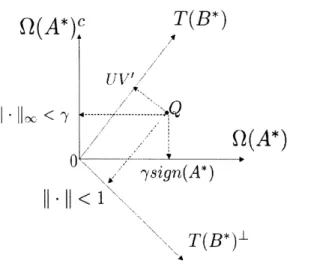
into "low-rank" and "sparse" parts may not exist; for example, the low-rank matrix may itself be very sparse leading to identifiability issues. In order to characterize when a unique decomposition is possible we develop a notion of rank-sparsity incoherence, an uncertainty principle between the sparsity pattern of a matrix and its row/column spaces. This condition is based on quantities involving the tangent spaces to the al-gebraic variety of sparse matrices and the alal-gebraic variety of low-rank matrices [79]. Another point of ambiguity in the problem statement is that one could subtract a nonzero entry from A* and add it to B*; the sparsity level of A* is strictly improved while the rank of B* is increased by at most 1. Therefore it is in general unclear what the "true" sparse and low-rank components are. We discuss this point in greater detail in Section 3.4.2 following the statement of the main theorem. In particular we describe how our identifiability and recovery results for the decomposition problem are to be interpreted.

Two natural identifiability problems may arise. The first one occurs if the low-rank matrix itself is very sparse. In order to avoid such a problem we impose certain conditions on the row/column spaces of the low-rank matrix. Specifically, for a matrix M let T(M) be the tangent space at M with respect to the variety of all matrices with rank less than or equal to rank(M). Operationally, T(M) is the span of all matrices with row-space contained in the row-space of M or with column-space contained in the column-space of M; see (3.7) for a formal characterization. Let ((M) be defined as

(31)

Sec. 3.1. Introduction

follows:

(M) A max ||NIloo. (3.1)

NET(M),

lINII<1

Here is the spectral norm (i.e., the largest singular value), and

||

denotes the largest entry in magnitude. Thus E(M) being small implies that (appropriately scaled) elements of the tangent space T(M) are "diffuse", i.e., these elements are not too sparse; as a result M cannot be very sparse. As shown in Proposition 3.4.3 (see Section 3.4.3) a low-rank matrix M with row/column spaces that are not closely aligned with the coordinate axes has small ((M).

The other identifiability problem may arise if the sparse matrix has all its support concentrated in one column; the entries in this column could negate the entries of the corresponding low-rank matrix, thus leaving the rank and the column space of the low-rank matrix unchanged. To avoid such a situation, we impose conditions on the sparsity pattern of the sparse matrix so that its support is not too concentrated in any row/column. For a matrix M let Q(M) be the tangent space at M with respect to the variety of all matrices with number of nonzero entries less than or equal to Isupport(M)

I.

The space Q(M) is simply the set of all matrices that have support contained within the support of M; see (3.5). Let p(M) be defined as follows:

[p(M)

A

max

||NI|.

(3.2)

NEQ(M), ||N||oo $

The quantity p(M) being small for a matrix implies that the spectrum of any element of the tangent space Q(M) is "diffuse", i.e., the singular values of these elements are not too large. We show in Proposition 3.4.2 (see Section 3.4.3) that a sparse matrix M with "bounded degree" (a small number of nonzeros per row/column) has small j(M).

For a given matrix M, it is impossible for both quantities ((M) and P(M) to be simultaneously small. Indeed, we prove that for any matrix M

#

0 we must have that

((M)pa(M) > 1 (see Theorem 3.3.1 in Section 3.3.3). Thus, this uncertainty principle asserts that there is no nonzero matrix M with all elements in T(M) being diffuse and all elements in Q(M) having diffuse spectra. As we describe later, the quantities ( and ya are also used to characterize fundamental identifiability in the decomposition problem.

In general solving the decomposition problem is intractable; this is due to the fact that it is intractable in general to compute the rigidity of a matrix (see Section 3.2.2), which can be viewed as a special case of the sparse-plus-low-rank decomposition

(32)

3'2 CHAPTER 3. RANK-SPARSITY UNCERTAINTY PRINCIPLES AND MATRIX DECOMPOSITION relaxations. We formulate a convex optimization problem for decomposition using a combination of the

E

₁norm and the nuclear norm. For any matrix M the fi norm is given by

||1

=

|MLAI,I

i~j

and the nuclear norm, which is the sum of the singular values, is given by ||Ml, = Zok(M),

k

where

{

0k(M)} are the singular values of M. The

e

1 norm has been used as an effective

surrogate for the number of nonzero entries of a vector, and a number of results pro-vide conditions under which this heuristic recovers sparse solutions to ill-posed inverse problems [29, 53,54]. More recently, the nuclear norm has been shown to be an effec-tive surrogate for the rank of a matrix [64]. This relaxation is a generalization of the previously studied trace-heuristic that was used to recover low-rank positive semidefi-nite matrices [108]. Indeed, several papers demonstrate that the nuclear norm heuristic recovers low-rank matrices in various rank minimization problems [30, 121]. Based on these results, we propose the following optimization formulation to recover A* and B* given C = A* + B*:

(AB)

=

arg min g||A||1 +

IIBfl,

A,B ₍₃₃₎

s.t. A + B = C.

Here -y is a parameter that provides a trade-off between the low-rank and sparse compo-nents. This optimization problem is convex, and can in fact be rewritten as a semidef-inite program (SDP) [139] (see Appendix A.1).

We prove that (A, B) = (A*, B*) is the unique optimum of (3.3) for a range of -y if pi(A*)((B*) < 1 (see Theorem 3.4.1 in Section 3.4.2). Thus, the conditions for exact

recovery of the sparse and low-rank components via the convex program (3.3) involve the tangent-space-based quantities defined in (3.1) and (3.2). Essentially these conditions specify that each element of Q(A*) must have a diffuse spectrum, and every element of T(B*) must be diffuse. In a sense that will be made precise later, the condition p(A*)((B*) < - required for the convex program (3.3) to provide exact recovery is slightly tighter than that required for fundamental identifiability in the decomposition problem. An important feature of our result is that it provides a simple deterministic condition for exact recovery. In addition, note that the conditions only depend on the

(33)

Sec. 3.1. Introduction 33

row/column spaces of the low-rank matrix B* and the support of the sparse matrix A*, and not the magnitudes of the nonzero singular values of B* or the nonzero entries of

A*. The reason for this is that the magnitudes of the nonzero entries of A* and the

nonzero singular values of B* play no role in the subgradient conditions with respect to the fi norm and the nuclear norm.

In the sequel we discuss concrete classes of sparse and low-rank matrices that have small y and ( respectively. We also show that when the sparse and low-rank matrices A* and B* are drawn from certain natural random ensembles, then the sufficient conditions of Theorem 3.4.1 are satisfied with high probability; consequently, (3.3) provides exact recovery with high probability for such matrices.

* 3.1.2 Previous work using incoherence

The concept of incoherence was studied in the context of recovering sparse represen-tations of vectors from a so-called "overcomplete dictionary"

[52].

More concretely consider a situation in which one is given a vector formed by a sparse linear combina-tion of a few elements from a combined time-frequency diccombina-tionary, i.e., a vector formed

by adding a few sinusoids and a few "spikes"; the goal is to recover the spikes and

sinusoids that compose the vector from the infinitely many possible solutions. Based on a notion of time-frequency incoherence, the fi heuristic was shown to succeed in recovering sparse solutions [51]. Incoherence is also a concept that is used in recent work under the title of compressed sensing, which aims to recover "low-dimensional" objects such as sparse vectors [29,54] and low-rank matrices [30,121] given incomplete observations. Our work is closer in spirit to that in [52], and can be viewed as a method to recover the "simplest explanation" of a matrix given an "overcomplete dictionary" of sparse and low-rank matrix atoms.

* 3.1.3 Outline

In Section 3.2 we elaborate on the applications mentioned previously, and discuss the implications of our results for each of these applications. Section 3.3 formally describes conditions for fundamental identifiability in the decomposition problem based on the quantities ( and y defined in (3.1) and (3.2). We also provide a proof of the rank-sparsity uncertainty principle of Theorem 3.3.1. We prove Theorem 3.4.1 in Section 3.4, and also provide concrete classes of sparse and low-rank matrices that satisfy the sufficient conditions of Theorem 3.4.1. Section 3.5 describes the results of simulations of our

(34)

34 CHAPTER 3. RANK-SPARSITY UNCERTAINTY PRINCIPLES AND MATRIX DECOMPOSITION approach applied to synthetic matrix decomposition problems. We conclude with a discussion in Section 3.6. Appendix A provides additional details and proofs.

* 3.2 Applications

In this section we describe several applications that involve decomposing a matrix into sparse and low-rank components.

* 3.2.1 Graphical modeling with latent variables

We begin with a problem in statistical model selection. In many applications large covariance matrices are approximated as low-rank matrices based on the assumption that a small number of latent factors explain most of the observed statistics (e.g., principal component analysis). Another well-studied class of models are those described

by graphical models [93] in which the inverse of the covariance matrix (also called the

precision or concentration or information matrix) is assumed to be sparse (typically this sparsity is with respect to some graph). Consequently, a natural sparse-plus-low-rank decomposition problem arises in latent-variable graphical model selection, which we discuss in more detail in Chapter 4.

N

3.2.2 Matrix rigidity

The rigidity of a matrix M, denoted by RM(k), is the smallest number of entries that need to be changed in order to reduce the rank of M below k. Obtaining bounds on rigidity has a number of implications in complexity theory [99], such as the trade-offs between size and depth in arithmetic circuits. However, computing the rigidity of a matrix is intractable in general [38, 101]. For any M e R"X' one can check that RM(k) _ (n - k)2 (this follows directly from a Schur complement argument). Generically every M E R", " is very rigid, i.e., RM(k) = (n- k)2 [138], although special

classes of matrices may be less rigid. We show that the SDP (3.3) can be used to compute rigidity for certain matrices with sufficiently small rigidity (see Section 3.4.4 for more details). Indeed, this convex program (3.3) also provides a certificate of the sparse and low-rank components that form such low-rigidity matrices; that is, the SDP

(3.3) not only enables us to compute the rigidity for certain matrices but additionally

(35)

Sec. 3.2. Applications 35

U 3.2.3 Composite system identification

A decomposition problem can also be posed in the system identification setting. Linear

time-invariant (LTI) systems can be represented by Hankel matrices, where the matrix represents the input-output relationship of the system [131]. Thus, a sparse Hankel matrix corresponds to an LTI system with a sparse impulse response. A low-rank Hankel matrix corresponds to a system with small model order, and provides a minimal realization for a system [65]. Given an LTI system H as follows

H = Hs + Hir,

where H, is sparse and Hir is low-rank, obtaining a simple description of H requires decomposing it into its simpler sparse and low-rank components. One can obtain these components by solving our rank-sparsity decomposition problem. Note that in practice one can impose in (3.3) the additional constraint that the sparse and low-rank matrices have Hankel structure.

* 3.2.4 Partially coherent decomposition in optical systems

We outline an optics application that is described in greater detail in [63]. Optical imaging systems are commonly modeled using the Hopkins integral [75], which gives the output intensity at a point as a function of the input transmission via a quadratic form. In many applications the operator in this quadratic form can be well-approximated by a (finite) positive semi-definite matrix. Optical systems described by a low-pass filter are called coherent imaging systems, and the corresponding system matrices have small rank. For systems that are not perfectly coherent various methods have been proposed to find an optimal coherent decomposition [115], and these essentially identify the best approximation of the system matrix by a matrix of lower rank. At the other end are incoherent optical systems that allow some high frequencies, and are characterized

by system matrices that are diagonal. As most real-world imaging systems are some

combination of coherent and incoherent, it was suggested in [63] that optical systems are better described by a sum of coherent and incoherent systems rather than by the best coherent (i.e., low-rank) approximation as in [115]. Thus, decomposing an imaging system into coherent and incoherent components involves splitting the optical system matrix into low-rank and diagonal components. Identifying these simpler components has important applications in tasks such as optical microlithography [75,115].

Convex optimization methods for graphs and statistical modeling

Convex Optimization Methods for

Graphs and Statistical Modeling

JUN 17 2011

LIBRARIES

ARCHIVES

o-visor

n)u~fr.

noumuejski

Convex Optimization Methods for

Graphs and Statistical Modeling

e

Acknowledgments

Contents

Chapter 1

Introduction

U

1.1 Main Contributions

Rank-Sparsity Uncertainty Principles and Matrix Decomposition

Latent Variable Gaussian Graphical Model Selection

Convex Optimization for Inverse Problems

Convex Graph Invariants

gi

Chapter 2

Background

[79]

* 2.1 Basics of Convex Analysis

E

function

f

at a point k in its domain by Of(k). The subdifferential

af(i)

consists of

f (x)

f (k) + (y,x

2.2 Representation of Convex Sets

M

2.2.1 Cross-polytope

BP

=

{x

E RP

|

lxii

<

I

+

{1,

Izil

2.2.2 Nuclear-norm ball

|| - | [82]:

|IX||,

= max{Tr(X'Y)I

IIYII

1}.

{X

{UM'+

{tUVT

IIWI|

2.2.3 Permutahedron

{

y

y

<Zxi, Vk=1,...,p-1,

and

Eyi=

Xi.

(2.2)

Qk(c)=

y E RP

y

C

}

{y

I

+

O(p

* 2.2.4 Schur-Horn orbitope

{N

E

_+l}P}.