Robust Multi-Objective Optimization in Aerodynamics using MGDA

HAL Id: hal-00919215

https://hal.inria.fr/hal-00919215

Submitted on 16 Dec 2013

HAL is a multi-disciplinary open access

archive for the deposit and dissemination of

sci-entific research documents, whether they are

pub-lished or not. The documents may come from

teaching and research institutions in France or

abroad, or from public or private research centers.

L’archive ouverte pluridisciplinaire HAL, est

destinée au dépôt et à la diffusion de documents

scientifiques de niveau recherche, publiés ou non,

émanant des établissements d’enseignement et de

recherche français ou étrangers, des laboratoires

publics ou privés.

Robust Multi-Objective Optimization in Aerodynamics

using MGDA

Daigo Maruyama

To cite this version:

Daigo Maruyama. Robust Multi-Objective Optimization in Aerodynamics using MGDA. [Research

Report] RR-8428, INRIA. 2013. �hal-00919215�

Robust Multi-Objective Optimization in

Aerodynamics using MGDA

Daigo Maruyama

N° 8428         December 2013    

S

N

0249

-6399

Robust Multi-Objective Optimization in Aerodynamics using MGDA

Daigo Maruyama

1

Project-Team OPALE

Research Report

 N° 8428

—

December 2013

— 20 pages.

 

Abstract:  This study deals with robust design optimization strategies in aerodynamics, by considering geometric parameters as  uncertainty factors, with application to transonic airfoil design. Mean and standard deviation of the aerodynamic coefficients are  considered  as  cost  functions  for  a  multi‐objective  optimization  problem.  Statistical  moments  are  evaluated  using  Monte‐Carlo  simulations (MCS), on the basis of Radial Basis Functions (RBF) surrogate models. The multi‐objective optimization is achieved  using the Multiple‐Gradient Descent Algorithm (MGDA), which permits to find a descent direction for all criteria simultaneously,  starting from a set of initial design points.  The airfoil shape parameterization is carried out using the PARSEC approach to define  significant  design  parameters.  Moreover,  the  ANOVA  (ANalysis  Of  Variance)  technique  is  used  to  identify  the  most  relevant  parameters  for  aerodynamic  criteria.  The  proposed  approach  is  illustrated  on  a  practical  robust  design  problem  involving  four  statistical cost functions. 

 

Key‐words: Robust design optimization, parameterization, surrogate models, Multi‐gradient descent algorithm   

Robust Multi-Objective Optimization in Aerodynamics using MGDA

Résumé  :  Cette  étude  concerne  les  stratégies  d’optimisation  robuste  en  aérodynamique,  en  considérant  des  paramètres  géométriques comme variables aléatoires, avec application à la conception de profils transsoniques. La moyenne et l’écart‐ type  des  coefficients  aérodynamiques  sont  considérés  comme  des  fonctions  de  coûts  pour  un  problème  d’optimisation  multiobjectif.  Les  moments  statistiques  sont  évalués  par  simulations  de  Monte‐Carlo  (MCS),  sur  la  base  de  modèles  approchés de type fonctions à bases radiales. L’optimisation multiobjective est réalisée à l’aide de l’algorithme de descente  à gradient multiple, qui permet de trouver une direction de descente pour tous les critères simultanément, à partir d’un  ensemble de points de conception initiaux. La paramétrisation de la forme des profils est effectuée par l’approche PARSEC  pour  définir  des  paramètres  de  conception  ayant  une  signification  pour  l’aérodynamique.  De  plus,  la  technique  ANOVA  (analyse de la variance) est utilisée pour identifier les paramètres les plus importants pour les critères aérodynamiques.  L’approche proposée est illustrée pour un problème pratique de conception robuste impliquant quatre fonctions de coûts  statistiques. 

   

1. Introduction ... 6

2. Problem statement ... 6

3. Methods ... 8

3.1 Definition of geometric parameters as both design variables and uncertainty factors ... 8

3.2 Surrogate models for statistical moments estimation and MGDA ... 9

3.3 ANOVA technique ... 10

4. Application to aerodynamic design of transonic airfoils ... 11

4.1 Classical optimization ... 11

4.2 Robust optimization ... 13

Conclusion ... 19

6   

   Daigo Maruyama  

Inria

1. Introduction

In the last decades, Computational Fluid Dynamics (CFD) has known a significant development and is now used for practical aerodynamic shape optimization. The optimization methodologies have also matured with the industrial context and Multidisciplinary Design Optimization (MDO) is now widely used and essential in the aerospace field. Presently, a major issue is robust design, for which uncertainties are taken into account during the design phase.

There are various approaches in aerodynamic shape optimization, which are based on different points of view. Usually in aerodynamic shape design, optimum design parameters are determined to minimize or maximize cost functions. In this classical deterministic approach, the optimized solutions would cause performance losses due to uncertainty factors such as manufacturing tolerance, neglected details, structural deformation, icing, as well as operational parameters. There is another viewpoint, for which stability of cost functions with respect to design variables or operational parameters is also important while optimizing the cost functions. Robust design mentioned above aims at considering off-design conditions as fluctuations of operational parameters [1-4].

The objective of this study is to take into account the uncertainty related to geometrical variables during the design optimization procedure. Therefore, design variables are regarded as uncertainty factors at the same time. In this report, uncertainty analysis and robust optimization applied to aerodynamic airfoil design in transonic flow are presented. Stochastic models are introduced to quantify the impact of uncertainty factors on aerodynamic coefficients. The parameterization of airfoil geometries, which is related to quantifications of uncertainty factors, is also an important issue. Many parameterization methods have been proposed so far, such as NURBS using control points, CST [5], PARSEC [6], etc. To consider manufacturing process, NURBS using control points would be more practical. However, to investigate uncertainty factors from aerodynamic viewpoint, PARSEC technique is preferred since the related design parameters have a significant role for aerodynamic performance.

2. Problem statement

A general description of the problem is provided in this section. To be as general as possible, we make the assumption that uncertainty arises from geometrical design variables

x

_{as well as operational variables}

a

_{. Thus, we consider the design}

variables and operational variables as random variables _X and A, characterized by two uncorrelated probability density functions

f

X and

f

A defined over

Ω

_X and

Ω

_A. For the sake of simplicity, we assume that A is perfectly known and X is Gaussian with mean

µ

_X, which will be adjusted during the optimization, and fixed standard deviation (Std)

σ

_X.

In a statistical framework, we intend to solve the design problem by accounting for statistical moments of the cost functional, such as the expectation

µ

j and the Std

σ

j:

µ

_j

= E j x, a

!"

₍

₎

#$=

j x, a

(

)

f

_X

_{( )}

_x

f

_A

_{( )}

a

_{d x da}

ΩA

∫

ΩX

∫

σ

_j

=

E ( j x, a

(

)

− µ

j

)

2

!"

#$ =

(

j x, a

(

)

− µ

j

)

2

f

X

( )

x

f

A

( )

a

d x da

Ω_A

∫

Ω_X

∫

(1)

A typical multi-criterion strategy would consist in minimizing mean and Std, with respect to

x

_:

Minimize

_µ

j

( )

x

Minimize

σ

_j

_{( )}

_x

(2)

Thus, the robust counterpart of a classical optimization with a cost function j, is the multi-objective optimization with two cost functions

µ

j and

σ

j. The estimation of statistical moments (1) and (2) are presented in Section 3.2.

To solve the multi-objective optimization problem, the Multiple-Gradient Descent Algorithm (MGDA) developed in Opale Project-Team [7] is employed. Details on the underlying theory of MGDA can be found in [7]. Some practical details to obtain the Pareto front solutions and some applications are presented in [8]. Basically, MGDA is an extension of the classical steepest-descent method in case of several criteria. It consists in combining the descent directions related to the different cost

functions to define a direction, which improves all criteria simultaneously. Here, we just mention two key elements of MGDA: the calculation of the search direction and the step length.

1. The search direction vector is determined by

- Explicit geometric features when only two cost functions are considered [7, 8]

- Gram-Schmidt Orthogonalization of the gradient vector set when the number of cost function is more than two [9]

2. The step length is determined by the golden section method.

Note that the use of Gram-Schmidt Orthogonalization requires a number of objective functions lower than that of design variables.

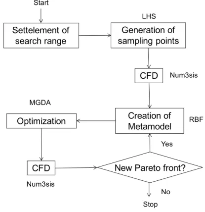
The approach used for uncertainty qualification and the strategy proposed for robust design are described herein. First of all, we define the search domain for the design variables, which will also impact the evaluation of the statistical moments of the cost functions, as explained later. Then, initial sampling points are determined by Latin Hypercube Sampling (LHS) in the selected search domain. The aerodynamic coefficients Cl and Cd are obtained by CFD calculations using the Num3sis platform, which is developed in OPALE team [10]. In classical optimization cases, these aerodynamic coefficients are considered directly as the cost functions. Alternatively, in robust optimization cases, the mean and Std of each aerodynamic coefficient are considered as objective functions. In this study, for the sake of simplicity, design variables only are considered as uncertain factors. Thus, uncertainty related to operational conditions is not addressed here. As first step to investigate geometric uncertainty factors from aerodynamic viewpoints, the design variables are represented by PARSEC parameterization [6]. Then, surrogate models are constructed for each cost function to estimate the statistical moments. Before solving the optimization problem, the contributions of each design variable to the statistical moments of the cost functions are quantified by ANOVA (ANalysis Of VAriance). The motivation to use ANOVA is to determine if some design variables are negligible and to select a relevant design space. The details on the application of ANOVA are described later. Flow charts of classical optimization and robust optimization are shown in Figures 1 and 2, respectively. Details on each method in the flow charts are presented in the next section. Firstly, initial sampling points

x

are generated by LHS. The parameterization of airfoils as design variables is conducted by PARSEC. CFD calculations are carried out to obtain aerodynamic coefficients. Then, a response surface is constructed for each cost function to lead the optimization process. Then, for the classical optimization, MGDA is used to update the design parameters and new cost function values for each new point are obtained by CFD calculations. This process is iterated until convergence to their Pareto front.

FIGURE 1: Flow chart of classical optimization

Generation of

sampling points

CFD

Creation of

Metamodel

Optimization

New Pareto front?

CFD

LHS Num3sis RBF MGDA Num3sis Yes No Stop Start

Settelement of

search range

8   

   Daigo Maruyama  

Inria In the robust optimization process, two steps are added, compared to the classical optimization process. First, the statistical moments of the aerodynamic coefficients are calculated by MCS on the basis of surrogate models. Second, ANOVA is introduced for a possible reconsideration of the design space and modification of the search range.

FIGURE 2: Flow chart of robust optimization

3. Methods

3.1 Definition of geometric parameters as both design variables and uncertainty factors

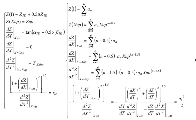
For the purpose of working with aerodynamically significant geometric features, we used the PARSEC method [6]. PARSEC is one of the conventional parameterizations for transonic airfoils to control the local shock wave on the upper surface. It has been applied to aerodynamic shape optimization problems [11-14]. It has been modified to capture the suction peak at the leading edge in transonic flow or in supersonic flow [13,14]. In this framework, the shapes of two-dimensional transonic airfoils are controlled by 11 parameters and are described by the following polynomial terms.

∑

= −

=

6 1 5 . 0 n n n

X

a

Z

₍₃₎

Figure 3 depicts these 11 parameters.

Z

UP,

Z

LO and

X

UP,

X

LO represent the maximum thickness and their positions in

the chord direction, respectively.

Z

XXUP and

Z

XXLO are curvatures at the maximum thickness positions.

r

is a radius, which

represents the curvature at the leading edge.

_Z

_TE and

Δ

_Z

_TE are the position of the trailing edge and its thickness, respectively.

α

_TE and

β

_TE are the angle representations of the camber and thickness at the trailing edge, respectively. These 11 parameters are considered as aerodynamically significant ones in transonic airfoil design. The coefficients

(

n

=

1 !

,

,

6

)

a

n in Eq. (3) are uniquely determined by solving the following six-equation system obtained by geometric

considerations:

Generation of

sampling points

CFD

Creation of

Metamodel

Optimization of

stochastic parameters

New Pareto front?

CFD

LHS Num3sis RBF MGDA Num3sis Yes No Stop Start

Settelement of

search range

ANOVA

- Creation of new search range

- Selection of significant design variables

Yes

(

)

                      =                 + − = = × − = = Δ + = = = = = = le X X XXup Xup X Xup X TE TE X TE TE r dX Z d dX dZ Z dX Z d dX dZ dX dZ Zup Xup Z Z Z Z 0 2 2 5 . 1 2 0 2 2 1 1 0 5 . 0 tan ) ( 5 . 0 ) 1 (

β

α

( )

(

)

(

)

(

)

( )

(

) (

)

( )                           = −               +       − =                 + − ⋅ − ⋅ − = ⋅ − = ⋅ − = = = = = = = = − = − = = = = = − =

∑

∑

∑

∑

∑

2 1 5 . 0 5 . 1 5 . 0 5 . 0 1 2 1 0 2 2 0 2 2 5 . 1 2 2 0 2 2 5 . 1 2 0 6 1 5 . 2 2 2 5 . 1 6 1 6 1 1 6 1 5 . 0 6 1 a dT X d dT dZ dT Z d dT dX dT dZ dT dX dX Z d dX dZ Xup a n n dX Z d Xup a n dX dZ a n dX dZ Xup a Xup Z a Z T T X X n n n Xup X n n n Xup X n n X n n n n n (4)

Then, the airfoil coordinates are determined by Eq. (3), for arbitrary X (

0

_{≤ X}

≤

1

). The most significant design variables for aerodynamic coefficients will be quantified by using ANOVA, shown in Section 3.3.

FIGURE 3: Description of PARSEC geometric parameters

3.2 Surrogate models for statistical moments estimation and MGDA

In order to have a reasonable computational cost, the mean and Std of cost functions are estimated using response surfaces (also called surrogate models), which are constructed using Radial Basis Functions (RBFs). The surrogate model

f

( )

_x

, at arbitrary design variables

_x

, is represented by the following equation:

( )

( )

_∑

= Τ

=

=

m i i i

g

f

1

β

x

g

β

x

, where

g

i

=

φ

(

r

i

( )

x

)

(5)

Here, β is a vector uniquely determined for a given cost function and set of the sampling points. m is the number of sampling points,

φ

is a radial basis function, determined by the Euclidean distance between

_x

and the sampling point. Details on the determination of β can be found in [15]. Here, we used Gaussian radial basis function:

φ

=

exp

( )

−

r

2 .

10       Daigo Maruyama   Inria

( )

₍

_{( )}

₎

∑

= Τ

∂

∂

=

∂

∂

=

∂

∂

m i i i i

r

r

f

1

'

x

x

x

g

β

x

x

φ

β

, where

(

)

( )

x

x

x

x

i i i

r

r

₋

Τ

=

∂

∂

(6)

A more detailed discussion on gradient and Hessian of surrogated models based on RBF can be found in [15].

Mean and Std of the cost functions are evaluated by using the constructed surrogate models. According to Eq. (1), the mean f

µ

and Std

σ

_f could be evaluated by numerical integration. For example, the integral of Eq. (5) is represented as:

( )

x

d

x

(

r

( )

x

)

d

x

f

m i i i

∑ ∫

∫

=

=

1

φ

β

(7)

A difficulty arises when the number of parameters is large, since this integral is defined in a space of high-dimension. To reduce the computational cost, two possibilities could be envisaged:

1. Use of Monte Carlo Simulation (MCS), whose accuracy does not depend on the dimension 2. Reduce the number of design variables and use classical numerical integration rules

The first approach is based on random numbers yielding a noisy estimation of statistical moments. Thus, there is a possibility that MGDA converges to a local minimum. The second approach requires defining a selection of dominant design variables, which is also related to ANOVA, described in the next section. In this report, we present results obtained by using MCS to estimate the statistical moments. Therefore, the mean

µ

_f and Std

σ

_f are estimated by random sampling points xi as follows:

( )

∑

=

=

N i i f

f

N

₁

1

x

µ

(8)

( )

(

)

∑

=

−

−

=

N i f i f

f

N

₁ 2

1

1

_µ

σ

_x

(9)

where N is the number of the sampling points xi. The sampling points are determined using a random number generator. To generate a Gaussian distribution, we employ the Box-Muller algorithm to transform a uniform distribution. Finally, the evaluated mean

µ

_f and Std

σ

_f are dependent on the following three factors:

- The selected design space

- The statistical moments of design variables

- The number of the random sampling points used in MCS

To select a relevant design space, ANOVA is used and described in the next section.

3.3 ANOVA technique

ANOVA is used to quantify the influence of design variables to each cost function [16]. First of all, we calculate the total mean and total variance for a cost function

F

(

x

1

,

!

,

x

n

)

:

µ

total

=

∫

!

∫

F x

(

1

,!, x

n

)

dx

1

!dx

n (10)

(

)

[

]

∫ ∫

− = n total n total ! F x ! x dx1!dx 2 1 2 _{, ,}

µ

σ

(11)

To evaluated the effect of an arbitrary design variable xi to the objective function, the partial mean and variance of the design variable xi are evaluated by the following equations:

σ

2

_x

i

( )

=

!"

µ

i

( )

x

i

#$

2

dx

_i

∫

(13)

Finally, the effect of the design variable xi to the objective function

F

(

x

1

,

!

,

x

n

)

is considered to be:

( )

2 2 total i x

σ

σ

(14)

Thus, this technique permits to quantify the influence of the design variables, for each objective function. In practical use, ANOVA is applied to surrogate models, the integrals in Eqs. (10) - (12) being evaluated by MCS.

4. Application to aerodynamic design of transonic airfoils

In this section, we present the application of the proposed method to transonic airfoil design. All of the CFD calculations used to evaluate aerodynamic coefficients are inviscid analyses based on two-dimensional compressible Euler equations. The grids are generated using the Gmsh software, for each new configuration. The Mach number and angle of attack as operational parameters are fixed to 0.8 and 4 degrees, respectively. For these conditions, airfoils are expected to generate strong shock waves from their leading edges.

4.1 Classical optimization

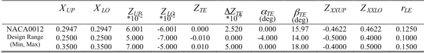
At first, some classical design optimization cases are briefly introduced. The objective functions are the lift coefficient Cl and drag coefficient Cd. The design variables are the 11 PARSEC parameters shown in Fig. 3. Based on the NACA0012 airfoil as baseline, the search range is set as shown in Table 1. Thus, the following multi-criterion shape optimization problem is:

( )

( )

x

x

d l

C

Minimize

C

Maximize

_x

∈

_R

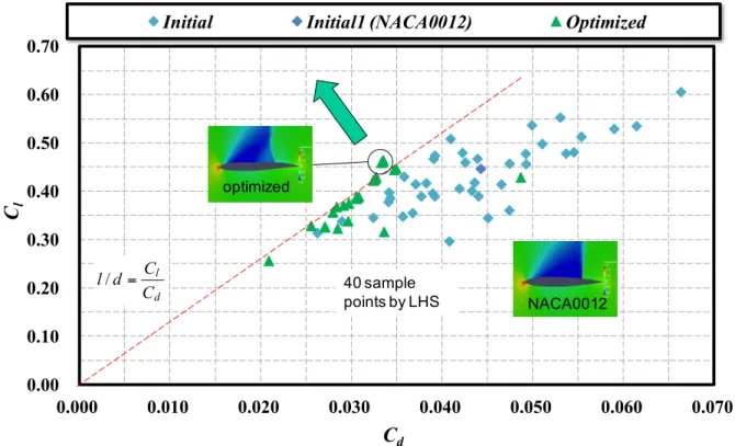
11 (15)

In the design space, 40 sampling points are generated randomly by LHS. Figure 4 shows Cl-Cd distribution for this initial sampling, for optimized designs obtained after three iterations of the cycle shown in Fig. 1, and for baseline NACA0012 for comparison. It can be observed that most of the initial points converge to the higher lift-to-drag ratio (Cl/Cd) line, indicated in red. The pressure fields for the airfoil with the highest lift-to-drag ratio and for NACA0012 airfoil are also shown in the figure. As reference, ANOVA results obtained from the surrogate models based on the CFD calculations are presented in Fig. 5. It is confirmed that the camber and thickness effects at the trailing edge, represented by

α

,

β

and the curvature of the upper surface

Z

XXUP, are the most significant variables for both aerodynamic coefficients. These parameters control the shape at

the trailing edge, which influences aerodynamic performance much in transonic flow, and the shape of the suction surface, which influences the shock wave generated. In fact the optimized airfoil, shown in Fig. 4, underlines the significance of these three parameters. In particular, it can be seen that the generated shock wave is controlled by the curvature of the upper element

Z

XXUP.

Table 1: PARSEC parameters for classical optimization.

UP

X

X

_LO UP

Z

*10-2 LO

Z

*10-2 TE

Z

TE

Z

Δ

*10-3 (deg)

α

TE (deg)

β

TE XXUP

Z

Z

_XXLO

_r

_LE NACA0012 0.2947 0.2947 6.001 -6.001 0.000 2.520 0.000 15.97 -0.4622 0.4622 0.1250 Design Range (Min, Max) 0.2500 _0.3500 0.2500 _0.3500 5.000 _7.000 -7.000 _-5.000 -0.010 _0.010 0.000 _5.000 -4.000 _0.000 14.00 _18.00 -0.5000 _-0.4000 0.4000 _0.5000 0.1000 _0.1500

12   

   Daigo Maruyama  

Inria FIGURE 4: Cl - Cd distributions for classical optimization

l

C

C

_d

FIGURE 5: ANOVA result for classical optimization

0.00

0.10

0.20

0.30

0.40

0.50

0.60

0.70

0.000

0.010

0.020

0.030

0.040

0.050

0.060

0.070

C

l

C

_d

Initial

Initial1 (NACA0012)

Optimized

d l C C d l/ _{= 40 sample} points by LHS optimized NACA0012

Xup Xlo Zup

Zlo Zte_ΔZte

α β Zxxup Zxxlo r Xup Xlo Zup Zlo Zte ΔZte α β Zxxup Zxxlo r

Xup Xlo Zup

Zlo ZteΔZte

α β Zxxup Zxxlo r Xup Xlo Zup Zlo Zte ΔZte α β Zxxup Zxxlo r

4.2 Robust optimization

As explained in Section 2, robust optimization is treated as multi-objective optimization of statistical moments of the cost functions. Note that in this context, the design variables are considered as uncertainty factors at the same time. Therefore, we put an additional step to the classical optimization process. We reconsider the design space using ANOVA, after CFD calculations of randomly selected sampling points. This step is intended for:

- Neglecting low-influence parameters - Generating new parameter ranges

This strategy "feedback of settlement of search range" is shown in Fig. 2. In this study, the following three robust optimization cases are finally discussed: 1. Robust optimization with initial design space (named "Initial")

2. Robust optimization by neglecting low-influence parameters using ANOVA (named "Selected") 3. Robust optimization with new parameter ranges using ANOVA (named "Range")

In these three cases, the cost functions are the mean and Std of Cl (

µ

Cl,

σ

Cl) and Cd (

µ

Cd,

σ

Cd) calculated by Eqs. (8)

and (9). The number and the range of the design variables are dependent on the cases. In robust optimization, the aim is to take into account design fluctuations and to investigate their effects on aerodynamics. Based on the baseline NACA0012 airfoil, the search range is defined in Table 2. As for the classical optimization, the Mach number and angle of attack are fixed to 0.8 and 4 degrees, respectively. 40 sampling points are randomly generated by LHS in the selected design space. The results obtained for these three cases are discussed in the following sections. Then, a summary of the contributions of these three cases to robust optimization design is described.

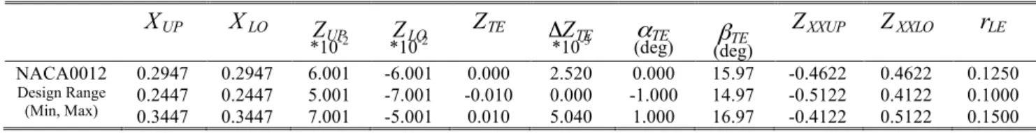
Table 2. Initial PARSEC parameters for robust optimization.

UP

X

X

_LO UP

Z

*10-2 LO

Z

*10-2 TE

Z

TE

Z

Δ

*10-3 (deg)

α

TE (deg)

β

TE XXUP

Z

Z

_XXLO

_r

_LE NACA0012 0.2947 0.2947 6.001 -6.001 0.000 2.520 0.000 15.97 -0.4622 0.4622 0.1250 Design Range (Min, Max) 0.2447 _0.3447 0.2447 _0.3447 5.001 _7.001 -7.001 _-5.001 -0.010 _0.010 0.000 _5.040 -1.000 _1.000 14.97 _16.97 -0.5122 _-0.4122 0.4122 _0.5122 0.1000 _0.1500

4.2.1 Robust optimization with initial design space

Robust optimization is firstly conducted in the initial design space defined in Table 2. The following multi-objective optimization problem is solved:

( )

( )

( )

( )

x

x

x

x

d l d l C C C C

Minimize

Minimize

Minimize

Maximize

σ

σ

µ

µ

x

∈

_R

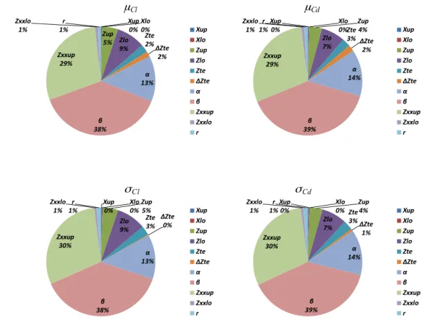
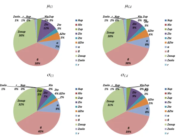
11 (16)

ANOVA results are obtained from the CFD simulations at the sampling points. Figure 6 shows the resulting analyses for the 4 objective functions. The characteristics of these 4 cost functions are similar to each other. It can be easily observed that the parameters

α

and

β

, which are related to the geometry at the trailing edge, and

Z

XXUP, the curvature of the upper surface,

are the most significant variables, like in the case of the classical optimization in the previous section. Two parameters related to the airfoil thickness

Z

UP and

Z

LO follow them. Regarding the other parameters, the influence of the thickness of the

trailing edge

Δ

_Z

_TE is much lower for Std of the aerodynamic coefficients.

These ANOVA results are helpful for uncertainty quantifications. As presented in Section 2, we use the ANOVA results to reconsider the design space. These modifications are detailed in the following sections.

14       Daigo Maruyama   Inria Cl

µ

µ

Cd Cl

σ

σ

Cd

FIGURE 6: ANOVA results for initial design space in robust optimization

4.2.2 Robust optimization by dominant design variables

One possible strategy to extract dominant parameters is to consider if the percentage of each design parameter is greater than that of the equally divided value (around 9% for 11 parameters). The three design parameters

α

,

β

and

Z

XXUP are selected

using this strategy. In this study, we choose to select the top 5 dominant parameters, according to Fig. 6 (

α

,

β

,

Z

XXUP, UP

Z

_and

Z

_LO ) because using MGDA the number of design variables must be greater than the number of objective functions. New sampling points are generated by LHS and CFD calculations are carried out to obtain new ANOVA results. The other 6 parameters are fixed to their respective baseline value. Therefore, the multi-objective optimization problem is changed as follows:

( )

( )

( )

( )

x

x

x

x

d l d l C C C C

Minimize

Minimize

Minimize

Maximize

σ

σ

µ

µ

x

∈

_R

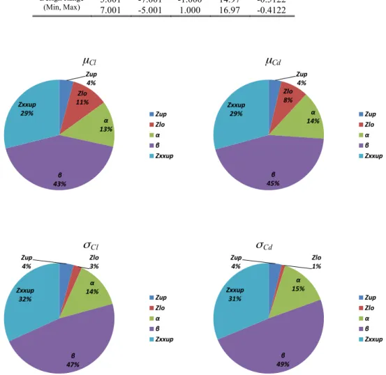
5 (17)

Table 3 shows the 5 selected design variables and their respective design ranges (the same as the initial ones). Figure 7 presents the analyses of ANOVA results for the 4 objective functions with respect to the newly selected design variables. It can be observed that the contributions of the parameters are different from previously. For instance, the contributions of

β

to

Xup 0% Xlo 0% Zup 5% Zlo 9% Zte 2% ΔZte 2% α 13% β 38% Zxxup 29% Zxxlo 1% r 1% Xup Xlo Zup Zlo Zte ΔZte α β Zxxup Zxxlo r Xup 0% Xlo 0% Zup 4% Zlo 7% Zte 3% ΔZte 2% α 14% β 39% Zxxup 29% Zxxlo 1% r 1% Xup Xlo Zup Zlo Zte ΔZte α β Zxxup Zxxlo r Xup 0% Xlo 0% Zup 5% Zlo 9% Zte 3% ΔZte 0% α 13% β 38% Zxxup 30% Zxxlo 1% r 1% Xup Xlo Zup Zlo Zte ΔZte α β Zxxup Zxxlo r Xup 0% Xlo 0% Zup 4% Zlo 7% Zte 3%_ΔZte 1% α 14% β 39% Zxxup 30% Zxxlo 1% r 1% Xup Xlo Zup Zlo Zte ΔZte α β Zxxup Zxxlo r

Std of both coefficients is greater than those to the mean. On the other hand, the characteristics of

Z

LO indicate the opposite

modification, especially for Std of Cd.

Table 3. Selected dominant PARSEC parameters for robust optimization.

UP

Z

*10-2 LO

Z

*10-2 (deg)

α

TE (deg)

β

TE XXUP

Z

NACA0012 6.001 -6.001 0.000 15.97 -0.4622 Design Range (Min, Max) 5.001 _7.001 -7.001 _-5.001 -1.000 _1.000 14.97 _16.97 -0.5122 _-0.4122 Cl

µ

µ

Cd Cl

σ

σ

Cd

FIGURE 7: ANOVA results for selected 5 dominant design variables in robust optimization

4.2.3 Robust optimization by new ranges of design variables

The previous studies have underlined the fact that a very small amount of design variables, in the context of PARSEC parameterization, have a very strong impact on the aerodynamic coefficient variations, and their moments if geometrical uncertainties are considered.

For this reason, we consider now a modification of the variable ranges. More precisely, the design variables, which have the most significant weight according to a first ANOVA study, will see their range decrease. For example, it can be observed by the ANOVA results using the initial design space, shown in Fig. 6, that the curvature of the upper surface

Z

XXUP has much

more influence to the aerodynamic performance than the lower surface

Z

XXLO. Therefore, we selected new design ranges for

the parameters whose percentages are greater than the percentage corresponding to the equally divided weight (around 9%). Using this approach, the three parameters

α

,

β

and

Z

XXUP are selected. The ranges of these three parameters have to be

Zup 4% Zlo 11% α 13% β 43% Zxxup 29% Zup Zlo α β Zxxup Zup 4% Zlo 8% α 14% β 45% Zxxup 29% Zup Zlo α β Zxxup Zup 4% Zlo 3% α 14% β 47% Zxxup 32% Zup Zlo α β Zxxup Zup 4% Zlo 1% α 15% β 49% Zxxup 31% Zup Zlo α β Zxxup

16   

   Daigo Maruyama  

Inria smaller than the initial ranges. The ranges of

α

,

β

and

Z

XXUP are chosen to be a quarter, a quarter and a half, according to

the occupation of the percentages in Fig. 6, respectively. The new parameter ranges are shown in Table 4. The multi-objective optimization problem considered is the same as the first case:

( )

( )

( )

( )

x

x

x

x

d l d l C C C C

Minimize

Minimize

Minimize

Maximize

σ

σ

µ

µ

x

∈

_R

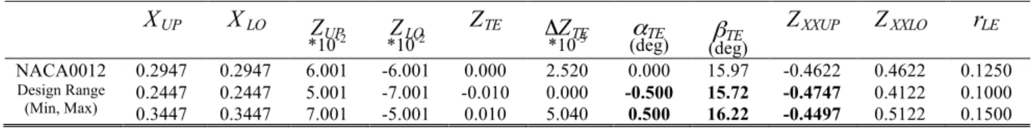
11 (18)

Only the parameter ranges are different from those of the first case shown in Table 2. Figure 8 represents the ANOVA results. The dominant parameters

β

and

Z

XXUP are not changed in the ratio. However, the other minor parameters have a weight

closer to the equally divided ratio (around 9%). The parameter

α

, which is one of the most dominant three parameters in the first case, is now at the same level as the other parameters.

Compared with the results of the 1st case, it can be mentioned that the two parameters

β

and

Z

XXUP have still a very

strong influence on the statistical moments of aerodynamic coefficients (mean and Std), even when the range of these parameters are small. This indicates that we have to pay much attention to uncertainty related to these two parameters, and that these parameters would make robust design problem more difficult.

Table 4. PARSEC parameters by new ranges for robust optimization.

UP

X

X

_LO UP

Z

*10-2 LO

Z

*10-2 TE

Z

_Δ

_Z

_TE *10-3 (deg)

α

TE (deg)

β

TE XXUP

Z

Z

_XXLO

_r

_LE NACA0012 0.2947 0.2947 6.001 -6.001 0.000 2.520 0.000 15.97 -0.4622 0.4622 0.1250 Design Range (Min, Max) 0.2447 _0.3447 0.2447 _0.3447 5.001 _7.001 -7.001 _-5.001 -0.010 _0.010 0.000 _5.040 -0.500 _0.500 15.72 _16.22 -0.4747 _-0.4497 0.4122 _0.5122 0.1000 _0.1500

Cl

µ

µ

Cd

Cl

σ

σ

Cd

FIGURE 8: ANOVA results for new ranges of design variables in robust optimization

4.2.4 Comparison of robust design optimization results

Finally, the results obtained by these three design exercises are discussed. The comparison of the case1 (Initial) to the case2 (Selected) and case3 (Range) focuses on two points. Firstly, we estimate the effect of the strategy of selecting dominant parameters. Then, we quantify the influence of aerodynamically significant parameters as uncertainty factors.

Figure 9 shows the distribution of the solution with respect to the three dominant parameters

α

,

β

and

Z

XXUP , selected by

the ANOVA technique for the original design space (Initial), after three iterations of the design cycle. One observes that the distribution of the solutions is different for the three cases (Initial, Selected and Range). Moreover, there is a cluster of design points for each case, except for "Selected" case. By taking into account the characteristics of the results of classical optimization case, presented in Section 4.1, we regard these clusters of design points as the Pareto solutions in robust optimization cases (even though we evaluate design parameters not cost functions here). Concerning the results of "Selected" case, it is difficult to find the Pareto front compared with other cases. Here we discuss mainly the results of "Initial" and "Range" cases. Some comments about "Selected" case are added later, based on the results of "Initial" and "Range" cases. The characteristics of the parameters obtained are different in "Initial" and "Range" cases, except for

α

. The parameter

α

, which represents the camber line at the trailing edge, is optimized to around the value 0.5 in both design spaces. The parameters

β

and

Z

XXUP, which are related to the thickness of the trailing edge and the curvature of the upper surface, have

different characteristics for the two cases “Initial” and “Range”. For "Initial" case, the airfoil is changed to have more thickness and sharper concavity, respectively. On the other hand, the change of these two parameters is moderate for "Range" case.

Figure 10 shows some configurations found, and the associated pressure fields. The airfoil configuration for "Selected" case has not only a different shape, but also has different aerodynamic coefficients from that of "Initial" case, which underlines the fact that the search is carried out in two different design spaces. The aerodynamic coefficients at the design point are not always better than the initial airfoil (NACA0012). However, we emphasize that these airfoils were designed by accounting for mean and Std of the aerodynamic coefficients. The difference between "Initial" and "Range" cases is the degree of robustness of design parameters. The results obtained by "Range" case are more robust with respect to fluctuations of the geometric

Xup 0% Xlo 0% Zup 3% Zlo 12% Zte 3% ΔZte 5% α 7% β 38% Zxxup 30% Zxxlo 1% r 1% Xup Xlo Zup Zlo Zte ΔZte α β Zxxup Zxxlo r Xup 0% Xlo 0% Zup 3% Zlo 9% Zte 3% ΔZte 6% α 8% β 38% Zxxup 30% Zxxlo 1% r 2% Xup Xlo Zup Zlo Zte ΔZte α β Zxxup Zxxlo r Xup 0% Xlo 0% Zup 5% Zlo 7% Zte 4% ΔZte 2% α 9% β 40% Zxxup 32% Zxxlo 1% r 0% Xup Xlo Zup Zlo Zte ΔZte α β Zxxup Zxxlo r Xup 0% Xlo 0% Zup 3% Zlo 9% Zte 3% ΔZte 5% α 8% β 39% Zxxup 31% Zxxlo 1% r 1% Xup Xlo Zup Zlo Zte ΔZte α β Zxxup Zxxlo r

18   

   Daigo Maruyama  

Inria parameters, because the ranges of the dominant parameters are limited. Concerning the "Selected" case, it is difficult to extract the information about the Pareto front.

In practical applications, geometric uncertainties, for instance in manufacturing process, may not occur according to the PARSEC parameters. As mentioned in the introduction, we use PARSEC parameterization to account for aerodynamic knowledge and make the design process more efficient. For example, the curvature of the upper element is much more significant than that of the lower one. This fact does not change even when the design search area of the upper element becomes smaller, as indicated in the results. The results obtained in this study could be employed for more realistic robust design applications, by using parameterization methods based on manufacturing parameters.

FIGURE 9: Distribution of three dominant design parameters (the square indicates the new design ranges for "Range". the circle indicates a cluster of design points)

FIGURE 10: Pressure distributions, (a) NACA0012, (b) Optimized using initial design space (Initial), (c) Optimized using selected design parameter (Selected), (d) Optimized using new design range (Range)

15.0 15.5 16.0 16.5 17.0 -1.5 -1.0 -0.5 0.0 0.5 1.0 1.5 β α

Initial Selected Range NACA0012

-0.50 -0.48 -0.46 -0.44 -0.42 -0.40 15.0 15.5 16.0 16.5 17.0 ZXX UP β

Initial Selected Range NACA0012

-1.5 -1.0 -0.5 0.0 0.5 1.0 1.5 -0.50 -0.48 -0.46 -0.44 -0.42 -0.40 α ZXXUP

Initial Selected Range NACA0012

Cl = 0.447 Cd = 0.0442 l/d = 10.10 Cl = 0.394 Cd = 0.0412 l/d = 9.54 Cl = 0.334 Cd = 0.0368 l/d = 9.09 Cl = 0.300 Cd = 0.0338 l/d = 8.73 (a) (b) (c) (d)

Conclusion

To achieve robust design optimization of transonic airfoils, we used mean and standard deviation of aerodynamic coefficients, the geometric parameters being considered as uncertainty factors. The robust design is a multi-objective optimization problem, which is solved using the Multiple-Gradient Descent Algorithm (MGDA) to find Pareto-stationary solutions.

To obtain aerodynamic knowledge in design, we used PARSEC as geometry parameterization and ANOVA to reconsider the geometric parameters within two different strategies. One is the selection of the most significant parameters. The other is the modification of design ranges. The first strategy is rather useful to reduce the number of design variables. The second one is helpful to know more about aerodynamic characteristics in the design process.

As application of these robust design methods, we considered the aerodynamic design of NACA0012 airfoil in transonic flow (Mach number of 0.8 and angle of attack of 4 degrees), for which a strong shock wave on the upper surface is observed. In comparison with the results obtained in the initial design space, the first strategy is not suitable to find the Pareto solutions. The second one yields different results from the initial case. The influence of some of the dominant parameters can be reduced, so that the designed airfoil becomes more robust with respect to the geometric parameters. However, this robust design strategy is based on the assumption that the tolerance of the sensitive parameters is known and controllable. By combining ANOVA results for changing the variable ranges with calculations of statistical moments of aerodynamic coefficients, more practical airfoil design is possible, accounting for geometric parameters with small tolerance.

The proposed method can also produce a database of the influence on aerodynamics of aerodynamically significant parameters. In the future, other parameterization methods considering practical manufacturing errors, should be used based on the aerodynamic knowledge obtained. In this study, surrogate models were constructed to calculate statistical moments using Monte Carlo simulations. Considering the balance between accuracy and computational costs, it should be noted that there are still margins also in the surrogate model constructions.

20   

   Daigo Maruyama  

Inria

Bibliography

[1] L. Huyse, and R. Michael Lewis – Aerodynamic Shape Optimization of Two-dimensional Airfoils Under Uncertain Conditions –

NASA/CR-2001-210648, ICASE Report No. 2001-1, January 2001.

[2] S. L. Padula, and W. Li – Options for Robust Airfoil Optimization Under Uncertainty – Proceedings of the 9th AIAA/ISSMO

Multidisciplinary Analysis and Optimization Conference, AIAA-2002-5602, September 2002.

[3] L. Padovan, V. Pediroda, and C. Poloni – Multi Objective Robust Design Optimization of Airfoils in Transonic Field (M.O.R.D.O.) –

International Congress on Evolutionary Methods for Design, Optimization and Control with Applications to Industrial Problems EUROGEN 2003, September 2003.

[4] R. Duvigneau, and D. Pelletier – A Sensitivity Equation Method for Fast Evaluation of Nearby Flows and Uncertainty Analysis for Shape Parameters – International Journal of Computational Fluid Dynamics, Vol. 20, No. 7, August 2006.

[5] B. M. Kulfan – A Universal Parametric Geometry Representation Method – "CST" – 45th AIAA Aerospace Sciences Meeting and

Exhibit, January 2007.

[6] H. Sobieczky – Parametric Airfoils and Wings – Notes on Numerical Fluid Mechanics, pp. 71-88, 1998. [7] J-A. Désidéri – Multiple-Gradient Descent Algorithm (MGDA) – INRIA Research Report n°6953, June 2009.

[8] A. Zerbinati – Comparison between MGDA and PAES for Multi-Objective Optimization – INRIA Research Report n°7667, June 2011.

[9] J-A. Désidéri – Multiple-Gradient Descent Algorithm for Multiobjective Optimization –Proceedings of European Congress on

Computational Methods in Applied Sciences and Engineering (ECCOMAS 2012), September 2012.

[10] J. Labroquère, R. Duvigneau, T. Kloczko, and J. Wintz. Interactive computation and visualization towards a virtual wind tunnel. In

47th 3AF Symposium on Applied Aerodynamics, Paris, France, 2012.

[11] H-Y. Wu, S. Yang, and F. Liu – Comparison of Three Geometric Representations of Airfoils for Aerodynamic Optimization – 16th

AIAA Computational Fluid Dynamics Conference, June 2003.

[12] R.W. Derksen, and T. Rogalsky – Bezier-PARSEC: An optimized aerofoil parameterization for design – Advances in Engineering

Software, Vol. 41, Issues 7-8, July-August 2010.

[13] Y. Yotsuya, M. Kanazaki, and K. Matsushima – Design Performance Investigation of Modified PARSEC Airfoil Representation Using Genetic Algorithm – Evolutionary and Deterministic Methods for Design Optimization and Control with Applications to

Industrial and Social Problems, EUROGEN2011, September 2012.

[14] K. Matsushima, T. Matsuzawa, and K. Nakahashi – Application of PARSEC Geometry Representation to High-Fidelity Aircraft Design by CFD – 5th. European Congress on Computational Methods in Applied Sciences and Engineering (ECCOMAS 2008), June-July 2008.

[15] D. B. McDonald, W. J. Grantham, W. L. Tabor, and M. J. Murphy – Global and local optimization using radial basis function response surface models – Applied Mathematical Modelling, Vol. 31, Issue 10, October 2007.

[16] S. Jeong, K. Chiba, and S. Obayashi – Data Mining for Aerodynamic Design Space –Journal of Aerospace Computing, Information,

Publisher Inria

Domaine de Voluceau - Rocquencourt BP 105 - 78153 Le Chesnay Cedex