HAL Id: cea-02360120
https://hal-cea.archives-ouvertes.fr/cea-02360120
Submitted on 20 Nov 2019HAL is a multi-disciplinary open access
archive for the deposit and dissemination of sci-entific research documents, whether they are pub-lished or not. The documents may come from teaching and research institutions in France or abroad, or from public or private research centers.
L’archive ouverte pluridisciplinaire HAL, est destinée au dépôt et à la diffusion de documents scientifiques de niveau recherche, publiés ou non, émanant des établissements d’enseignement et de recherche français ou étrangers, des laboratoires publics ou privés.
Experimental study of the blowing impact on a hot
turbulent boundary layer
G. Brillant, S. Husson, F. Bataille
To cite this version:
G. Brillant, S. Husson, F. Bataille. Experimental study of the blowing impact on a hot turbulent boundary layer. International Journal of Heat and Mass Transfer, Elsevier, 2006, 51 (7-8), pp.1996-2005. �10.1016/j.ijheatmasstransfer.2007.06.022�. �cea-02360120�
Blowing impact on a hot turbulent boundary
layer - I. Experimental study
G. Brillant
a,b, S. Husson
b, F. Bataille
b,∗
aCEA/Grenoble DEN/DER/SSTH/LMDL - 17 rue des Martyrs
38054 Grenoble Cedex 9 - France
bINSA/Centre de Thermique de Lyon (UMR CNRS 5008) - Bat. Sadi Carnot
69621 Villeurbanne Cedex - France
Abstract
We present an experimental study of non-isothermal blowing through a porous flat plate using hot and cold wires anemometry. The calibration procedure is presented, taking into account the influence of the temperature. King’s law coefficients are de-termined and a cosinus method is employed to calibrate the angle of the cross wires. A first set of measurements permits to investigate the influence of the temperature on the hot wire and the Seebeck effect on the cold wire. The experimental results are presented. We observe that blowing has a strong influence on the velocity and temperature profiles as well as on the velocity-velocity and velocity-temperature correlations and on the flow statistics. The velocity and temperature spectra are also given, showing that their slopes are modified by the blowing.
Key words: hot and cold wires anemometers, non-isothermal blowing, velocity-temperature correlations, turbulent boundary layers
1 Nomenclature
A, B King’s law coefficients
E Voltage, V
F Blowing rate (injection rate), %
FU, FV, FT Flatness factors
f Frequency, Hz
f f t Fast Fourier Transform
H(f ) Frequency response
I King’s law exponent
k Parameter
L Wires length, m
n Amperage, A
R Resistance ,Ω
St Temperature sensibility coefficient of the wire, V.K−1
Su Velocity sensibility coefficient of the wire, V.s.m−1
∗ Corresponding author. Present address: PROMES/CNRS - Rambla de la thermody-namique - Tecnosud - 66100 Perpignan - France. Tel : +33 4 68 68 22 32. Fax : +33 4 68 68 22 13.
SU, SV, ST Skewness factors
U Velocity, m.s−1
Ue Effective velocity, m.s−1
U⊥ Orthogonal velocity, m.s−1
Uk Parallel velocity, m.s−1
u, v, w Velocity components in x, y, z directions, m.s−1
x, y, z Cartesian coordinates, m
α Temperature coefficient, K−1
αi Angle between the lab vertical and wire i direction, o
δ Boundary layer thickness, m
ρ Density, kg.m−3
Subscripts and superscripts
∞ Variable related to the flow far from the wall (main hot flow)
inj Variable related to the injected fluid (cold fluid)
hw Variable related to the hot wire
m Mean value
rms Root mean square value
2 Introduction
The protection of materials is a topic that has important applications in particu-lar in aeronautic technology. For example, the combustion efficiency increases with the gas temperature and the walls have to be protected. Several techniques enable this protection such as ablation, film cooling or blowing. Ablation consists of the sublimation of a thin protective layer added on the surface of the wall. Film cool-ing can be obtained by a discrete injection of cold fluid, which forms a film above the wall. Blowing is an injection of cold fluid through a porous element inserted into the wall, which permits an homogeneous cooling and a reduced consumption of coolant. Besides, film cooling and blowing are also considered in aeronautics for de-icing purpose [8]. In this paper, we will focus on the cooling of a flat plate using non-isothermal blowing.
Blowing through a flat plate or a cylinder has been studied both experimentally [2, 18] and numerically [1, 4, 10, 11, 15, 16] for many years but also more recently. The present work is the continuation of several previous research works conducted at the Centre Thermique de Lyon. Blowing has first been studied in the plane config-uration, with both RANS (Reynolds Averaged Navier Stokes) simulation methods and classical experimental measurements [2]. It allowed to obtain friction and heat transfer coefficients, as well as mean velocity and temperature profiles. Then the impact of blowing through a porous cylinder on the flow around this cylinder has been investigated [9] and the effect of blowing on the boundary layer, on the shear layer and on flow instabilities was studied [10, 11].
Nevertheless, in all the above studies, only the influence of the blowing on the mean quantities was determined. This aspect is very important but needs to be com-pleted by the knowledge of the turbulent fluctuations behaviour when blowing is applied. In particular, it is now well known that the temperature fluctuations can
damage the walls. Consequently, when a wall has to be protected, two aspects have to be taken into account: the mean wall temperature and the level of the temper-ature fluctuations. To our knowledge, no existing paper deals with the influence of non-isothermal blowing on the turbulent fluctuations, especially on the double correlations (velocity-velocity and velocity-temperature).
The aim of this work is to provide a better knowledge of the influence of cold blowing on a turbulent hot boundary layer. These experiments will also permit to validate the developments conducted in the modelling and numerical study of the blowing using Thermal Large Eddy Simulation (see Part II). The particularity of this experimental study is to provide velocity-velocity and velocity-temperature correlations as well as velocity and temperature spectra for a large range of blowing rates at a high Reynolds number. For this purpose, we will use a triple wires probe with two hot wires and a cold one, as well as a high sampling frequency.
First, the experimental facilities are described in section 2. Then the calibration techniques used for the hot and cold wires are presented and explained in details in section 3. We focus, in particular, on the influence of the temperature upon the hot wire signal and on a quite simple way to take this effect into account in the calibration law. Finally, the cold and hot wire anemometers are used to measure the impact of cold blowing on the hot turbulent boundary layer in section 4. We present results concerning the velocity and temperature fluctuations profiles but also the velocity-temperature correlations and the flow statistics in order to better understand the efficiency of the blowing process.
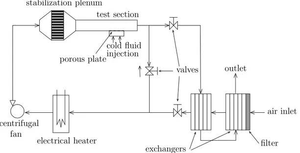
PSfrag replacements stabilization plenum porous plate test section cold fluid injection centrifugal fan electrical heater exchangers valves filter outlet air inlet
Fig. 1. Heated wind tunnel.
3 Experimental facilities
3.1 Wind tunnel
In the present study, we focus on the blowing process and its impact on a hot turbulent wall flow. Experiments are conducted in a heated subsonic wind tunnel with a rectangular test section of 0.2 m x 0.5 m (see Fig. 1). A boundary layer first develops along a 1.3 meters long impermeable wall (see Fig. 2). Then, this turbulent boundary layer flows over a porous wall of dimensions 20 cm x 30 cm. At the beginning of the impermeable plate, a small cylinder of 2 mm diameter is placed, which permits to trigger the turbulent transition of the boundary layer at a fixed location in the wind-tunnel.
The secondary air flow is injected uniformly through the porous wall thanks to a plenum located below the plate. The injected mass flow rate is measured using a pressure-reducing orifice. The porous material is composed of sintered-stainless-steel and has a porosity of about 30 %. The average diameter of the pores is about 20 µm and the average surface roughness of the plate is nearly 5 µm.
The main flow velocity can be adjusted within the range of [0, 30] m.s−1 and the
velocity residual has been measured to be always below 1 % in the mainstream (see [14] for more details). In this study, we choose a main velocity of U∞ = 10 m.s−1
(which corresponds to a Reynolds number of about 750, 000 at the beginning of the porous plate). The main flow temperature can vary from the ambient to 500 K thanks to a 120 kW electrical heating generator. Thermal control is ensured by heating needles driven by a PID regulator. The temperature gap between the hot flow and the cold one is chosen to satisfy two main constrains. First, we want to validate our anemometry measurements set-up with a moderate temperature difference. In fact, the hot wire response is very sensitive to the temperature and the measurements are largely biased if no well-adapted temperature correction is applied. Furthermore, we want to use our experimental results to validate our large Eddy Simulations. As the theoretical approach is based on the Boussinesq approximation, the numerical results are not valid for a temperature difference greater than 30 K for air. Consequently, the main flow temperature T∞ is set to have a temperature difference between the
main flow and the injected one, ∆T = T∞− Tinj, equal to 20 K. The temperature
fluctuations are measured to be less than 0.2 K in the mainstream.
The blowing ratio, or injection rate, F , represents the amount of coolant injected in comparison to the main flow rate. It is defined as:
F = ρinjUinj ρ∞U∞
(1)
where ρ is the density, U the velocity, subscript inj refers to the injected fluid and subscript ∞ to the main fluid.
PSfrag replacements
turbulent hot flow
impermeable wall
porous wall
cold fluid inlet
turbulent boundary layer
U∞, T∞
Uinj, Tinj
x y z
Fig. 2. General configuration.
3.2 Velocity and temperature measurements
Cold and hot wires anemometry is used to measure the temperature and velocity signals but also the temperature-velocity and velocity-velocity correlations. We con-sider a triple wires probe with one cold wire and two crossed hot wires. The cold wire is mounted on a Dantec 55P01 type support and is a 1 µm diameter Pt/Rh (10 %) Wollaston wire, with about 1 mm long sensitive wire. A cross support (Dantec 55P51) is used for the hot wires, which are 5 µm diameter Pt/Rh (10 %) Wollaston wires, with about 1 mm long sensitive wire. A mechanical system enables the wire supports to stand together and close. The wires are disposed as shown in Fig. 3. It permits to measure the longitudinal (u) and vertical (v) velocity components at the same place than the temperature. Note that the wires are separated by about 1 mm, which permits to neglect the influence from one wire to another. In order to minimize the effects of space integration induced by finite dimensions of both cold and hot wires, they are placed parallel to the wall, along the transverse direction (z) that is an homogeneity direction of the turbulent flow. The probes are fixed on a traversing mechanism allowing to move them in the direction normal to the wall with an accuracy of 10 µm.
The hot wire probe is driven by a 90C10 CTA Dantec module and the cold wire probe by a 90C20 CCA Dantec module. Data are acquired through an AT-MIO-16E10
Fig. 3. Three wires support disposition (Dantec 55P51 and 55P01).
National Instruments A/D card. Hot-wires probes are calibrated in velocity with a Pitot tube combined with a high sensitivity Furness FCO332 differential pressure transmitter. Its accuracy is better than 1 % of the measured value throughout its [0 − 100] Pa range with a 0.1 Pa resolution. The cold wire probe is calibrated using a miniature Pt100 probe (PTFC101A) of 0.01 K accuracy. The wall temperature is measured with a K-type thermocouple welded onto the surface. Using an IR camera, it has previously been proved not to disrupt the temperature field of the porous surface [2].
As the frequency response of the cold wire is not ideal, we have to correct the temperature signal given by the wire. Taking into account many works on cold wire response [12, 13, 17] and our wire characteristics, we have estimated the frequency response H(f ) of the probe [3]. Then, the measured temperature spectrum is directly corrected by this function H(f ). The profiles of the temperature fluctuations are divided by a factor H = 0.89, which is calculated so that:
H2 Z ∞ 0 c T2(f ) df = Z ∞ 0 H 2 (f )Tc2(f ) df (2)
where the temperature spectrum T (f ) has been measured in our configuration tob be representative of our temperature measurements.
4 Wires calibration methods
4.1 Cold wire calibration
For the calibration of the cold wire, the voltage is assumed to vary linearly with the wire temperature, which can be considered to be equal to the temperature of the flow rounding the wire (theoretically there is less than 0.04 K difference for that wire in our configuration). The linearity has been checked in our configuration (I = 0.1 mA, R = 100.3 Ω). We measure a sensitivity ∂E/∂T = 3.15 10−2V.K−1, which leads to
a temperature coefficient of α = 1.57 10−3K−1 (to be compared with the tabulated
value at 293 K: αo = 1.60 10−3K−1). With the 12 bits A/D card within [0, 10] V,
the sensitivity of the temperature measurement can be estimated to 0.02 K.
4.2 Hot wires calibration with velocity and temperature
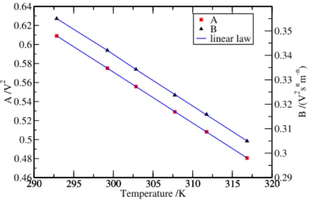
In the main flow, pressure variations within the boundary layer are negligible in comparison with the density variations due to the temperature gradient normal to the wall. Thus, the hot wire response is mainly sensitive to the local velocity and temperature of the flow. Fig. 4(a) shows an example of calibration curves obtained for various values of T∞. These measures give a calibration law in agreement with
King’s law [7]:
E2
hw = A(T ) + B(T )Un (3)
where A, B and n are King’s law coefficients. These coefficients are determined using a least squares minimizing method. As the coefficients depend on each other, an iterative technique is employed. The exponent n varies within [0.45, 0.48] and variation laws of the coefficients A and B are difficult to model. Consequently, as
2 4 6 8 Un /(mn.s-n) 0 10 20 30 40 50 60 E 2 /V 2 T = 292.8 K T = 299.2 K T = 302.8 K T = 307.7 K T = 311.7 K T = 316.8 K symbols: measurements
lines: King’s law
Fig. 4(a). Hot wires calibration (symbols : measurements, lines : King’s law).
290 295 300 305 310 315 320 Temperature /K 0.46 0.48 0.5 0.52 0.54 0.56 0.58 0.6 0.62 0.64 A /V 2 A B linear law 290 295 300 305 310 315 3200.29 0.3 0.31 0.32 0.33 0.34 0.35 B /(V 2 s n m -n )
Fig. 4(b). A and B coefficients evolution with the temperature (n = 0.46).
fil 1 fil 2 PSfrag replacements α1 α2 y θ ~ U U V x y z U⊥1 Uk1 U⊥b1 U⊥2 Uk2 U⊥b2
Fig. 5. Wires and laboratory referentials.
noticed by [5], we fix the exponent n independently of the temperature and the mean value calculated for all the temperatures is retained. We then fix n to a value of 0.46 for the first wire and 0.47 for the second one. Using these values for n, the coefficients A and B are calculated, for each value of the mean temperature, with the iterative least squares method and are observed to vary linearly with the flow temperature (see Fig. 4(b)). Note that the error between the calculated values and the linear law is lower than 0.5 %. For the wire i (i = 1 or i = 2), the evolution of Ai and Bi is written: Ai = Ai;0+ Ai;1T and Bi = Bi;0+ Bi;1T . The values of all the
coefficients are given in Table 1.
For the angle calibration of the crossed hot wires, a cosinus method [6] is employed. King’s law is written using an effective velocity defined as:
hot wire 1 hot wire 2 n1= 0.46 n2= 0.47 α1 = 49.3o α2 = 49.7o k1 = 0.17 k2 = 0.15 A1;0= 4.15 V2 A2;0 = 4.32 V2 A1;1= −8.78 10−3V2.K−1 A2;1 = −9.63 10−3V2.K−1 B1,0= 0.529 V2.s0.46.m−0.46 B2,0 = 0.629 V2.s0.47.m−0.47 B1;1= −0.97 10−3V2.s0.46.m−0.46.K−1 B2;1 = −1.20 10−3V2.s0.47.m−0.47.K−1 Table 1
Calibration coefficients for the two hot wires.
U2
e = U⊥2 + k2Uk2 (4)
where U⊥ and Uk are respectively the orthogonal and parallel velocity as far as
the wire axis is considered. If αi is the angle between the lab vertical and wire i
direction, the angle calibration with a least square minimization method leads to the coefficients values given in Table 1.
4.3 Velocity components determination
Due to the non-linearity of the equation between the velocity components expressed in the laboratory referential and in the wire referential, the inversion is not obvious and the difficulty comes from the introduction of the ki parameters. Without these
Ue,1 Ue,2 = M. U V (5)
where M is defined as:
M = cos α1 sin α1 − cos α2 sin α2 (6)
Consequently, we can express the velocity in the lab referential by inversion of the matrix M .
When parameters ki are considered, it leads to the following equations:
Ue,12 = a1U2 + b1U V + c1V2 (7) U2 e,2 = a2V2+ b2V U + c2U2 (8)
where a1,2, b1,2 and c1,2, are defined as:
a1 = (cos α1)2+ k12(sin α1)2 (9) b1 = 2(1 − k21) cos α1sin α1 (10) c1 = (sin α1)2+ k21(cos α1)2 (11) a2 = (sin α2)2+ k22(cos α2)2 (12) b2 = 2(k22− 1) cos α2sin α2 (13) c2 = (cos α2)2+ k22(sin α2)2 (14)
When considering V constant (resp. U constant) in Eq. (7) (resp. in Eq. (8)), one obtains a second order equation with two real solutions. But in both cases, only
one solution has a physical basis and, as a consequence, it leads to the following expressions of U and V : U = −b1V + q b2 1V2− 4a1(c1V2− Ue,12 ) 2a1 (15) V = −b2U + q b2 2U2− 4a2(c2U2 − Ue,22 ) 2a2 (16)
An iterative method is employed to determine U and V with an initialization of the method with the solution calculated for ki = 0. We observe that the calculation
rapidly converges after four or five iterations.
5 Preliminary measurements
5.1 Influence of the temperature on the hot wire
As noticed before, the temperature has an impact on the hot wires responses. This influence can be estimated by the sensitivity coefficients of the hot wires. In fact, we can estimate the change in the velocity induced by the temperature gap of our configuration (∆T = 20 K) by:
St∆T /Su ' 4 m.s−1 (17)
where St = ∂E/∂T and Su = ∂E/∂U are the temperature/velocity sensibility
coef-ficients of the wire. Therefore, the temperature correction of King’s law coefcoef-ficients appears very important here.
The study of the temperature influence on the hot wires in our configuration shows very little differences on the mean velocity profiles. In contrast, the velocity
fluctu-0 0.02 0.04 0.06 0.08 0.1 0.12 y /m 0 0.2 0.4 0.6 0.8 1 1.2 1.4 1.6 1.8 2 2.2 Urms /(m.s -1 ) F = 1.0 % F = 3.0 % F = 5.0 % - symbols : A(Tm), B(Tm) - no symbol : A(T), B(T)
Fig. 6(a). Velocity fluctuations with instan-taneous or mean temperature correction for A and B. 0 0.02 0.04 0.06 0.08 0.1 0.12 y /m 0 0.5 1 1.5 2 2.5 3 3.5 4 Trms /K and error x 15 F = 1.0 % F = 3.0 % F = 5.0 % - symbols : error x 15 - no symbol : Trms
Fig. 6(b). Correlation between temperature fluctuations and error in velocity fluctua-tions estimation.
ations are significantly underestimated without the correction of the coefficients A and B to take the instantaneous temperature into account. We have reported on Fig. 6(a) the velocity fluctuations profiles for three injection rates when considering the instantaneous temperature correction for King’s coefficients (A(T ) and B(T )) or not (A(Tm) and B(Tm)). In the latter case, King’s coefficients are taken at the
mean temperature Tm calculated at each wire position in the boundary layer during
a separate set of measurements. We can notice a nearly 30 % error in the estimation of the velocity fluctuations level when no instantaneous temperature correction is considered. These differences come from the possibility (or not), for the the coeffi-cients A and B, to vary with the temperature fluctuations. Indeed, Fig. 6(b) shows the correlation between the temperature fluctuations and the errors in the velocity fluctuations profiles of Fig. 6(a).
These observations point out the importance of measuring simultaneously the instan-taneous velocity and temperature in order to well estimate the velocity fluctuations levels.
5.2 Influence of the Seebeck effect on the cold wire response
Even if the cold wire gives access to a scalar (and not to a vector like the hot wires), its position must be chosen carefully. In fact, the features of the spatial evolution of the temperature (such as an isothermal direction) should help to find a good position for this wire. More precisely, one should be carreful to the Seebeck effect that appears at the wires’ junctions (PtRh-Ag and Ag-Steel prong in our case).
In our configuration, two positions of the cold wire are questioning. On the one hand, in order to minimize the Seebeck effect, the wire should be parallel to the transverse axis z. On the other hand, the vertical position, along y axis, would give access to a better location for the measurement of the temperature and velocity since hot and cold wire can be closer (about 1 mm between each wire). In our configuration, we have chosen the second position to get the better localized measures and we correct the Seebeck effect.
This correction comes from a comparison between the measurements from the three wires probe (described previously) and a two wires probe. This latter has a cold wire and a hot wire that are parallel, close and placed along transverse axis, so that the Seebeck effect can be neglected. The mean temperature profiles from these two probes are plotted on Fig. 7(a). The differences correspond to the temperature gradi-ent level and are a characteristic of the Seebeck effect. We can estimate the Seebeck coefficient by plotting the difference of voltage between the two cold wires divided by the wires length L and the temperature gradient. We take here as wire length L = 3 mm, because it corresponds to the distance between the junctions Ag-Steel prongs, which have a higher thermoelectrical effect than the PtRh-Ag junctions. We observe on Fig. 7(b) the thermoelectrical effect on the vertical cold wire. Note that an unique value for all injection rates can hardly be obtained, since the temperature gradient between the two junctions is not constant in time. In fact, we have
consid-0 0.02 0.04 0.06 0.08 0.1 0.12 y /m 0 0.2 0.4 0.6 0.8 1 (Tm - T inj ) / ∆T F = 0.0 % F = 0.5 % F = 1.0 % F = 2.0 % F = 3.0 % F = 5.0 % - straight lines: 3 wires probe - dashed lines: 2 wires probe
Fig. 7(a). Mean temperature profiles with the 2 and 3-wire probes.
0 0.01 0.02 0.03 0.04 y /m -80 -60 -40 -20 0 20 40 [ Em,2fils - E m,3fils ] / [ L . ( ∂Tm /∂ y) ] /( µV.K -1 ) F = 1 % F = 2 % F = 3 % F = 5 %
Fig. 7(b). Thermoelectrical effect on the vertical cold wire.
ered a mean gradient and no variation in time. The phase change of the temperature fluctuations between the two junctions cannot be neglected. Indeed, the tempera-ture difference between the two junctions due to the mean temperatempera-ture gradient can be evaluated to ∆T ' ∂Tm
∂y L ' 1.5 K, whereas the temperature difference due
to the phase change can be estimated to ∆T ' Trms ' 2 K (for phase opposition).
Consequently, the Seebeck effect in our configuration may come from both mean gradient and phase change of the temperature signal. Note here that the Seebeck effect from phase changes also exists when the cold wire is placed along isothermal lines.
When the fluctuations profiles of the temperature and the velocity from the two probes are compared, we observe little discrepancies (less than 3 % for F < 5 %, and less than 6 % for F = 5 %). Consequently, in our configuration the main con-sequence of the Seebeck effect is the modification of the mean profiles. Since the mean temperature profiles are misestimated, the mean velocity profiles are also mis-estimated due to the calibration laws for A(T ) and B(T ). Therefore, we consider in the following the mean temperature signal of the ”three wires probe” corrected by the mean temperature signal from the ”two wires probe”. Doing so, the mean temperature profiles from the two probes fit exactly, and the mean velocity profiles
correspond very well (less than 2 % error).
6 Results and discussion of the blowing process
In this section, we present the experimental results of non-isothermal blowing through the porous plate. The injection rate varies from 0% (no injection) to 5%. We first present the impact of the blowing at the wall, then we investigate its influence on the boundary layer.
6.1 Effect of the blowing at the wall
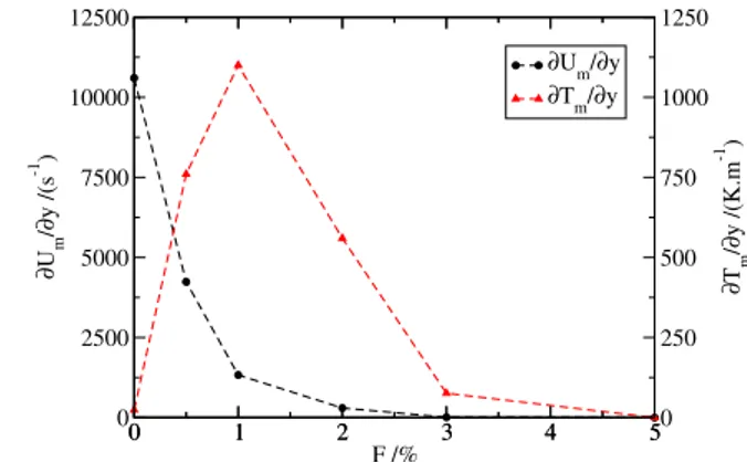
Fig. 8 presents the evolution of the wall temperature for several injection rates. These results are obtained both using thermocouples and extrapolating the results of the cold wire. We can first observe that we have a very good agreement between the two methods. When the blowing is applied, the mean wall temperature is significantly reduced even for weak injection rates. The temperature fluctuations are also very important at the wall since they can damage it, even if the mean wall temperature is low. Fig. 16 shows that near the wall the temperature fluctuations increase with the blowing rate but remain low (≤ 2 K) in all cases.
In Fig. 9, the wall gradients of the velocity and the temperature are displayed. Concerning the velocity, we note a continuous decrease of the gradient, and as a consequence of the wall shear stress (τw = µ∂U∂y|y=0) and the friction coefficient
(Cf = τw
1/2ρU2), when the blowing rate increases. This decrease is first very important,
then the gradient tends to zero, which corresponds to the blow off of the boundary layer. The behaviour of the temperature gradient is more delicate. First, the gradient increases for weak blowing rates (F lower than 1%). Then it decreases for higher injection rates. For a weak blowing ratio, the wall temperature is highly decreased,
whereas the temperature of the near-wall flow is not much modified. Consequently, it induces a high temperature difference between the wall and the flow that is close to the wall, and thus a high temperature gradient. For higher injection rates, the blowing decreases the temperature of the flow above the wall as well as the wall temperature (development of a cold fluid film), leading to a temperature of the same order of magnitude than the injected fluid. The temperature gradient is thus reduced. 0 1 2 3 4 5 F /% 290 295 300 305 310 315 Tw /K cold wire thermocouple
Fig. 8. Wall temperature measured with a ther-mocouple and by extrapolation from cold wire.
0 1 2 3 4 5 F /% 0 2500 5000 7500 10000 12500 ∂Um /∂ y /(s -1 ) 0 1 2 3 4 50 250 500 750 1000 1250 ∂Tm /∂ y /(K.m -1 ) ∂Um/∂y ∂Tm/∂y
Fig. 9. Velocity and temperature gradients at the wall.
6.2 Influence of the blowing on the boundary layer
When blowing is applied, the boundary layers are affected. The blowing increases both the dynamic and thermal boundary layers as it can be seen in Fig. 10. We can remark that the thickness of the two boundary layers are equal and that they are similarly affected by the blowing. We also plotted the position of the maximum of the velocity fluctuations as a function of the blowing rate. We observe that it increases with the blowing and its evolution is almost linear. It follows the increase of the boundary layer thickness.
The mean longitudinal and vertical velocity profiles are presented in Fig. 11 and 13. The two profiles are disturbed by the injection. The longitudinal velocity is
de-0 1 2 3 4 5 F /% 0 0.01 0.02 0.03 0.04 0.05 0.06 0.07 δ /m δU δT ymax Urms
Fig. 10. Boundary layer thickness evolution with F .
creased, whereas the vertical one is increased, for a constant vertical position in the boundary layer. We can also remark that the shape of the longitudinal velocity is modified for high injection rates, illustrating another behaviour of the velocity field. The trend is logarihtmic without injection and becomes almost linear for high blowing rates.
The longitudinal and vertical velocity fluctuations are strongly modified by the blow-ing, as it can be observed in Fig. 12 and 14. The levels of these fluctuations increase when the injection rate increases, except at the wall, where they slightly decrease. Furthermore, the peak of the fluctuations is shifted away from the wall. We can also remark that the width of the peak is spreaded, showing that the region where the turbulent mixing takes place widens.
Concerning the temperature, we can first note that the mean temperature (Fig. 15) is affected. The temperature is reduced and we note, as for the velocity, that the shape is modified for high injection rates (from a logarithmic to a linear trend). The temperature fluctuations (Fig. 16) are dramatically affected by the blowing. Their increase is very important. Their peak is also shifted but, at the opposite of the velocity fluctuations, their level near the wall slightly increases. The shape of these profiles changes, especially for the highest blowing rates.
0 0.02 0.04 0.06 0.08 0.1 0.12 y /m 0 0.2 0.4 0.6 0.8 1 Um / U ∞ F = 0.0 % F = 0.5 % F = 1.0 % F = 2.0 % F = 3.0 % F = 5.0 %
Fig. 11. Mean longitudinal velocity.
0 0.02 0.04 0.06 0.08 0.1 0.12 y /m 0 0.2 0.4 0.6 0.8 1 1.2 1.4 1.6 1.8 Urms /(m.s -1 ) F = 0.0 % F = 0.5 % F = 1.0 % F = 2.0 % F = 3.0 % F = 5.0 %
Fig. 12. Longitudinal velocity fluctuations.
0 0.02 0.04 0.06 0.08 0.1 0.12 y /m 0 0.2 0.4 0.6 0.8 1 1.2 1.4 1.6 1.8 Vm /(m.s -1 ) F = 0.0 % F = 0.5 % F = 1.0 % F = 2.0 % F = 3.0 % F = 5.0 %
Fig. 13. Mean vertical velocity.
0 0.02 0.04 0.06 0.08 0.1 0.12 y /m 0 0.2 0.4 0.6 0.8 1 1.2 Vrms /(m.s -1 ) F = 0.0 % F = 0.5 % F = 1.0 % F = 2.0 % F = 3.0 % F = 5.0 %
Fig. 14. Vertical velocity fluctuations.
0 0.02 0.04 0.06 0.08 0.1 0.12 y /m 0 0.2 0.4 0.6 0.8 1 (Tm - T eff ) / ∆T F = 0.0 % F = 0.5 % F = 1.0 % F = 2.0 % F = 3.0 % F = 5.0 %
Fig. 15. Mean temperature.
0 0.02 0.04 0.06 0.08 0.1 0.12 y /m 0 0.5 1 1.5 2 2.5 3 3.5 4 4.5 5 Trms /K F = 0.0 % F = 0.5 % F = 1.0 % F = 2.0 % F = 3.0 % F = 5.0 %
On both the mean longitudinal velocity and temperature profiles, we can see the increase in the boundary layers thickness previously noticed. We also observe a change in concavity around y = 0.005 m at F = 3% and around y = 0.02 m at F = 5%, which is characteristic of the blow-off of a boundary layer. Indeed, it shows that a low-speed and low-temperature fluid layer forms above the porous plate. The blow-off phenomenon also influences the mean vertical velocity profiles, the shape of which changes for F ≥ 3%.
The skewness and flatness factors for the longitudinal and vertical velocity as well as the temperature are given in Fig 17 to 22. Without blowing the flow statistics are nearly Gaussian, with S ≈ 0 and F ≈ 3. The skewness and flatness factors deviate from these values when blowing is applied. This reveals decentered and spreaded flow statistics. The evolution of the temperature skewness and flatness factors is gradual. For the two highest injection rates, the longitudinal velocity skewness and flatness profiles display peaks at about y = 0.005 m (F = 3% ) and y = 0.02 m (F = 5%), which corresponds to the size of the low-speed fluid film. This change in the statistics of the longitudinal velocity can therefore be seen as another sign of the blow-off of the boundary layer. SV and FV profiles also show an important
0 0.02 0.04 0.06 0.08 0.1 0.12 y /m -3 -2 -1 0 1 2 3 4 5 SU F = 0.0 % F = 0.5 % F = 1.0 % F = 2.0 % F = 3.0 % F = 5.0 %
Fig. 17. Skewness factor SU.
0 0.02 0.04 0.06 0.08 0.1 0.12 y /m 1 3 10 40 FU F = 0.0 % F = 0.5 % F = 1.0 % F = 2.0 % F = 3.0 % F = 5.0 %
Fig. 18. Flatness factor FU.
0 0.02 0.04 0.06 0.08 0.1 0.12 y /m -2 0 2 4 SV F = 0.0 % F = 0.5 % F = 1.0 % F = 2.0 % F = 3.0 % F = 5.0 %
Fig. 19. Skewness factor SV.
0 0.02 0.04 0.06 0.08 0.1 0.12 y /m 0 10 20 30 40 50 FV F = 0.0 % F = 0.5 % F = 1.0 % F = 2.0 % F = 3.0 % F = 5.0 %
Fig. 20. Flatness factor FV.
0 0.02 0.04 0.06 0.08 0.1 0.12 y /m -14 -12 -10 -8 -6 -4 -2 0 2 4 ST F = 0.0 % F = 0.5 % F = 1.0 % F = 2.0 % F = 3.0 % F = 5.0 %
Fig. 21. Skewness factor ST.
0 0.02 0.04 0.06 0.08 0.1 0.12 y /m 1 3 10 100 FT F = 0.0 % F = 0.5 % F = 1.0 % F = 2.0 % F = 3.0 % F = 5.0 %
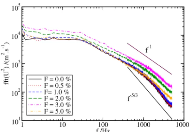
Fig. 23 to 27 present the velocity and temperature spectra for several injection rates and different positions in the boundary layer. Without injection, we find that the velocity spectrum slope is close to the classical −5/3 Kolmogorov value. This slope is modified by the blowing. The effect is not very clear for weak injection rates but is evident for higher blowing rates. In particular, for a blowing rate of 5%, the slope is decreased and reaches a value close to −1 (see Fig. 23). It is also interesting to see that the level of the spectrum evolves with the position when the flow is submitted to blowing, whereas it does not in the case without blowing (see Fig. 24 and 25).
Concerning the temperature spectrum, we observe a slope in the inertial range equal to −5/3. At the opposite of the velocity spectrum, we do not have a clear influence of the blowing on the slope (see Fig. 26 and 27). A slight influence on the level can be noted, but it remains limited. Nevertheless, we have to remind that the temperature difference is weak (≤ 20 K) and we can imagine that a stronger blowing effect could be observed with wider temperature ranges.
In Fig. 28 to 30 we can see the velocity-temperature and velocity-velocity correla-tions. As for the velocity and temperature fluctuations, the peaks of the correlations are increased and shifted away from the wall with increasing blowing rate. On the velocity-velocity correlation profile we observe a change in sign for F ≥ 3%. Again, this shows that the near-wall turbulence is strongly modified when the boundary layer is blown off.
1 10 100 1000 10000 f /Hz 101 102 103 104 105 fft(U 2 ) /(m 2 .s -1 ) F = 0.0 % F = 0.5 % F= 1.0 % F = 2.0 % F = 3.0 % F = 5.0 % f-5/3 f-1
Fig. 23. Velocity spectrum at y = 31 mm.
1 10 100 1000 10000 f /Hz 10-1 100 101 102 103 104 105 fft(U 2 ) /(m 2 .s -1 ) y = 0.2 mm y = 1.1 mm y = 3 mm y = 7 mm y = 15 mm y = 31 mm y = 51 mm y = 71 mm y = 103 mm f-5/3
Fig. 24. Velocity spectrum for F = 0.0 %.
1 10 100 1000 10000 f /Hz 10-1 100 101 102 103 104 105 fft(U 2 ) /(m 2 .s -1 ) f-5/3 f-1
Fig. 25. Velocity spectrum for F = 5.0 %.
1 10 100 1000 10000 f /Hz 100 101 102 103 104 105 106 fft(T 2 ) /(K 2 .s) y = 0.2 mm y = 1.1 mm y = 3 mm y = 7 mm y = 15 mm y = 31 mm y = 51 mm y = 71 mm y = 103 mm f-5/3
Fig. 26. Temperature spectrum for F = 0.0 %.
1 10 100 1000 10000 f /Hz 100 101 102 103 104 105 106 fft(T 2 ) /(K 2 .s) f-5/3
0 0.02 0.04 0.06 0.08 0.1 0.12 y /m 0 1 2 3 4 5 U’T’ /(m.K.s -1 ) F = 0.0 % F = 0.5 % F = 1.0 % F = 2.0 % F = 3.0 % F = 5.0 % Fig. 28. U0T0 correlation. 0 0.02 0.04 0.06 0.08 0.1 0.12 y /m -0.5 0 0.5 1 1.5 2 2.5 -V’T’ /(m.K.s -1 ) F = 0.0 % F = 0.5 % F = 1.0 % F = 2.0 % F = 3.0 % F = 5.0 % Fig. 29. −V0T0 correlation. 0 0.02 0.04 0.06 0.08 0.1 0.12 y /m -0.2 -0.1 0 0.1 0.2 0.3 0.4 U’V’ /(m 2 .s -2 ) F = 0.0 % F = 0.5 % F = 1.0 % F = 2.0 % F = 3.0 % F = 5.0 % Fig. 30. U0V0 correlation.
7 Conclusions
The experimental study of a boundary layer submitted to non-isothermal blowing has been presented. Different probes were used. A probe with two crossed hot wires and a cold hot wire allowed simulataneous measurements of the instantaneous ve-locity and temperature. The study showed that the calibration procedure is delicate due to the temperature difference. By the following, we determined the influence of the blowing on the dynamic and thermal boundary layers. We observed that the blowing modifies the velocity and temperature profiles but also the turbulent fluctu-ations. In particular, we measured the double correlations of turbulence submitted to non-isothermal blowing. In all the cases, the turbulent quantities are increased but their peaks are shifted away from the wall. Furthermore, we noticed that the blowing modifies the velocity and temperature spectra. We also observed that the blow-off of the boundary layer induces a change in the near-wall turbulence. Finally, these results will be useful for the numerical study of the blowing and will permit new developments of Thermal Large Eddy Simulation (see Part II).
References
[1] J. Bellettre, F. Bataille, and A. Lallemand. A new approach for the study of turbulent boundary layers with blowing. International Journal of Heat and Mass Transfer, 42(15):2905–2920, 1999.
[2] J. Bellettre, F. Bataille, J.-C. Rodet, and A. Lallemand. Thermal behaviour of porous plates subjected to air blowing. AIAA Journal of Thermophysics and Heat Transfert, 14(4):523–532, 2000.
[3] G. Brillant. Simulations des grandes ´echelles thermiques et exp´eriences dans le cadre d’efffusion anisotherme. Th`ese de Doctorat, INSA de Lyon, 2004.
boundary layer with blowing. Theoretical and Computational Fluid Dynamics (to appear), 2004.
[5] H. H. Bruun. Hot-wire anemometry. Principles and signal analysis. Oxford science publications, 1995.
[6] H. H. Bruun, .N Nabhani, H. H. Al-Kaylem, A. A. Fardad, M. A. Khan, and E. Hogarth. Calibration and analysis of x hot-wire probe signals. Meas. Sci. Technol., 1:782–785, 1990.
[7] L. V. King. On the convection of heat from small cylinders in a stream of fluid: Determination of the convection constants of small platinium wires with applications to hor-wire anemometry. Phil. Trans. Roy. Soc., A214:373–432, 1914.
[8] M. Marchand, J-G. Galier, P. Reulet, P. Chomdej, and P. Millan. Infrared measurements of heat transfer in jet impingement on concave wall applied to anti-icing. In 6th International Conference on Quantitative Infrared Thermog-raphy, Dubrovnik, septembre 2002.
[9] L. Mathelin, F. Bataille, and A. Lallemand. Blowing models for cooling surfaces. International Journal of Thermal Sciences, 40(11):969–980, 2001.
[10] L. Mathelin, F. Bataille, and A. Lallemand. Near wake of a circular cylinder submitted to blowing - i boundary layers evolution. International Journal of Heat and Mass Transfer, 44:3701–3708, 2001.
[11] L. Mathelin, F. Bataille, and A. Lallemand. Near wake of a circular cylinder submitted to blowing - ii impact on the dynamics. International Journal of Heat and Mass Transfer, 44:3701–3708, 2001.
[12] P. Paranthon and J. C. Lecordier. Mesures de temprature dans les coulements turbulents. Revue G´en´erale de Thermique, 35:283–308, 1996.
[13] A. Petit, P. Paranthon, and J. C. Lecordier. Influence of wollaston wire and prongs on the response of cold wires at low frequencies. Letters in Heat and Mass Transfer, 8:281–291, 1981.
[14] J.-C. Rodet, G. A. Campolina Franca, P. Pagnier, R. Morel, and A. Lallemand. ´etude en soufflerie thermique du refroidissement de parois poreuses par effusion de gaz. Revue G´en´erale de Thermique, 37(2):123–136, 1998.
[15] N. Shima. Prediction of turbulent boundary layers with a second-moment clo-sure: part i - effects of periodic pressure gradient, wall transpiration and free-stream turbulence. Journal of Fluid Engineering (ASME), 115(1):56–63, 1993. [16] A. P. Silva-Freire, D. O. A. Cruz, and C. C. Pellegrini. Velocity and temperature distributions in compressible turbulent boundary layers with heat and mass transfer. International Journal of Heat and Mass Transfer, 38(13):2507–2515, 1995.
[17] T. Tsuji, Y. Nagano, and M. Tagawa. Frequency response and instantaneous temperature profile of cold-wire sensors for fluid temperature fluctuation mea-surements. Experiments in Fluids, 13:171–178, 1992.
[18] D. G. Whitten, R. J. Moffat, and W. M. Kays. Heat transfer to a turbulent boundary layer with non-uniform blowing and surface temperature. In 4th Inter. heat transfer conf, 1970.