HAL Id: hal-01392913
https://hal.archives-ouvertes.fr/hal-01392913
Submitted on 5 Nov 2016
HAL is a multi-disciplinary open access
archive for the deposit and dissemination of
sci-entific research documents, whether they are
pub-lished or not. The documents may come from
teaching and research institutions in France or
abroad, or from public or private research centers.
L’archive ouverte pluridisciplinaire HAL, est
destinée au dépôt et à la diffusion de documents
scientifiques de niveau recherche, publiés ou non,
émanant des établissements d’enseignement et de
recherche français ou étrangers, des laboratoires
publics ou privés.
Radiation efficiency optimization of electrically small
antennas: Application to 3D folded dipole
Francois Sarrazin, Sylvain Pflaum, Christophe Delaveaud
To cite this version:
Francois Sarrazin, Sylvain Pflaum, Christophe Delaveaud. Radiation efficiency optimization of
electri-cally small antennas: Application to 3D folded dipole. International Workshop on Antenna Technology
(IWAT 2016), Feb 2016, Cocoa Beach, FL, United States. pp.29-32, �10.1109/IWAT.2016.7434792�.
�hal-01392913�
CEA-Léti, Minatec Campus Grenoble, France francois.sarrazin@cea.fr
Abstract—This paper deals with the radiation efficiency
optimization of Electrically Small Antennas (ESAs). Based on the well-known tradeoff between antenna maximum dimensions, Q-factor and radiation efficiency, several authors focused on minimizing the Q-factor for a given antenna size in order to increase its bandwidth. For some applications (Wireless Sensor Network), only a narrow bandwidth is needed and the radiation efficiency is a crucial parameter to shrink the required power. Thus, this paper presents the radiation efficiency optimization of 3D folded dipole antennas for a given size. First, we compare different folding topologies and then we study the effect of the wire diameter and the material on the ESAs performances.
Keywords—3D folding, dipole antenna, electrically small antenna, quality factor, radiation efficiency
I. INTRODUCTION
Electrically Small Antennas (ESAs) are of interest for a long time since it is a key element for radio communication systems miniaturization. Their radiation properties have been first studied in the middle of the 20th century by Wheeler [1]-[2]. In
[1], the definition of an Electrically Small Antenna (ESA) is given as < 0.5 where is the wavenumber and is the radius of the smallest sphere that encloses the antenna, also known as the Chu sphere. Based on the spherical mode wavefunction expansions outside the Chu sphere, Chu [3] showed that the quality factor of an antenna is lower bounded by its physical size such as
+ = 3 ) ( 1 1 ka ka Qlb ηrad . (1)
where is the radiation efficiency. This expression can be simplified as in (2) for ESAs ( < 0.5) which is confirmed later by McLean in [4]. 3 ) (ka Qlb rad = η . (2)
Also, it is shown in [5] that the quality factor of a narrowband antenna is inversely proportional to its bandwidth ( = 1/ ). Thus, there is a tradeoff between the radiation efficiency, the antenna maximum dimension and its bandwidth. Wheeler
original work encouraged several authors to enhance the knowledge on physical limits of ESAs [5]-[7]. Recently, Gustafsson [8] suggested, based on scattering theory, lower bounds of the Q-factor on antennas of arbitrary shape. A lot of studies focused on minimizing of ESAs for a given size in order to increase the bandwidth [9]. However, for some specific applications like Wireless Sensor Networks, only a few hundreds of kHz might be enough to communicate some data. This leads to the concept of Ultra NarrowBand (UNB) Antenna where the efficiency becomes the most critical parameter, especially since the available power of the communicating node is usually very low.
In section II, we compare the radiation performances of three electrically small dipole antennas that use different folding topologies (helical, spiral and spherical) as a function of their physical sizes. S-parameters measurements of the helix antenna using a differential technique is also presented. Then, section III focus on the spherical topology and we study the effect of the wire diameter and the material conductivity on the antenna radiation efficiency.
II. 3D-FOLDED DIPOLE ANTENNAS STUDY
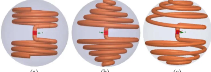
Folding is one of the most commonly used antenna miniaturization technique because of its simplicity. The main idea is to extend the current paths in a limited volume in order to reduce the resonant frequency. In the literature, several papers deal with this subject and present different structures. They can be classified into two categories: planar (2D) such as meanders, zig-zag [10], and volumetric (3D) as the helix for example [11]. In this paper, we focus only on 3D-folding by comparing the radiation properties of a helical, a spiral and a spherical dipole antennas. These antennas are presented in Fig. 1 enclosed in a
(a) (b) (c)
Fig. 1. Design of the 3D-folded dipole antennas: (a) helical, (b) spiral and (c) spherical. is equal to 0.145 for all.
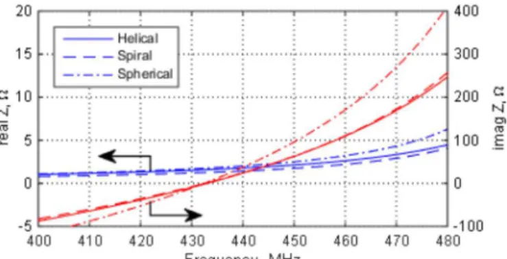
sphere of radius = 16 mm so that = 0.145.. They are optimized to operate at the same frequency of 433 MHz. The copper wires’ diameter is equal to 2 mm. The antennas are first simulated with ANSYS [12] using a 50 Ω lumped port located at the sphere’s origin. Their input impedance as a function of the frequency is presented in Fig. 2. We can see that the imaginary parts are all equal to zero at 433 MHz (serial resonances) and the real parts are very low (about 1.5 Ω) which is typical for ESAs. The impedance matching to 50 Ω is not considered in this study. The helical antenna has been realized as depicted in Fig. 3. Since this symmetrical antenna is electrically small, the classical impedance measurement setup using one coaxial cable is not suitable. Indeed, this unbalanced feeding system generates current leaking along the shield of the cable. Thus, we use a balanced measurement technique [13] based on two distinct coaxial cables. Each core is connected to an antenna arm and the two shields are soldered together as shown in Fig. 3. On the other side, the two coaxial cables are terminated by a SMA connector to be connected to the VNA. First, the VNA is calibrated in a classical way. Then, the two soldered coaxial cables are de-embedded by post-processing using the S-parameters measured when these cables are terminated by a short circuit and a 50 Ω
load. Finally, the S-parameters of the whole structure including the antenna are measured and the differential input impedance
can be computed as 21 12 22 11 22 11 21 12 0 ) 1 )( 1 ( ) 1 )( 1 ( 2 S S S S S S S S Z Zdiff − − − − − − = (3)
where is the characteristic impedance (50 Ω). Since the antenna is symmetric, we obtain = and = . The simulated and measured helix antenna input impedance is presented in Fig. 4 as a function of the frequency. We can see that they are in very good agreement.
We now analyze the simulated radiation properties of the folded dipole antennas as a function of their dimensions. Four values of have been arbitrary chosen: 0.145, 0.2, 0.25 and 0.32. For each , the three antennas are optimized to be enclosed in the Chu sphere and operate at 433 MHz ( = 0). The wires’ diameter is kept the same (2 mm). The simulated radiation efficiency and Q-factor are presented as a function of in Fig. 5 and Fig. 6, respectively, for the three different folded dipoles. First of all, the behavior of these parameters as a function of respects the theory, i.e. when shrinks, the radiation efficiency decreases while the Q-factor increases. In Fig. 5, we can see that the radiation efficiencies are the same for the highest considered ( = 90%). However, a better efficiency is obtained with the spherical folding when the antenna size becomes smaller. For = 0.145, the efficiency of the spherical antenna is 13 % higher than for the spiral antenna and 17 % higher than the helix antenna. Regarding (Fig. 6), results are very similar for
Fig. 4. Simulated and measured helix antenna input impedance.
Fig. 6. Simulated Q-factor as a function of for the three different kind of dipole antennas.
Fig. 2. Simulated input impedance of the helical, spiral and spherical antennas as a function of the frequency.
Fig. 3. Picture of the realized helix antenna connected to two coaxial cables to be measured using a differential method.
Fig. 5. Simulated radiation efficiency as a function of for the three different kind of dipole antennas.
“large” while there is a clear difference when the antenna becomes smaller. It is interesting to notice that the spherical antenna has both the highest efficiency and the smallest Q-factor.
We now focus on the ratio between the radiation efficiency and the quality factor, expressed in (2) as proportional to . Results are presented in Fig. 7. We notice that this ratio is indeed proportional to for electrically small dimensions ( < 0.01 and so < 0.2) but the slope is not the same regarding the antenna topology. A proportionality coefficient should thus be introduced into (2) such as
3 ) (ka Q rad α η = (4)
where can be seen as a figure of merit describing ESA performances as a function of its electrical volume . These results agree with recent works saying that the more the antenna fill the Chu sphere, the more this antenna is efficient. It also confirms that the ESAs radiation properties depend on the effective antenna volume [8] and not only the equivalent sphere. III. OPTIMIZATION OF THE SPHERICAL ANTENNA RADIATION
EFFICIENCY
In this section, we focus on radiation properties of the spherical antenna only by trying to improve its radiation efficiency without strongly modifying its structure. If we consider a sinusoidal current distribution along a half-wavelength dipole antenna, its loss resistance can be simplified as σ ωµ π δ π σ2 4 2 2 1 0 r l r l Rloss = = (5)
where is the dipole length, is the conductivity of the metal, is the wire radius and is the skin depth defined as =
2⁄ with the permeability of free-space and the angular frequency. Thus, increasing or should in theory reduce and so increase the radiation efficiency. These parameters have usually few influence on the efficiency of half-wavelength dipole but their effect on the specific case of ESAs is studied in the next two parts.
A. Wire diameter study
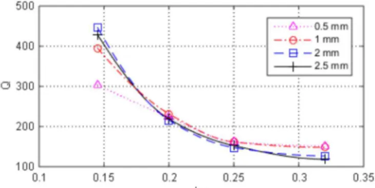
In this part, we study the effect of the wire diameter on the spherical antenna performances. Thus, we arbitrary choose two smaller diameters (0.5 mm and 1 mm) and a larger one (2.5 mm). The antennas are then optimized to operate at 433 MHz ( = 0) for each diameter. The radiation efficiency simulated for the four diameters is presented as a function of in Fig. 8 while its Q-factor is shown in Fig. 9. As previously, both results agree with the physics. We notice that the radiation efficiency is highly related to the wire diameter. Indeed, the larger the diameter, the higher the efficiency. This is true for all sizes that have been simulated but the smallest one. In this particular case of = 0.145 there is no improvement when the diameter increases from 2 mm to 2.5 mm. Indeed, since the wire diameter is increased while keeping the same overall dimension, the pitch becomes very small and disturb the antenna radiation properties. Regarding the Q-factor, for large , it is higher for the smaller diameter. This is consistent with half-wavelength dipole where the thicker the wire, the more broadband the dipole. However, when is reduced, small diameter leads to low Q and thus increased bandwidth which confirms that there is a tradeoff between efficiency and bandwidth.
Finally, the ratio / is presented as a function of for every diameters in Fig. 10. As expected from the previous results, this ratio is proportional to for very small (minor than 0.2). For higher , the thicker the wire, the better the radiation properties. Looking at the proportionality for small , we observe that the coefficient depends on the wire’s diameter. This analyze has also been done with the spiral and spherical dipole antennas and lead to the same conclusions. Results are not presented here for brevity.
Fig. 7. Simulated radiation efficiency to Q-factor ratio as a function of for the three different kind of dipole antennas.
Fig. 9. Simulated Q-factor of the spherical antenna as a function of for four different diameters.
Fig. 8. Simulated radiation efficiency of the spherical antenna as a function of for four different diameters.
B. Material study
We now focus on the effect of the material conductivity on the miniature antenna performances. The spherical antenna is simulated using four materials: brass ( = 15. 10 / ), aluminum ( = 38. 10 / ), copper ( = 58. 10 / ) and silver ( = 61. 10 / ). The simulated radiation efficiency is presented as a function of in Fig. 11 while the Q-factor is shown in Fig. 12. Whatever , the metal conductivity has an influence on the efficiency of the antenna. Indeed, the higher the conductivity, the higher the radiation efficiency. The difference is especially high since we are dealing with ESAs. Regarding it is higher for high conductivity material. Finally, we present the radiation efficiency by the Q-factor ratio as a function of in Fig. 13. It is very interesting to notice that the material conductivity has no influence on this ratio. It means that the coefficient introduced in (4) does not depend on the metal used and that the differences observed in Fig. 11 and Fig. 12 compensate each other perfectly.
IV. CONCLUSION
Electrically small 3D-folded dipole antennas have been studied in terms of their radiation efficiency and Q-factor. We showed that a topology that fills the best the Chu sphere gives better performances. Then we showed that, for a same effective volume, it is possible to modify the antenna radiation properties by adjusting the wire diameter or the material conductivity.
ACKNOWLEDGMENT
This work is financially supported by the French Research Agency under the project SENSAS (ANR-13-INFR-0014).
REFERENCES
[1] H. A. Wheeler, “Fundamental limitations of small antennas,” Proc. IRE, vol. 35, pp. 1479-1484, 1947.
[2] H. A. Wheeler, “The radiansphere around a small antenna,” Proc. IRE, vol. 47, pp. 1325-1331, 1959.
[3] L. J. Chu, “Physical limitation on omnidirectional antennas,” Journal of Applied Physics, vol. 19, pp. 1163-1175, 1948.
[4] J. S. McLean, “A re-examination of the fundamental limits on the radiation of electrically small antennas,” IEEE Trans. Antennas Propag., vol. 44, no. 5, pp. 672–676, May 1996.
[5] S. R. Best, “A discussion on the quality factor of impedance matched electrically small antennas,” IEEE Trans. on Ant. and Prop., vol. 53, no. 1, pp. 502-508, 2005.
[6] R. F. Harrigton, “Effect of antenna size on gain, bandwidth, and efficiency,” Journal Res. Nat. Bureau Standards, vol. 64D, pp. 1-2, 1960. [7] A. D. Yaghjian and S. R. Best, “Impedance, bandwidth, and Q of antennas,” Trans. on Ant. and Prop., vol. 53, no. 4, pp. 1298-1324, 2005. [8] M. Gustafsson, C. Sohl and G. Kristensson, “Physical limitations on antennas of arbitray shape,” Proceedings of the royal society of London A, vol. 463, no. 2086, pp. 2589-2607, 2007.
[9] N. Behdad and K. Sarabandi, “Bandwidth enhancement and further size reduction of a class of miniaturized slot antennas," IEEE Trans. on Ant. and Prop., vol. 52, no. 8, pp. 1928-1935, Aug. 2004.
[10] H. Nakano, H. Tagami, A. Yoshizawa and J. Yamauchi, "Shortening ratios of modified dipole antennas," IEEE Trans. on Ant. and Prop., vol. 32, no. 4, pp. 385-386, Apr. 1984.
[11] S. R. Best, "The radiation properties of electrically small folded spherical helix antennas," IEEE Trans. on Ant and Prop., vol. 52, no. 4, pp. 953-960, Apr. 2004.
[12] ANSYS® Electromagnetics Suite, Release 16.0.
[13] Meys, R.; Janssens, F., “Measuring the impedance of balanced antennas by an S-parameter method," IEEE Antennas and Propagation Magazine, vol. 40, no. 6, pp. 62-65, Dec. 1998
Fig. 10. Radiation efficiency to Q-factor ratio of the spherical antenna as a function of for the four different diameters.
Fig. 12. Simulated Q-factor of the spherical antenna as a function of for four different materials.
Fig. 11. Simulated radiation efficiency of the spherical antenna as a function
of for four different materials. Fig. 13. Radiation efficiency to Q-factor ratio of the spherical antenna as a function of for the four different materials.