HAL Id: hal-00719855
https://hal.archives-ouvertes.fr/hal-00719855
Submitted on 21 Jul 2012
HAL is a multi-disciplinary open access
archive for the deposit and dissemination of
sci-entific research documents, whether they are
pub-lished or not. The documents may come from
teaching and research institutions in France or
abroad, or from public or private research centers.
L’archive ouverte pluridisciplinaire HAL, est
destinée au dépôt et à la diffusion de documents
scientifiques de niveau recherche, publiés ou non,
émanant des établissements d’enseignement et de
recherche français ou étrangers, des laboratoires
publics ou privés.
multibody robots
Sébastien Rubrecht, Vincent Padois, Philippe Bidaud, Michel de Broissia,
Max da Silva Simoes
To cite this version:
Sébastien Rubrecht, Vincent Padois, Philippe Bidaud, Michel de Broissia, Max da Silva Simoes.
Motion safety and constraints compatibility for multibody robots. Autonomous Robots, Springer
Verlag, 2012, 32 (3), pp.333-349. �10.1007/s10514-011-9264-x�. �hal-00719855�
(will be inserted by the editor)
Motion safety and constraints compatibility for multibody
robots
S´ebastien Rubrecht · Vincent Padois · Philippe Bidaud · Michel de
Broissia · Max Da Silva Simoes
Received: date / Accepted: date
Abstract In this paper we propose a methodology to ensure safe behaviors of multibody robots in reactive control frameworks. The permanent satisfaction of con-straints being insufficient to ensure safety, this approach focuses on the constraints expression: the compatibility between these constraints is studied, and safe alterna-tives are ensured when compatibility cannot be estab-lished. A complete case study involving obstacles, joint position, velocity and acceleration limits illustrates the approach. A particular method is developed to take full advantage of a smooth state of the art avoidance tech-niques (Faverjon et al. 1987) while maintaining safety. Experiments involving a 6-DOF manipulator operating in a cluttered environment illustrate the reliability of the approach and validate the expected performances. Keywords Robotic constraints · Constraints compli-ant control · Motion safety · Multibody robot safety · Safe reactive control
S. Rubrecht, M. de Broissia Bouygues Travaux Publics St Quentin en Yvelines, France
E-mail: [email protected], [email protected] V. Padois, P. Bidaud
Universit´e Pierre et Marie Curie
Institut des Syst`emes Intelligents et de Robotique Paris, France
E-mail: [email protected], [email protected] M. Da Silva Simoes
Commissariat `a l’Energie Atomique et aux Energies Alterna-tives, CEA, LIST, Interactive Robotics Laboratory
Fontenay aux Roses F-92265, France E-mail: [email protected]
1 Introduction
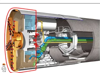
The starting point of the present work deals with the use of a robotic arm in charge of maintenance tasks in the inner part of the excavation room of a tunnel boring machine (Fig. 1). The robot is teleoperated to perform inspections and cleaning tasks in a fix and cluttered environment. The control of such a robot is reactive (teleoperation is not compatible with offline planning) and subject to real time constraints (force feedback re-quires control loop frequencies higher than 500 Hz). Al-though the features of this problem are common in the literature, safety issues remain. For example, most of the collisions avoidance methods do not take the sys-tem dynamics into account, which may cause collisions in tight environments and high speed motions. As the robot is subject to kinematic and dynamic constraints that cannot be ignored, it is important to take the phys-ical properties of the system and its environment into account to ensure motion safety.
1.1 Safety criterions for control
The notion of safety for a system is a principle applied at various levels. At the design level, safety is often inte-grated directly in the system (Ikuta et al. 2003, Zinn et
al. 2004, Haddadin et al. 2010). At the control level, the
work related to offline optimal trajectory planning is closely linked to joint constraints management (Brady 1982, Biagiotti et al. 2008); in spite of the context dif-ferences1, their recent adaptations to online frameworks
(Kr¨oger 2010) exhibit some similarities with reactive
1 most of these approaches are exclusively concerned with
joint physical limits as operational constraints are managed by path planning
Fig. 1 Tunnel Boring Machine. The red line encircles the cutter head and the excavation room, which is the manipula-tor’s working area
control techniques. In a strictly reactive context, safety has been neglected for a long time. Recently, Fraichard (2007) proposed 3 criteria to ensure safety:
1. to decide its future motion, a robotic system should consider its own dynamics;
2. to decide its future motion, a robotic system should consider the environment objects future behavior; 3. to decide its future motion, a robotic system should
reason over an infinite time-horizon.
In case of a static environment (not known a priori ), only the first criterion stands: the future behavior of the objects in the environment remains identical to the current one. The third criterion can thus be integrated in the first one if the consideration of the system’s own dynamics is done over an infinite time-horizon (referred later as the extended criterion 1 ).
1.2 Safety of common approaches for collisions avoidance with multibody robots
The number of constraints being potentially higher than the number of DOF, the usual active avoidance
tech-niques (approaches for which the avoidance requires
a motion) involved in multi-objectives frameworks (is-sued from Khatib et al. (1986) and Maciejewski et al. (1985)) cannot lead to safety. Moreover, they do not involve dynamics in the avoidance magnitude compu-tation.
Faverjon and Tournassoud (1987) proposed an avoid-ance technique included in a Quadratic Programming (QP) control law structure. This method limits the ve-locities toward obstacles by inequalities (passive avoid-ance), which is more likely to avoid the collisions what-ever the number of obstacles. QP are now widely used in manipulators or humanoids control (Decr´e et al. 2009,
Escande et al. 2010), but the avoidance methods still do not include dynamics on an infinite time-horizon. It results that, to our knowledge, no control law for multi-body robot passes the extended criterion 1.
In fact, most of the research work related to safety at the control level is led in the field of mobile robotics,
i.e. single body mobile robots avoiding collisions:
mod-els are simpler, and the operational capabilities predic-tions are easier (operational deceleration limits do not depend on the robot configuration for example). As an example, the Dynamic Window Approach (DWA) (Fox
et al. 1997) involves the acceleration limits of a mobile
robot and ensures its safety in a fix environment (ex-tended criterion 1). More recent developments in this domain are part of the framework based on the notion of Inevitable Collision State proposed by Fraichard et
al. (2004): e.g. Martinez-Gomez et al. 2009, Althoff et al. 2010, Bautin et al. 2010.
To the best of our knowledge, although this framework could be used to assess the safety of a wider scope of applications, 1/ it has never been applied to multibody robots; 2/ it is limited to collisions avoidance with re-spect to dynamics, which can be formulated as the com-patibility between the constraint of geometric collisions avoidance and acceleration limits. However, these are just two constraints among the many constraints that have to be faced in robotics: joint position, velocity, ac-celeration and torque limits (joint space), collisions with obstacles and forbidden regions (Cartesian space), con-tacts conservation constraints (Park et al. 2008), coma-nipulation and cooperation (Khatib et al. 2001), actu-ators temperature limits (Guilbert et al. 2008), etc. We can conclude that there is still a lack regarding robots safety (in particular for multibody robots) when con-sidering a large variety of constraints.
1.3 Constraints compatibility
All these constraints can be considered at the velocity kinematics level for example, where the model is tradi-tionally formulated as
˙
Xdes(t) =
∂Xdes(t)
∂q q(t) = J˙ T(q(t)) ˙q(t) (1)
where JT(q), ˙Xdes, q and ˙qare respectively the
oper-ational task Jacobian matrix (size (m, n)), the opera-tional desired velocity vector (size m), the robot config-uration (size n) and the joint space velocity vector (size n). The QP formulation of the control problem has the advantage to explicit the constraints that are supposed
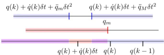
Fig. 2 Incompatibility between constraints represented in the joint space. The terms q(k) + ˙q(k)δt + ¨qm(k)δt2 and
q(k) + ˙q(k)δt + ¨qM(k)δt2are respectively the configurations
induced by a full acceleration and full deceleration (approx-imation based on finite differences). The subscripts m and M denote respectively the minimum (negative value) and the
maximum (positive value) limit of the considered variable. The control admissibility space of joint acceleration limits (up) and minimum joint position limit (middle) cannot be satisfied simultaneously: q(k + 1) ≈ q(k) + ˙q(k)δt will in-evitably violate one of the constraints
to be satisfied by the robot min
˙q (k+1)∈Rn|| ˙Xdes(k + 1) − JT(q(k)) ˙q(k + 1)|| (2)
subject to JC˙q(k + 1) − b(k) ≤ 0 (3)
where k is the current time step, ˙q(k + 1) is the velocity vector chosen for the next time step (control input vec-tor), JC is the Jacobian of constraints (size (p, n)) and
b(k) is the constraints limit vector (size p). The feasi-bility of the problem (i.e. the existence of ˙q(k + 1) such that JC˙q(k +1)−b(k) ≤ 0) is usually taken for granted;
however, if the constraints expressions have not been carefully set-up, incompatibilities may occur. The typ-ical case is the joint position limit violation because of limited accelerations illustrated by Fig. 2. If a joint gets close to one of its position limits with a high velocity, its deceleration capabilities may not be sufficient to avoid the collision with the boundary (joint position limit).
As an example, a maximum deceleration 2 rad/s2
im-posed on a joint moving at 1.0 rad/s requires 0.5 s to actually stop; then, distance travelled is 0.25 rad. This example illustrates the fact that satisfying at each time the joint position and the joint acceleration limits does not prevent from a constraint violation due to incom-patibility. Usually, virtual envelopes are set up around the physical limits to absorb such violations. These en-velopes do not guarantee safety and often artificially limit the performances of the robot. Relying on a safe approach taking dynamics into account would enable to reduce significantly those envelopes.
The contribution of this paper is to propose a method-ology to ensure safety at the control level. The control problem resolution it out of the scope of this paper: it is assumed that once the control problem is feasible, a control law algorithm such as the one proposed in Rubrecht et al. (2010a,b), solves it appropriately
(Con-straints Compliant Control law). The present work fo-cuses on the formulation of the control problem.
The proposed methodology is applied to the case of a multibody robot in a static environment (extended criterion 1). Sect. 2 exposes the description retained for the robotic system and its constraints and proposes a definition of safety at the control level. Sect. 3 is dedi-cated to the methodology description, whereas Sect. 4 details case studies dealing with static obstacles, joint positions, velocities and accelerations constraints. Fi-nally, a set of experiments illustrates the approach in Sect. 5.
2 Description for safety
In this section, an appropriate description of the robot and its constraints is introduced and a resulting def-inition of safety is proposed. In this work the control problem is formulated at the velocity kinematic level. The assumptions of this study are an exact perception of the system and the environment, an exact knowl-edge of the model and the system real capabilities and an exact execution when the desired joint input satis-fies the constraints: u(k) = ˙qdes(k + 1) for time step k is exactly carried out at the next time step ( ˙q(k + 1) =
˙
qdes(k + 1)).
2.1 E-state
First, it appears that the description of the behavior of a robotic system Σ and its constraints through its state s as defined in the State Representation formalism is insufficient. As a matter of fact, an extended state vec-tor (e-state) is defined and denoted σ; it gathers all the variables which allow to describe Σ and its constraints. The e-state is defined over continuous time (t ∈ R+)
since it contains variables used to describe the phys-ical system. For example, a n-DOF manipulator con-trolled at the velocity kinematic level and constrained by collisions avoidance and joint position, velocity and acceleration limits has the following e-state
σ=hqT q˙T q¨T dTi
T
(4) where dT is a vector of distances to obstacles. In the same example, the state of Σ would be s = q. Con-versely to σ, the control vector u(k) = ˙q(k + 1) belongs to Rn and it is defined over the discrete time (k ∈ N).
The e-state space is denoted S and the control space (Rn) is denoted C .
2.2 E-state constraints
The notion of constraint usually refers to both a test on the system (“Is the joint boundary exceeded?”- de-noted by e-state constraint) and a prerequisite to mo-tion (“The control input sent to the actuator should not lead to exceed the joint boundary.”- denoted by control
constraint). The e-state constraints describe if Σ
satis-fies safety at the current time, i.e. when not consider-ing any time horizon. They can be expressed through Boolean functions such as
S→B
f : σ 7→ 1 if the constraint is satisfied (5) 0 else,
where S is the e-state space and B the Boolean space. As an example of e-state constraint, fP M,3(P for
Po-sition limit, M for Maximum) describes the superior position limit of the 3rd joint
fP M,3: σ(t) 7→ q3(t) − qM,3≤ 0 (6)
where q3(t) is the joint position of joint 3 at time t and
qM,3 is the maximum joint boundary value.
Any e-state satisfying the p e-state constraints im-posed to Σ satisfies the property Vp
i=1(fi(σ)) = 1,
where V
is the logical conjunction operator (AND). This means that all e-state constraints are simultane-ously true for the e-state σ. In this case, σ is called an
instant-safe e-state.
2.3 Subspaces of the e-state space and definition of safety
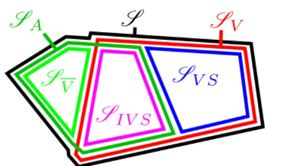
The e-state space S is composed of subspaces that can be identified. The subspace of S gathering all the instant-safe e-states is denoted SA. Conversely, the
com-plementary subspace gathers the e-states violating an e-state constraint; it is denoted SV S (VS for Violation
e-State). As illustrated by Fig. 2, maintaining at each time step σ in SAfor the next time step is not sufficient
to prevent an inevitable e-state constraint violation in the future. As a consequence, a part of SA must never
be reached to guarantee safety.
An e-state leading inevitably to an e-state constraint violation is called an Inevitable Violation e-State (IVS). It is an extension of the notion of Inevitable Collision State (ICS) defined by Fraichard et al. (2004) which denotes a state from which, whatever the sequence of control inputs sent, a collision finally occurs. Once an IVS is reached, the system can be considered as not safe anymore as an e-state constraint violation is going to happen. The space of IVS is a subspace of SA denoted
Fig. 3 Partitioning of the e-state space. To be safe, a system should not be able to reachSV
SIV S. The union of SIV S and SV Sis denoted SV and gathers all the e-states that should be avoided to ensure
safety. The complement of SV in S is denoted SV.
These subspaces are illustrated on Fig. 3. A definition of safety is then
Definition 1 : The safety of a robotic system Σ is
ensured at the control level if its e-state σ cannot reach
SV.
This definition enlightens the role of the constraints expression to limit the evolution of the system toward dangerous areas.
The last subspace to define in this section regards the space that can be reached by a system. Given an initial e-state σ0, R(σ0) denotes the space of all the
reach-able e-states on an infinite time horizon through all the possible constraint compliant control.
3 Methodology to ensure safety
This section exposes the methodology to ensure safety. The proposed methodology must be carried out offline, upstream from the robotic mission. The equivalent of e-state constraints should be formulated at the control level. Once their validity is ensured, they should either be proved compatible, or the permanent availability of an alternative safe behavior must be ensured on an in-finite time horizon.
3.1 Step 1: Control constraints definition
The controller cannot act directly on the e-state σ; it modifies it indirectly through the control vector u. In-versely, at each time step, by imposing conditions on the e-state, each e-state constraint forbids an area of the control vector space C . Hence, to each e-state con-straint f is associated a control concon-straint F which can be defined as the function returning the space of
admissible control vectors CA(σ), i.e. the control vec-tors leading to an instant-safe e-state at the next time
step. A control constraint can be expressed as a Boolean function returning whether a given control vector be-longs to CA(σ) or not
(S , C )7→B
F : (σ, u) 7→ 1 if u ∈ CA(σ) (7)
0 else.
The control input being discrete, control constraints are defined over discrete time (k ∈ N). As an extension of the notation σ(t) (t ∈ R+), σ(k) (k ∈ N) denotes
the e-state at time step k.
In the example of the 3rdjoint superior position limit,
if the control is done at the velocity kinematic level, a possible control constraint is
FP M,3: (σ(k), ˙q(k + 1)) 7→ (8)
˙
q3(k + 1) −
qM,3− q3(k)
δt ≤ 0.
It can be mentioned that from a practical point of view, the inequalities imposed on the system at each time step in the QP control law structure are an exam-ple of control constraints. At a given time step k, these terms are gathered in
JC(q(k)) ˙q(k + 1) − b(k) ≤ 0. (9)
3.2 Step 2: Validity
In order to ensure safety, the first stage is to check that control constraints are valid.
Definition 2 : Validity. Let σ be an instant-safe
e-state at time step k, a control constraint F is said valid if its satisfaction implies the satisfaction of its associ-ated e-state constraint f at next time step k + 1 and for all time between k and k + 1.
σ∈ SA, k ∈ N, ∀t ∈ [kδt; (k + 1)δt] :
F (σ(k), u(k)) = 1 ⇒ f (σ(t)) = 1.
The validity of constraints is most of the time an as-sumption rather than a formally proved property. For example, constraints at various physical levels (posi-tion, velocity, accelera(posi-tion, etc.) must be converted to the control physical level, which is often done thanks to first order approximations (finite differences). The control being in discrete time, the approximations in-duced by finite differences generate errors between the discrete ideal behavior and the real one. However, it is assumed that the sampling period is appropriately cho-sen to ensure that these errors remain acceptable with respect to the various usual sources of errors (model
approximations, sensors precision, etc.). As a remark, it is always possible to find valid control constraints by reducing their space of admissible control vector CA.
3.3 Step 3: Compatibility
A second stage to ensure safety is to check that the set of control constraints is compatible.
Definition 3 : Compatibility. Given an initial e-state σ0 in SV, a set of p control constraints is compatible if for all e-state σ in R(σ0), there exists u in C such
thatVp
i=1(F (σ, u)) = 1.
The following proposition establishes that validity and compatibility ensure safety.
Proposition 1 : Let σ0 in SV be the e-state of Σ, a robotic system constrained by p e-state constraints. If the p control constraints of Σ are valid and compatible, then safety is ensured.
Proof : Let Σ be a robotic system in an initial (time step 0) e-state σ0 belonging to SV. As the control con-straints are compatible, there exists u in C such that
Vp
i=1(F (σ0, u)) = 1. Thus the control problem is feasi-ble and as all the constraints are valid, σ is an instant-safe e-state at time step 1 and for all time between time steps 0 and 1. This reasoning can be extended by recur-sion for all time steps. As a consequence, σ is main-tained in SA on an infinite time-horizon, which means that it is maintained in SV; as a consequence, it cannot reach SV and safety is ensured.
3.4 Step 4: Design of Alternative Safe Behaviors The study of compatibility between control constraints is complex: an exhaustive method would consist to, given an initial e-state σ0, evaluate all the control
con-straints for all the e-states σ reachable from σ0 to
detect empty intersections between control admissibil-ity spaces CA(σ). Given the diversity of constraints, it
seems vain to look for generic methods to detect in-compatibilities and modify control constraints appro-priately to eradicate them. Moreover, sometimes in-compatibilities cannot be resolved: when variables can-not be measured accurately, or when there is no model available, another method should be used to ensure safety.
A second way to guarantee safety is to ensure the per-manent availability of a sequence of control solutions leading to instant-safe e-states on an infinite time hori-zon. At each time step, it is ensured that the controller will be able at next time step to switch to an infinite
sequence of controls leading to exclusively instant-safe e-states. Similarly to the proof of proposition 1, σ is maintained in SA on an infinite time-horizon, which
means that it is maintained in SV; as a consequence, it cannot reach SV and safety is ensured. This control
sequence is called an Alternative Safe Behavior (ASB -referred as evasive manoeuvres by Parthasarathi et al. (2007)). Dedicated ASBs are exposed in Sect. 4.5 ac-cording to the specifications of the proposed case stud-ies.
3.5 Summary and methodology
To describe the physical system Σ and its constraints in continuous time, the e-state σ is proposed, and the sta-tus of the system with respect to its constraints is given by the e-state constraints. Based on this description, a definition of safety at the control level is proposed: Σ is safe if its e-state σ is not able to reach the forbidden e-states SV. In order to prevent this, the control
con-straints F are defined, and the validity property keeps a link between control constraints in discrete time and e-state constraints in continuous time. To ensure safety, either the compatibility property must be proved for the set of control constraints, or the availability of an Al-ternative Safe Behavior must be ensured on an infinite time horizon.
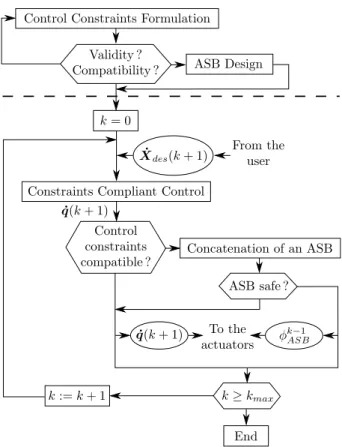
The algorithm presented on Fig. 4 illustrates the fol-lowing methodology:
1. Based on e-state constraints, formulate associated control constraints;
2. Prove validity; 3. Prove compatibility;
4. If step 3 is not possible, either go back to 1 and modify the control constraints expression or define permanently available ASBs. These ASB will then be computed at each time step to ensure that the controller is able to switch at the following time step to an infinite sequence of controls leading to exclu-sively instant-safe e-states.
4 Case studies
To illustrate the approach described previously, three case studies are proposed, based on combinations of the following constraints: {joint position limits - joint veloc-ity limits - joint acceleration limits - collisions avoid-ance} applied to a n-DOFs serial manipulator Σ con-trolled at the velocity kinematic level. The first case study considers compatible constraints with intuitive expressions. The second case study involves constraints
Fig. 4 Safe controller algorithm.The part of the algo-rithm above the dashed line is offline and is concerned with the control problem formulation; the part of the algorithm under the dashed line is online and is concerned with the control problem resolution. From each identified e-state con-straint (physical limit or induced by the mission), a control constraint is formulated offline. If the validity of the con-straints cannot be proved, a new formulation of the control constraints must be expressed. It is always possible to find valid control constraints by reducing their space of admis-sible control vector CA. If the compatibility of the control constraints cannot be proved, a new formulation can be ex-pressed and evaluated, or an ASB must be established. Once this is done, the reactive control loop is launched. At each time step, the controller is fed with operational inputs and solves the control problem thanks to any Constraints Com-pliant Control algorithm. In particular, it can include usual constraints avoidance techniques (e.g. the one of Maciejewski et al (1985)). If the compatibility of the control constraints defined offline could not be proved, an ASB sequence is con-catenated to the desired joint motion: if the resulting behav-ior is not safe, then the first control input of the ASB is sent (represented by φk−1ASB), which safety has been proved at a
previous time step; else, the control solution is sent to the actuators
that must be modified to be proved compatible. The third case study deals with constraints that cannot be proved to be always compatible; as a result, the perma-nent availability of an ASB is required.
4.1 E-state constraints expression
This first section exposes the e-state constraints expres-sions. These expressions describe if, for a given time t in R+, the e-state σ of Σ is instant-safe. The subscripts
mand M denote respectively the minimum (negative
value) and the maximum (positive value) limit of the considered variable.
Joint position limit
fP M : σ(t) 7→ q(t) ≤ qM (10)
fP m: σ(t) 7→ qm≤ q(t) (11)
Joint velocity limit
fV M : σ(t) 7→ ˙q(t) ≤ ˙qM (12)
fV m: σ(t) 7→ ˙qm≤ ˙q(t) (13)
Joint acceleration limit
fAM : σ(t) 7→ ¨q(t) ≤ ¨qM (14)
fAm: σ(t) 7→ ¨qm≤ ¨q(t) (15)
Collisions avoidance A collision is characterized by
Σ\Ω 6= ∅ (16)
where Σ is the system (meant here as the set of all the system points) and Ω is the set of all the obstacles points. The e-state constraint expression is then
fO : σ(t) 7→ ∀A ∈ Σ, GA(q(t)) /∈ Ω (17)
where GA(q) is the geometric model of point A
belong-ing to the robot.
4.2 Case study 1: Joint position limits, Joint velocity limits, Collisions avoidance
This case study involves three constraints: joint position limits, joint velocity limits and collisions avoidance. The following control constraints (assumed to be valid, see Sect. 3.2) are derived from (10) - (15) thanks to finite differences. They are given for a time step k in N.
Joint position limit (ith joint) F P FP M,i:(σ(k), u(k)) 7→ (18) Jc+ i q(k + 1) ≤˙ qM,i− qi(k) δt FP m,i:(σ(k), u(k)) 7→ (19) Jc− i q(k + 1) ≤˙ qi(k) − qm,i δt where Jc+ i = [0, . . . , 0, 1, 0, . . . , 0] (the i th term being 1) and Jc− i = [0, . . . , 0, −1, 0, . . . , 0].
Joint velocity limit (ith joint) F V FV M,i :(σ(k), u(k))7→ Jc+ i q(k + 1) ≤ ˙q˙ M,i (20) FV m,i:(σ(k), u(k))7→ Jc− i q(k + 1) ≤ − ˙q˙ m,i. (21) Collisions avoidance FO FO:(σ(k), u(k)) 7→ (22) JA,B(q(k)) ˙q(k + 1) ≤ dA,B(k) δt
for all pairs of point (A, B), where A belongs to the robot and B to the obstacles; dA,B is the distance
be-tween A and B; JA,B(q(k)) is the (line) Jacobian of
point A along the direction A → B. For practical rea-sons, this infinite set of constraints is reduced to one constraint per segment of the robot (shortest distance). This assumption is frequently made despite its limits in some cases (as shown by Kanehiro et al. (2008)). It is considered sufficient in the present study.
The space of admissible control vectors for control con-straints FP, FV and FO are respectively denoted CAP,
CV
A and CAO.
Validity being assumed (cf. 3.2), the compatibility is checked.
Proposition 2 : The set {FP, FV, FO} is compatible Proof : Let ˙q0 be the null control vector ( ˙q0 = 0) and let σ0 be in SV. For any σ ∈ R(σ0), ˙q(k + 1) = ˙q0 belongs to CP
A, CAV and CAO. As a result, for all σ(k) in
R(σ0), ˙q0 is solution of the control problem and thus FP(σ, ˙q0)V FV(σ, ˙q0)V FO(σ, ˙q0) = 1. ⊓⊔
As all the control constraints are proved to be always compatible, safety is ensured without modification or ASB required.
4.3 Case study 2: Joint position limits, Joint velocity limits, Joint acceleration limits
As in the previous case, this case study involves three constraints but collisions avoidance is replaced by joint acceleration limits. The control constraints for joint po-sition and velocity limits are taken from case study 1 (18) - (21); the control constraint of joint acceleration limit is derived from (14) and (15) thanks to finite dif-ferences (ith joint) FAM,i:(σ(k), u(k)) 7→ (23) Jc+ iq(k + 1) ≤ ¨˙ qM,iδt + ˙qi(k) FAm,i:(σ(k), u(k)) 7→ (24) Jc− i q(k + 1) ≤ −¨˙ qm,iδt − ˙qi(k).
The space of admissible control vectors for control con-straint FA is denoted CAA.
Proposition 3 : The sets of control constraints
gener-ated by {FP, FA} are incompatible.
Proof : Let σ0 be in SV. From σ0, any σV ∈ R(σ0) for which a given joint satisfies
˙q(k) > qM− q(k)
δt − ¨qmδt (25)
is such that FP M,i(σV) and FAm,i(σV) are not com-patible, which traduces that fP M,i and fAm,i cannot be satisfied simultaneously. As there is no assumption or constraint preventing from reaching σV, then FP and
FA are incompatible. ⊓⊔
This incompatibility is illustrated on Fig. 2. It has been locally treated by Decr´e et al. (2009), but as shown in Rubrecht et al. (2010b), the proposed method is tight and can be smoothened by imposing that the joint dis-tance to the joint position limit at next time step should remain superior to the current joint distance needed to decelerate. As a result, a modified expression of FP is
proposed (ith joint) FP M′,i: (σ(k), u(k)) 7→ (26) Jc+ i ˙q(k + 1) ≤ (qM − q(k)) −12(s21− s1)¨qmδt2 (s1+ 1)δt FP m′,i: (σ(k), u(k)) 7→ (27) Jc− i ˙q(k + 1) ≤ (qm− q(k)) −12(s22− s2)¨qMδt2 (s2+ 1)δt with s1= − p−2¨qm(qM − q(k)) ¨ qmδt , (28) s2= p−2¨qM(qm− q(k)) ¨ qMδt . (29)
The choice of (26) and (27) as the joint position limits constraints provoke a small reduction of the reachable positions. Actually, the resolution of ˙q(k + 1) = 0 in (26) induces
qM− q(k) =
−¨qmδt2
8 (30)
which means that the asymptotic value of the joint po-sition according to this constraint is no longer qM but
qM′ = qM −
−q¨mδt2
8 . The order of magnitude of this
reduction is ∼ δt2, which can be considered negligible.
However, it is a reduction of the space of reachable e-state, and all the compatibility studies involving this control constraint must be checked over the joint posi-tion space SP′
A = [qm′; qM′] where qm′ and qM′ are
the vectors of general term respectively qm+q¨Mδt
2
8 and
qM−−¨qmδt
2
8 .
Proposition 4 The set {FP′, FV, FA} is compatible.
Proof Let σ0 be in SV, the current time step k be in N and the current e-state σ(k) be in R(σ0). The design
of (26) and (27) is based on the condition
∆q(k + 1) > dR,dec(k) (31)
where ∆q(k + 1) is the joint distance to the position limit at the next time step and dR,dec(k) is a vector
of upper bounds of the joint distances needed to stop at current time step (cf. Rubrecht et al. (2010b)). This condition implies that the vector of maximum decelera-tion velocity ˙qdec(k + 1) which general term is
˙qdec(k + 1) = ˙q(k) + ¨qmδt if ˙q(k) ≥ −¨qmδt ˙q(k) + ¨qMδt if ˙q(k) ≤ −¨qMδt 0 else (32) belongs to CP′
A (σ). Then, by definition, it belongs to
CA
A(σ). Finally, as it reduces the velocity magnitude, it belongs to CV
A(σ). As a result, for all σ(k) in R(σ0),
˙
qdec is solution of the control problem and thus
FP′(σ, ˙q0)V FV(σ, ˙q0)V FA(σ, ˙q0) = 1. ⊓⊔
This incompatibility between control constraints be-ing resolved, the control constraints are ensured to be always compatible, which ensures safety.
4.4 Case study 3: Joint position limits, Joint velocity limits, Joint acceleration limits, Collisions avoidance This case study involves four constraints, gathering the two previous case studies: joint position limits, joint velocity limits, joint acceleration limits and collisions avoidance. The considered control constraints are (20) - (24), (26) and (27).
Proposition 5 : The sets generated by {FO, FA} are incompatible.
Proof : Let σ0 be in SV. From σ0, any σV ∈ R(σ0) for which
JA,B(q(k)) ˙q(k) >
dA,B(k)
δt − JA,B(q(k))¨qmδt (33)
shows that FO(σ) and FAm(σ) are not compatible, which shows that fO(σ) and fAm(σ) cannot be satisfied si-multaneously. As there is no assumption or constraint preventing from reaching σV, then FO and FA are
in-compatible. ⊓⊔
As mentioned in Rubrecht et al. (2010b), the incom-patibility induced by the simultaneous presence of FO
and FA is complex. Actually, the operational
accelera-tion depends on the robot configuraaccelera-tion (derived from (22)).
¨
which does not enable to rely on any value for the op-erational acceleration capabilities along a trajectory. In the worst cases, these capabilities may fall down to zero, which prevents to take a lower bound on which to rely for the deceleration capabilities estimation. As a result, ensuring compatibility between joint acceleration limits and collisions avoidance seems impossible without an exploration in the neighborhood of the current system e-state, which may turn time-consuming and thus not acceptable in real-time reactive control. In this case, the permanent availability of an Alternative Safe Behavior is required.
4.5 Alternative Safe Behavior
When the control compatibility cannot be proved, the permanent availability of an Alternative Safe Behavior is required, to be triggered in case of critical situation. As mentioned in Sect. 3.4, an ASB is a sequence of control solutions u leading to instant-safe e-states on an infinite time horizon. It must be computed at each time step and the safety of the resulting e-states must be checked, thus it should be fast to compute. To clar-ify the following descriptions, let φ denotes an infinite constraint compliant control input, i.e. an infinite se-quence of controls u satisfying the control constraints at each time step.
4.5.1 Algorithm based on maximum joint deceleration ASB
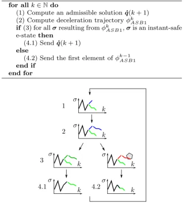
As a preliminary observation, as the environment is as-sumed to be static, once an instant-safe e-state is static (no variation with respect to time), it remains safe until the end of time. Consequently, the first ASB proposed φASB1 is a full deceleration at the joint level. This
de-celeration is the most efficient way to stop the robot: it is fast as no Jacobian has to be recomputed at each time step, and the number of time steps necessary to obtain a static robot is minimized. As the control constraints of joint position, velocity and acceleration limits are compatible, the only remaining constraint to check on all e-states resulting from φASB1is FO, that is an
inter-section between the robot bodies and the environment. The method is detailed on algorithm 1. It is assumed that for k = 0, the initial e-state σ0 belongs to SV.
The algorithm is illustrated on Fig. 5.
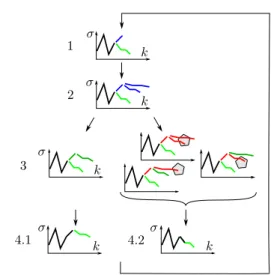
4.5.2 Algorithm based on mixable joint deceleration ASB
As the robot may oscillate between two behaviors (be-tween ˙q(k + 1) issued from the task, and φk−1ASB1
is-Algorithm 1 : Maximum joint deceleration ASB for allk∈ N do
(1) Compute an admissible solution ˙q(k + 1) (2) Compute deceleration trajectory φk
ASB1
if(3) for all σ resulting from φk
ASB1, σ is an instant-safe
e-state then
(4.1) Send ˙q(k + 1) else
(4.2) Send the first element of φk−1ASB1
end if end for
Fig. 5 Algorithm of maximum deceleration based ASB. Blue is for non validated motion, red is for non admissible motion and green for safe motion. 1/ Control solution computation
˙
q(k +1); 2/ ASB1 profile computation φk
ASB1; 3/
Admissibil-ity check; 4.1 (up) and 4.2 (down)/ Send appropriate output
sued from the ASB) a safe but rough behavior is ex-pected from algorithm 1 when moving near obstacles. The problem lies in the maximal deceleration toward the static e-state; when φASB1 is chosen at one time
step, it is likely to be retained until the robot stops. As shown on a simple example in Fig. 6, in most cases there is no available space during φASB1 for another
motion than full deceleration. To have a small margin in the intersection on the control admissibility space, it is proposed to add a prediction φASB2 with reduced
accelerations capabilities. At each time step, both pre-dictions are tested (φASB1 based on ¨qmin/max; φASB2
based on α ¨qmin/max, with α . 1). Once one of these
behavior leads the robot in intersection with the envi-ronment, the robot adopts a φk−1ASB1(maximal decelera-tion). For both behaviors, in case of violation, ¨qmin/max
is applied. If φASB2is violated (in most cases), the
con-trol will then have a margin in the concon-trol admissibility space during its deceleration, where another behavior can be inserted.
The method proposed by Faverjon and Tournassoud (1987) enables to illustrate this approach. This method is referred as the Smooth Avoidance Technique (SAT). Briefly, this method limits the operational velocity of each point of the robot bodies that gets close to an
Fig. 6 Comparative behaviors of robots trying to reach a keypoint (star) behind a wall. On the right, the schemes are representations of the e-states projected on the joint space of the 2nd DOF of the system during 3 time steps. Top:
max-imum joint deceleration (ASB1). The motion of the robot is decomposed in three parts. Black path: the motion is com-puted through the control law, and at each time step the controller concatenates the control vector to be sent with a full deceleration, to check if a collision occurs and decide if the control vector should be sent or not. Red dashed path: a collision with the predicted full deceleration being detected, it is applied before sending the control law computed input; during the ASB deceleration, only the full deceleration control solution is admissible (top right). However, when the robot stops, it is close to the obstacle. Blue path: once near the ob-stacles, the controller oscillates between the control law solu-tions and ASB. Bottom: mixable joint deceleration (ASB1 & ASB2). As in the scheme at the top, the motion of the robot is decomposed in three parts. Black path: control law based motion; it is shorter than the upper one, because deceleration predictions are based on under-estimated capabilities. Red dashed path: the ASB is done with maximal deceleration ca-pabilities, but as it has been triggered before, the control law solutions can be chosen in a small (but not reduced to a point) interval (bottom right). Black path on the green curve: as a result, the robot progression toward the wall can be damped by a smooth path constraint. Green curve: representation of the smooth path trajectory
obstacle. The velocity limitation is done through an in-equality constraint in the QP framework ((2) and (3)). This limitation involves 2 parameters
˙
d = −ad − ds di− ds
for d ≤ di (35)
where ˙d is the temporal derivative of the distance d between the robot point and the obstacle, a is a positive coefficient for adjusting convergence speed, ds is the
security distance and di is the distance influence, i.e.
the distance under which the constraint is activated.
The control constraint associated to (35) is
FC: (σ(k), u(k)) 7→ (36)
JAq(k) ≤ −a˙ dA,B(k) − ds
di− ds
for dA,B(k) ≤ di.
Including the expression of this control constraint at a given time step does not necessarily yield a feasible control problem. However, it is acceptable to violate it as it does not involve security but rather a desired be-havior. Checking the compatibility at each time step is not trivial: knowing if a set of linear constraint is com-patible may require the resolution of the associated lin-ear system. An approximate answer is given by check-ing whether the configuration of maximum deceleration is admissible. It is not a requirement for compatibility (there may be cases for which this configuration is not admissible whereas the constraints are compatible) but it is a sufficient condition. As a result, at each time step the compatibility between the SAT control constraint and the other constraints is checked: if the SAT is not compatible, it is not considered.
The final method is detailed on algorithm 2. As for algorithm 1, it is assumed that for k = 0, the initial e-state σ0 belongs to SV.
Algorithm 2 : Mixable joint deceleration ASB for allk∈ N do
Control constraints: {FP, FV, FA, FO, FC}
if Vpi=1(F (σ, ˙qdec(k + 1))) 6= 1 then Control constraints: {FP, FV, FA, FO}
end if
(1) Compute an admissible solution ˙q(k + 1) (2) Compute deceleration trajectories φk
ASB1, φkASB2
if (3) for all σ1 resulting from φkASB1, σ1 is a safe
e-state AND for all σ2resulting from φkASB2, σ2is a safe
e-state then
(4.1) Send ˙q(k + 1) else
(4.2) Send the first element of φk−1ASB1
end if end for
The algorithm is illustrated on Fig. 7.
5 Results
The following part details the results obtained with a 6-DOF manipulator. The results are composed of 3 ex-periments showing:
– the safe behavior obtained thanks to the resolution of the joint constraints compatibility;
– the safe behavior obtained thanks to the resolution of the joint constraints compatibility and the max-imum joint deceleration ASB;
Fig. 7 Algorithm of mixable deceleration based ASB. Blue is for non validated motion, red is for non admissible motion and green for safe motion. 1/ Control solution computation
˙
q(k + 1); 2/ ASB1 (φk
ASB1) and ASB2 (φ k
ASB2) profile
com-putation; 3/ Admissibility check; 4.1 (up) and 4.2 (down)/ Send appropriate output
– the safe behavior obtained thanks to the resolution of the joint constraints compatibility and the mix-able joint deceleration ASB with the SAT.
5.1 Experiments presentation
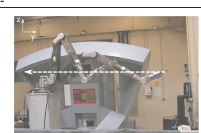
The experiments were performed in a facility of the French Alternative Energies and Atomic Energy Com-mission (CEA), a government-funded technological re-search organization. The 6-DOF arm used in these ex-periments is a 100daN advanced remote hydraulic ma-nipulator with force feedback capabilities, the Maestro (David et al. 2007), designed by CEA and transferred to Cybernetix2. It is usually used in various applica-tions where remote handling with high strength and dexterity are needed, e.g. in nuclear or offshore hostile environments.
5.1.1 Experimental equipment
The robot’s controller uses a generic hard real-time ap-plication, TAO2000 (Gicquel et al. 2001), developed by CEA for Computer Aided Teleoperation Systems (tele-operators) and coming from its experience for objects remote manipulation in hazardous environment. It can address both masters and slaves robots, whatever their kinematics and actuation technologies, providing them a whole generic set of useful features with nearly no specific development. This application provides, via a
2 http://www.cybernetix.fr/Hydraulic-arms
Fig. 8 Teleoperated Maestro operating in front of the tunnel boring machine cutting wheel mockup
standard Ethernet link, a high level communication in-terface to control the robot and a low level real-time tuning and spying interface.
The Maestro works in front of a tunnel boring machine cutting wheel mock-up (Fig. 8). At each time step, the operational input sent is a desired velocity issued from a 3-DOF desired point (position only, no orientation). It induces a Degree Of Redundancy (DOR) of 3.
5.1.2 Initial assumptions versus experimental conditions
Despite the work carried out on safety, the assumptions enounced in Sect. 2 induce approximations which may provoke minor incompatibilities. These incompatibili-ties are localized and do not have a big impact on the robot behavior: as shown on the following results, the envelope needed to absorb them could be small with respect to what would be needed without the compat-ibility study. However, at the control level, an incom-patibility provokes the impossibility to solve the prob-lem. For practical reasons, the occurring incompatibil-ities are denied at the control level: for example, if the current position of the joint parameter q3(k) is inferior
to the artificial minimum joint position qart
m,3, then the
inferior joint position limit is taken as the minimum between the current joint position and theoretical min-imum joint position: qm,3 gets min(q3(k), qartm,3).
From a practical point of view, the envelopes around the joint position limits ejand around the environment
ecare unknown from the controller and considered as an
origin offset: for example, the controller considers that a collision occurs if the distance between the robot and the environment is lower than ec.
Fig. 9 Views of the robot in initial position (extended) and at t = 5.0s (fold up). The white arrow is the constant opera-tional desired velocity from t = 0.0 s to t = 5.0 s
5.2 Safe behavior with compatible constraints
This first experiment3illustrates the behavior of a
multi-body robot subject to control constraints modified to become compatible.
Task presentation. The robot is subject to a brutal
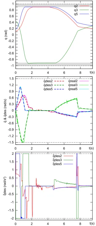
fold up from a configuration of extended robot to a configuration in which the robot has reached its joint position limits (Fig. 9). During a first period (5.0 s), the desired operational velocities are maintained con-stant and maximum toward a point at the left infinite; then, the desired operational velocity brings back the robot toward the initial Cartesian point at lower veloc-ity (the aim is to check that the deceleration toward the joint position limit is safe). The considered e-state constraints are joint position, velocity and acceleration limits ((10) - (15)). For the sake of clarity, the e-state constraints limits are the same for each joint: respec-tively ±1.0 rad, ±1.5 rad/s, ±2.0 rad/s2. The
accel-eration limits have been taken voluntarily low (lower than the robot actual capabilities) in order to better il-lustrate the results. For this particular experiment, the trajectory is considered in a (z,y)-plane (2 DOF desired velocity) and only 3 DOFs are used (see Fig. 9), which brings the DOR to 1.
Control law. The control constraints used to enforce
the considered e-state constraints are FV, FA and FP′
(respectively (20), (21), (23), (24), (26) and (27)). The control problem is expressed as a QP, and the solver is an efficient open source algorithm4.
Given the limits of the robot, the joint position over-shoot could reach 0.56 rad without the proposed method-ology (by taking (18) and (19) as the joint position
3 http://www.isir.upmc.fr/UserFiles/File/...
VpadoiS/Medias/JointPosLim.avi
4 QuadProg++: http://sourceforge.net/projects/quadprog/
control constraints for example). As a benefit of our approach, the envelope retained on joint position limits for this experiment is ej = 0.1 rad.
Results and analysis. The results are presented on Fig.
10. The ˙qdesvalues are the joint velocity sent to the ac-tuators ( ˙q(k + 1)) and ˙qreal are the velocities actually
carried out by the actuators. Only the 3 DOFs con-cerned by the planar trajectory are represented (the other are excluded from the model, so they remain fixed). During the first second, each joint contributes to the operational motion at its best: accelerations are maximal for each joint. Joint 5 is the first to undergo a deceleration (before reaching its maximum velocity) due to the initial proximity to its position limit. Joint 3 reaches its velocity limit for a short time. Joint 2 does not perform high accelerations due to the fact that the operational velocity is sufficiently high thanks to the other joints. At t = 4.0 s, the small motion of joint 2 is induced by a disturbance which, given the system con-figuration, leads to the tracking of the desired Cartesian velocity. At t = 5.0 s, the operational desired velocity is inverted (the robot goes back to its initial operational position), and the robot gets away from its boundaries without any difficulty. At the end of the experiment, (t = 7.5 s), the deceleration is provoked by a reduction of the operational desired velocity; it is not provoked by any constraint. The envelope violation of joint 3 oc-curring at the beginning of the experiment (t = 1.5 s) is attributed to the approximations discussed in Sect. 5.1.2 (especially the exact execution of the desired joint input). However, the envelope is slightly violated, which tends to show that it can reliably be reduced (maximum overshoot is 3.03E−2 rad).
5.3 Safe behavior with ASB
The second experiment5 illustrates the behavior of a
multibody robot subject to incompatible control con-straints; at each time step, the computed control input is sent if a consecutive deceleration toward a static e-state is admissible (see Sect. 4.5).
Task presentation. The robot is subject to various
mo-tions in the cluttered environment of the cutting wheel mock-up (Fig. 8). The desired operational velocity is is-sued from a 3D trajectory involving unreachable points. The considered e-state constraints are joint position, ve-locity and acceleration limits and collisions avoidance ((10) - (15) and (17)). The trajectory involves motions
5 http://www.isir.upmc.fr/UserFiles/File/...
-1 -0.8 -0.6 -0.4 -0.2 0 0.2 0.4 0.6 0.8 1 0 2 4 6 8 q ( ra d ) q2 q3 q5 -2 -1.5 -1 -0.5 0 0.5 1 1.5 2 0 q d e s (r a d /s ) qdes2 qdes3 qdes5 -1.5 -1.2 -0.9 -0.6 -0.3 0 0.3 0.6 0.9 1.2 1.5 0 2 4 6 8 t(s) 2 4 6 8 t(s) q & q d e s (r a d /s) 2 . . .. . . . . . . qdes2 qdes3 qdes5 . . . t(s) qreal2 qreal3 qreal5 . . .
Fig. 10 Position, velocity and acceleration of the joint 2, 3, and 5 during experiment 1. The position is directly measured on the robot, the velocity ˙qdesis the input sent to actuators and ˙qreal is the measured one. The acceleration is computed from ˙qdes. All the variables remain between their limits. The control constraints modification imposes appropriate deceler-ations to satisfy the joint position limits
close to joint position limits. The joint position limits are ±1.0 rad. The joint velocity limits are not reached during this experiment; the joint accelerations limits are set to 1.0 rad/s2. The distances are computed in
real-time using a CAD model of the environment (Fig. 8).
Control law. The control law is similar to the
previ-ous experiment. To deal with incompatible constraints (joint acceleration limits and collisions avoidance), the control uses algorithm 1. To differentiate accelerations due to the trajectory tracking and accelerations issued from ASB1, the acceleration value for prediction and al-ternative behavior is lower than the one retained for the control constraint: 0.9 rad/s2. This modification has no
major impact on the results but makes them clearer. Given the limits of the robot, the joint position over-shoot could reach 0.5 rad without the proposed method-ology. In the same conditions, given the dimensions of the robot, the potential collision without ASB would have required an envelope ∼ 1 m to be avoided. As a benefit of our approach, the envelope retained on joint position limits is ej = 0.1 rad and the envelope around
the environment is ec = 0.1 m.
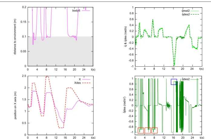
Results and analysis. The results are presented on Fig.
11. The 4 motions getting close to obstacles, easily iden-tifiable at t = 2.0 s, t = 5.0 s, t = 8.0 s and t = 17.0 s on the graph of distance to environment, end-up in the envelope ec. The 3 first motions (t = 2.0 s, t = 5.0 s
and t = 8.0 s) gets close to obstacles with a reasonable velocity, but as there is no compatibility between col-lisions avoidance and acceleration limits, resort to the alternative behavior is needed (red squares). The fourth motion toward obstacles is done at higher speed; the de-celeration begins nearly 1.0 s before the impact (blue square). Finally a motion in the neighborhood of the obstacle generates high frequency oscillations on the ac-celeration (t = 20.0 s). Actually, as the robot remains close to the obstacles, a deceleration at the joint level tends to maintain the robot close to the environment. As a result, oscillations between the trajectory track-ing and the alternative behavior occur. Thanks to the envelope ec taken, safety is preserved.
5.4 Integration of Smooth Avoidance Technique into the mixable joint deceleration ASB
This third experiment6illustrates the possibility to
in-troduce usual collisions avoidance methods into a safe framework for a multibody robot. The resulting behav-ior remains safe and takes full advantage of the avoid-ance method.
Task presentation. The robot is in charge of reaching a
setpoint from which it is separated by an infinite hor-izontal plane (Fig. 12). As in the first experiment, the
6 http://www.isir.upmc.fr/UserFiles/File/...
0 0.5 1 1.5 2 2.5 p o si ti o n o n X a xi s (m ) X Xdes 0 0.05 0.1 0.15 0.2 0 4 8 12 16 20 24 t(s) d ist a n ce t o e n vi ro n m e n t (m) body6 -1 -0.8 -0.6 -0.4 -0.2 0 0.2 0.4 0.6 0.8 1 -1 -0.8 -0.6 -0.4 -0.2 0 0.2 0.4 0.6 0.8 1 qdes2. . qdes2. qreal2. q & q d e s (r a d /s) . . q d e s (r a d /s ) 2 .. 0 4 8 12 16 20 24 t(s) 0 4 8 12 16 20 24 t(s) 0 4 8 12 16 20 24 t(s)
Fig. 11 Results of experiment 2. Left column: shortest distance between body 6 and the environment, desired and real position along Cartesian axis X; right column: desired and real velocity of joint 2, accelerations of joint 2
-0.8 -0.6 -0.4 -0.2 0 0.2 0.4 0.6 0.8 0 2 4 6 8 0 0.05 0.1 0.15 0.2 0 2 4 6 8 d ist a n ce t o e n vi ro n m e n t (m) -1 -0.8 -0.6 -0.4 -0.2 0 0.2 0.4 0.6 0.8 1 0 2 4 6 8 -1.6 -1.4 -1.2 -1 -0.8 -0.6 -0.4 -0.2 0 0 2 4 6 8 p o si ti o n o n Z a xi s (m ) Z t(s) t(s) t(s) t(s) q d e s (r a d /s ) 2 .. q & q d e s (r a d /s) . . qdes2 . . qdes2. qreal2. Zdes body6 I II III
Fig. 13 Results of experiment 3. Left column: shortest distance between body 6 and the environment, desired and real position along Cartesian axis Z; right column: desired and real velocity of joint 2, accelerations of joint 2
Fig. 12 Views of the robot during the trajectory. The red arrows shows the desired operational velocity input along the robot trajectory (green line)
trajectory is considered in a plane (2 DOF desired ve-locity) and only 3 DOFs are used (the same as in Fig. 9), which gets the DOR to 1. The magnitude of the de-sired velocity is maintained constant toward the dede-sired point. At the end of the experiment, a second setpoint is given to get far from the obstacle. The considered e-state constraints are joint position, velocity and ac-celeration limits and collisions avoidance ((10) - (15) and (17)). The trajectory does not involve motion close to joint position limits. The joint velocity limits are not reached along this motion. The joint accelerations lim-its are set to 1.0 rad/s2.
Control law. The control law is based on the one of
ex-periment 2. The approach used to preserve safety in the previous experiment has the severe drawback to gener-ate oscillations on the accelerations when the robot is moving along obstacles. Actually, the control alternates between the trajectory tracking and the alternative be-havior at nearly each time step. As detailed in Sect. 4.5, the control constraint induced by the SAT (36) is added to the set of considered constraints. The fol-lowing values have been used: di = 0.15 m (area I),
ds = 0.07 m (area II) and the envelope around
obsta-cles is ec = 0.05 m (area III). Taking different values
for dsand ec eases the interpretation of the results.
Results and analysis. The results are presented on Fig.
13. As in experiment 2, the arrival on the obstacle causes the maximum overshoot in the area II. The robot never enters the security envelope (area III) as it is managed by the SAT. The distance to obstacle sta-bilizes during the sliding motion (see Fig. 12) until t = 6.0 s when another objective is given to the effector. The transition time can be detected on the acceleration
(blue square), when it switches from 1.0 rad/s2
(decel-eration coming from the alternative behavior) to ap-proximately 0.93 rad/s2. At that time (t = 1.62 s), the
distance to the obstacle is 10.9 cm, and the avoidance method begins to limit the robot motion along direction z. The acceleration is then smooth, the collision man-agement being ensured by the SAT. During the motion along the obstacle (between t = 2.0 s and t = 6.0 s), the velocity of joint 2 contributes to the motion, but the velocity is small as the setpoint is far under the table, increasing the angle between the desired velocity vector and the infinite plane toward orthogonality.
6 Conclusion
The work presented in this paper exposes a method-ology to ensure safety of multibody robots behaviors. Satisfying the constraints at each time step may turn out insufficient because of constraints incompatibilities; as a consequence, to obtain a safe behavior, the control problem can be considered as a problem of constraints expression. The proposed approach enables to study the compatibility of constraints and establishes the link be-tween constraints compatibility and safety. It also pro-poses alternatives if constraints compatibility cannot be established.
Complete case studies illustrate the approach. The constraints expression is modified to ensure compati-bility when possible; if not, the permanent possible re-sort to a safe behavior is ensured. A particular method is developed to take full advantage of the usual avoid-ance techniques while maintaining safety. These works have been applied on a 6-DOF manipulator operating in a cluttered environment. The results obtained con-firm the reliability of the approach and validates the expected performances.
Future works will address new applications and ex-tensions of the proposed methodology. This approach can be applied to other control levels (e.g. torque con-trol) and include other type of constraints related to physical limits (torque limits, jerk limits, power lim-its, etc.) or user specifications (contact persistence, co-manipulation, etc.). The extensions of the presented methodology include the adaptations of the work car-ried out on ICS to IVS. The concept of ICS has gen-erated a significant amount of works in the field of mobile robotics: ICS-checker in the 2D case (Martinez-Gomez et al. 2008), solutions to approximate the ICS set (Parthasarathi et al. 2007), probabilistic approaches (Althoff et al. 2010, Bautin et al. 2010), etc. These works offer many perspectives to increase the use of safe multibody robots.
Acknowledgements This work is involved in the Telemach project; it has been supported by the French National Re-search Agency (ANR), Interactive Systems and Robotics Pro-gram 2007 (PSIROB07).
References
Althoff, D., Althoff, M., Wollherr, D., and Buss, M.
(2010). Probabilistic collision state checker for
crowded environments. In Proceedings of the 2010
IEEE International Conference On Robotics and Au-tomation, pages 1492–1498.
Bautin, A., Martinez-Gomez, L., and Fraichard, T. (2010). Inevitable Collision States: A probabilistic perspective. In Proceedings of the 2010 IEEE
In-ternational Conference On Robotics and Automation,
pages 4022–4027.
Biagiotti, L. and Melchiorri, C. (2008). Trajectory
plan-ning for automatic machines and robots. Springer
Verlag.
Brady, M. (1982). Robot motion: Planning and control. The MIT Press.
David, O., Measson, Y., Bidard, C., Rotinat-Libersa, C., and Russotto, F.-X. (2007). Maestro: a hydraulic manipulator for maintenance and decommissioning application. In Transaction of the European Nuclear
Conference.
Decre, W., Smits, R., Bruyninckx, H., and De Schut-ter, J. (2009). Extending iTaSC to support inequality constraints and non-instantaneous task specification. In Proceedings of the 2009 IEEE International
Con-ference On Robotics and Automation, pages 964–971.
Escande, A., Mansard, N., and Wieber, P.-B. (2010). Fast Resolution of Hierarchized Inverse Kinematics with Inequality Constraints. In Proceedings of the
2010 IEEE International Conference On Robotics and Automation, pages 3733–3738.
Faverjon, B. and Tournassoud, P. (1987). A Local
Based Approach for Path Planning of Manipulators With a High Number of Degrees of Freedom. In
Pro-ceedings of the 1987 IEEE International Conference On Robotics and Automation, pages 1152–1159.
Fox, D., Burgard, W., and Thrun, S. (1997). The dy-namic window approach to collision avoidance. IEEE
Robotics and Automation Magazine, 4(1):23–33.
Fraichard, T. (2007). A short paper about motion
safety. In Proceedings of the 2007 IEEE
Inter-national Conference On Robotics and Automation,
pages 1140–1145.
Fraichard, T. and Asama, H. (2004). Inevitable colli-sion states. A step towards safer robots? Advanced
Robotics, 18(10):1001–1024.
Gicquel, P., Andriot, C., Lauture, F., Measson, Y., and Desbats, P. (2001). TAO2000: a generic control ar-chitecture for advanced computer aided teleoperation systems. In Proceedings of the 9th ANS Topical
Meet-ing on Robotics and Remote Systems.
Guilbert, M., Joly, L., and Wieber, P.-B. (2008). Opti-mization of Complex Robot Applications under Real Physical Limitations. The International Journal of
Robotics Research, 27(5):629–644.
Haddadin, S., Albu-Schffer, A., Eiberger, O., and Hirzinger, G. (2010). New Insights Concerning In-trinsic Joint Elasticity for Safety. In Proceedings of
the 2010 IEEE-RSJ International Conference On In-telligent Robots and Systems, pages 2181–2187.
Ikuta, K., Ishii, H., and Nokata, M. (2003). Safety eval-uation method of design and control for human-care robots. The International Journal of Robotics
Re-search, 22(5):281.
Kanehiro, F., Lamiraux, F., Kanoun, O., Yoshida, E., and Laumond, J.-P. (2008). A local collision avoid-ance method for non-strictly convex polyhedra. In
Proceedings of Robotics: Science and Systems IV,
Zurich, Switzerland.
Khatib, O. (1986). Real-Time Obstacle Avoidance for Manipulators and Mobile Robots. The International
Journal of Robotics Research, 5(1):90–98.
Khatib, O., Yokoi, K., Brock, O., Chang, K., and Casal, A. (2001). Robots in Human Environments. Archives
of Control Sciences, Special Issue on Recent Develop-ments in Robotics, I.11(3-4):123–138.
Kr¨oger, T. (2010). On-Line Trajectory Generation in
Robotic Systems, volume 58 of Springer Tracts in Ad-vanced Robotics. Springer, Berlin, Heidelberg,
Ger-many.
Maciejewski, A. and Klein, C. (1985). Obstacle avoid-ance for kinematically redundant manipulators in dy-namically varying environments. The International
Journal of Robotics Research, 4(3):109–117.
Martinez-Gomez, L. and Fraichard, T. (2008). An ef-ficient and Generic 2D Inevitable Collision State-Checker. In Proceedings of the 2008 IEEE-RSJ
Inter-national Conference On Intelligent Robots and Sys-tems, pages 234–241.
Martinez-Gomez, L. and Fraichard, T. (2009). Collision avoidance in dynamic environments: an ics-based so-lution and its comparative evaluation. In
Proceed-ings of the 2009 IEEE International Conference On Robotics and Automation, pages 100–105.
Park, J. and Khatib, O. (2008). Robot multiple contact control. Robotica, 26(5):667–677.
Parthasarathi, R. and Fraichard, T. (2007). An In-evitable Collision State-Checker for a Car-Like
Inter-national Conference On Robotics and Automation,
pages 3068–3073.
Rubrecht, S., Padois, V., Bidaud, P., and Broissia, M. (2010a). Constraint compliant control for a redun-dant manipulator in a cluttered environment.
Ad-vances in Robot Kinematics: Motion in Man and Ma-chine, pages 367–376.
Rubrecht, S., Padois, V., Bidaud, P., and de Broissia, M. (2010b). Constraints Compliant Control: con-straints compatibility and the displaced configura-tion approach. In Proceedings of the 2010 IEEE-RSJ
International Conference On Intelligent Robots and Systems, pages 677–684.
Zinn, M., Khatib, O., Roth, B., and Salisbury, J. (2004). Playing it safe. IEEE Robotics & Automation