HAL Id: halshs-01131236
https://halshs.archives-ouvertes.fr/halshs-01131236
Preprint submitted on 13 Mar 2015
HAL is a multi-disciplinary open access
archive for the deposit and dissemination of
sci-entific research documents, whether they are
pub-lished or not. The documents may come from
teaching and research institutions in France or
L’archive ouverte pluridisciplinaire HAL, est
destinée au dépôt et à la diffusion de documents
scientifiques de niveau recherche, publiés ou non,
émanant des établissements d’enseignement et de
recherche français ou étrangers, des laboratoires
Long-term care and births timing
Pierre Pestieau, Grégory Ponthière
To cite this version:
WORKING PAPER N° 2015 – 10
Long-term care and births timing
Pierre PESTIEAU
Gregory PONTHIERE
JEL Codes: E13, J13, J14
Keywords: long term care, birth timing, childbearing age, family policy, OLG
models
P
ARIS-JOURDAN
S
CIENCES
E
CONOMIQUES
48, BD JOURDAN – E.N.S. – 75014 PARIS
TÉL. : 33(0) 1 43 13 63 00 – FAX : 33 (0) 1 43 13 63 10
Long-Term Care and Births Timing
Pierre Pestieau
yand Gregory Ponthiere
zMarch 12, 2015
Abstract
Due to the ageing process, the provision of long-term care (LTC) to the dependent elderly has become a major challenge of our epoch. But at the same time, our societies are characterized, since the 1970s, by a signi…cant postponement of births. This paper aims at examining the impact of those demographic trends on the optimal family policy. We develop a four-period OLG model where individuals, who receive children’s informal LTC at the old age, must choose, when being young, how to allocate births along their lifecycle. It is shown that early children provide more LTC to their elderly parents than late children, because of the lower opportunity cost of providing LTC when being retired. In comparison with the social optimum, individuals have, at the laissez-faire, too few children early in their life, and too many later on in their life. The decentralization of the …rst-best optimum requires thus to subsidize early births. We study also the design of the optimal subsidy on early births in a second-best setting. Its level depends on e¢ ciency and equity issues, as well as on its incidence on the long-run population composition and on LTC provision.
Keywords: Long term care, birth timing, childbearing age, family pol-icy, OLG models.
JEL classi…cation codes: E13, J13, J14.
Financial support from the Chaire "Marché des risques et création de valeur" of the FdR/SCOR is gratefully acknowledged.
yUniversity of Liege, CORE, PSE and CEPR.
zUniversity Paris East (ERUDITE) and Paris School of Economics (UMR Paris Jourdan
Sciences Economiques). Address: Ecole Normale Superieure, o¢ ce 201, 48 boulevard Jourdan, 75014 Paris. Contact: [email protected]
1
Introduction
The beginning of the 21st century is characterized by two fundamental demo-graphic trends, which constitute the most recent corollaries of the demodemo-graphic transition started two centuries ago (Lee 2003).
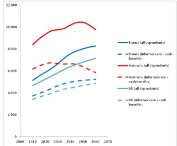
On the one hand, the ageing process raises the proportion of elderly persons in need of long-term care (LTC), i.e. persons who can no longer carry out simple daily activities such as eating, washing, etc. The number of dependent elderly at the European level (EU-27) is expected to grow from about 38 million people in 2010 to about 57 million in 2060 (EU 2012). As shown on Figure 1, the rise in the number of dependent elderly persons is expected to be substantial in most large European economies. The rise of LTC constitutes a major challenge for families, since two thirds of LTC is provided informally (Norton 2000). Forecasts from the EU suggest that a signi…cant part of LTC provision will remain informal in the future. Given the limited development of private LTC insurance markets, this constitutes also a major challenge for policy-makers.1
Figure 1: Number of dependent persons (total / relying on informal care and cash bene…ts), in thousands (source EU 2012)
On the other hand, our societies witness also, since the 1970s, a signi…cant postponement of births (see Gustafsson 2001). Because of various reasons, such as the rise in education, medical advances or cultural norms, individuals tend to have their children later on in their life.2 To illustrate that trend, Figure 2
1On this, see Cremer et al (2012).
2On the various causes of birth postponement, see Cigno and Ermisch (1991) and Happel
shows the rise in the mean age at birth in di¤erent European countries. That rise is substantial: whereas the mean age at birth was below 27 years in France in the late 1970s, it is about 30 years today. The postponement of births has also a signi…cant impact on the dynamics of the age-structure of the economy, and, hence, may a¤ect the …nancial sustainability of systems of intergenerational trade, such as PAYG pensions schemes.
Figure 2: Mean age at birth (source: Human Fertility Database).
Although those two demographic trends may seem, at …rst glance, to be unrelated, those two phenomena are linked through various channels. First of all, as already mentioned, a large volume of LTC services are informal, and provided by the family. Hence the rise of the demand for LTC imposes some pressure on the time constraints faced by other members of the family, such as spouses and children. Given that the time dedicated to LTC cannot be spent on other activities, such as working or educating one’s children, LTC makes time even more scarce for informal care givers. Secondly, when the caregivers are children of the dependent elderly, the age at which caregivers are born has a major impact on the opportunity cost of helping their elderly parents. Clearly, the oldest child of the family is, when his parent becomes dependent, quite old already, and close to retirement. Hence, for the …rst children born in a family, the opportunity cost of helping an elderly parent is lower. On the contrary, younger children are, when their parent becomes dependent, quite young, and are not close to retire, implying a higher opportunity cost of providing LTC.
Whereas those links may appear purely theoretical, empirical studies on informal LTC suggest that informal LTC is far from a marginal phenomenon.
According to recent …gures of the SCAN Foundation (2012), informal caregivers spend, on average, 20.4 hours per week providing care. Moreover, the period during which informal care is given is, on average, equal to 4.6 years. Thus informal LTC really a¤ects time constraints in real life. Regarding the impact of the age of children, recent studies, such as Fontaine et al (2007) showed, on the basis of SHARE data, that the behavior of the children of a dependent parent without spouse is far from symmetric, but, rather, varies with the age of the child and his/her involvement in the labor market. In particular, if younger children are working full time, older children tend to be more involved in the provision of LTC to their elderly parent, even though younger children also participate (in particular when their older brothers and sisters are strongly involved). Thus the age (and, hence, working status) of children providing informal LTC to an elderly parent seems to be an important variable, and this variable is directly related to the fertility choices made by their parents when they were young.
The goal of this paper is precisely to reexamine the formal relations between, on the one hand, the provision of informal LTC by children, and, on the other hand, the timing of births, by paying a particular attention to the impact of LTC on time constraints, and also to the unequal opportunity costs of providing LTC among children of di¤erent ages. More precisely, we would like to examine the conditions under which the timing of birth of children can be used by parents as a kind of insurance device for LTC provision at the old age in an economy where there exist no social insurance system, and where LTC is only provided informally through children.
For that purpose, we develop a 4-period OLG model where individuals be-come dependent at the old age (period 4), and require some help from their children. In order to discuss the fertility timing, we consider a model of lifecycle fertility, where parents can choose to have children in two fertility periods (i.e. periods 2 and 3). We thus consider the joint of decisions of the timing of births and of the provision of LTC to the elderly parents, within a dynamic model of capital accumulation.
Our analysis proceeds in two stages. Our model is …rst used to examine, at the laissez-faire, the relation between birth timing and LTC provision. The question raised is the following: under which conditions do older children provide more or less LTC to their elderly parents, in comparison with younger children? We also characterize the stationary equilibrium of the economy, to examine to what extent our conclusions are robust to the economic development process, which a¤ects the dynamics of the wages and interest rates, and, hence, the opportunity cost of providing informal LTC for children. Then, in a second stage, we propose to characterize the long-run social optimum, and we examine the decentralization of that long-run social optimum by means of appropriate policy instruments. Our question are: what does the optimal family policy look like? Is the birth timing chosen by parents socially optimal in the long-run? Is the postponement of births desirable in times of a rise in LTC?
Anticipating on our results, we …rst show that, at the laissez-faire, early children provide, under mild conditions, more LTC to their elderly parents in comparison to late children, because of a lower opportunity cost of helping their
parents. That tendency is shown to be persistent in the long-run. Then, we characterize the long-run social optimum. We show that individuals have, at the laissez-faire, too few children early in their life, and too many children later on in their life in comparison with the social optimum. The intuition behind that result lies in the fact that, in our model, parents do not perfectly anticipate, when they plan the births of their children, that the chosen birth timing will a¤ect the opportunity costs faced by their children when they will provide LTC 50 or 60 years later, once they will be dependent. As a consequence of this, the decentralization of the social optimum requires subsidies on early births, in such a way as to encourage parents to have children early, so as to minimize the opportunity cost of providing LTC in the future. When considering the second-best problem (and focusing, for simplicity, on an open economy where factor prices are taken as given), we show that the optimal (uniform) subsidy on early births depends not only on standard equity and e¢ ciency concerns, but aims also at internalizing population composition e¤ects, as well as at encouraging the provision of LTC to the dependent parents.
As such, this paper pertains to several branches of the literature. First of all, it complements the existing literature on LTC and family games. That literature already emphasized the crucial role played by the age of children in LTC provision, in particular when the child decides his geographical location (see Konrad et al 2002; Wakabayashi and Horioka 2009). The present paper is not about geographical location choices, but focuses on the di¤erences in the time cost of providing LTC due to the proximity with the retirement period. We also complement other papers on family games and LTC, such as Pezzin et al (2007, 2009), which focus more on strategic motives for LTC provision, without considering endogenous fertility choices. Secondly, our paper is also in line with the literature focusing on fertility as insurance device in case of LTC risk at the old ages (see Cremer et al 2013). Our contribution with respect to that literature is to consider a particular aspect of fertility choices: the timing of births. Thirdly, we also contribute to the literature on optimal public policy under LTC (see Jousten et al 2005; Pestieau and Sato 2006, 2008; Cremer and Pestieau 2010; Cremer and Roeder 2012). Those papers study various aspects of the design of optimal LTC public insurance, but do not consider endogenous fertility. Finally, we also complement the existing literature on childbearing ages and the choice of optimal fertility pro…le in OLG models, such as d’Albis et al (2012), and Pestieau and Ponthiere (2014, 2015). Our contribution with respect to those papers is to highlight the e¤ects of birth timing decisions on the informal provision of LTC in the long-run.
The rest of the paper is organized as follows. The model is presented in Sec-tion 2. The laissez-faire (temporary equilibrium and intertemporal equilibrium) is studied in Section 3. Section 4 characterizes the long-run social optimum. The optimal family policy is derived in Section 5. The second-best optimal policy is studied in Section 6. Section 7 concludes.
2
The model
We consider a four-period OLG model. The duration of each period is normal-ized to 1. Each cohort is a continuum of individuals of size 1. Fertility is at the replacement level, that is, one child per agent.
Period one is childhood. Period 2 is young adulthood, during which individ-uals work, consume, save resources and can have ntchildren. Period 3 is older adulthood, during which individuals work during a fraction of time z 2 ]0; 1[, and enjoy a period of retirement of duration 1 z. During that period, individ-uals consume, save and can have 1 ntchildren. Period 4 is a period of old-age dependency, during which individuals need long term care.
There exist two types of agents, depending on the age of their parent: Type-E agents: children born from young parents (i.e. "early" children) Type-L agents: children born from older parents (i.e."late" children). Within the population of young adults at time t, the proportion of type E agents t is denoted by qt(we have 0 qt 1). The proportion of agents of type L is 1 qt.
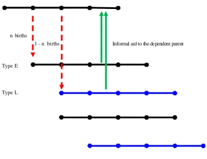
Figure 3 illustrate the coexistence of agents of types E and L; those agents di¤er regarding the age of their parents: while type-E individuals have younger parents (i.e. the age-gap between them and their parents is low), type-L indi-viduals have older parents (i.e. the age-gap between them and their parents is higher). As a consequence of this, those agents will also di¤er in terms of age at the time of providing informal help to their elderly dependent parents. Type-E agents will be older when their parents will fall into dependency and will need LTC. On the contrary, type-L agents will be younger and fully active when their parents will become dependent.
2.1
Preferences
The preferences of a young adult of type i 2 fE; Lg are represented by the following utility function:
u(cit) + v nit + u(dit+1) + v(1 nit) + (ai) + '(biet+2) (1) where ci
t is consumption at the young age, dit+1 denotes consumption in third period. ai is the informal temporal aid given to the parent. It is equal to aE
t+1 for type E and to aL
t for type L. Finally, biet+2 is the expected temporal aid received from children at the old age. As usual, we assume u0( ) > 0; u00( ) < 0; v0( ) > 0; v00( ) < 0; 0( ) > 0; 00( ) < 0; '0( ) > 0 and '00( ) < 0: The parameter 2 [0; 1] captures the extent to which young individuals take into account the impact of their fertility choices on future LTC received at the old age. Full myopia corresponds to the case where = 0, whereas = 1 coincides with the absence of myopia.
n births
1 - n births
Type E
Type L
Informal aid to the dependent parent
Figure 3: Type-E and Type-L agents in the OLG economy
The expected total help received at the old age is the sum of the aid given by each child:
biet+2= nitat+2Ee + (1 nit)aLet+2 (2) We assume here a perfect substitutability between the aid received from the early children and from the late children. The expected levels of temporal aid received from each early child and from each late child, i.e. aEet+2and aLet+2, are likely to di¤er. Actually, since the two types of children will, because of the birth spacing, help their elderly parents at di¤erent points in their life, it is plausible to believe that they will not face the same opportunity cost of helping, and, thus, that they may provide di¤erent amounts of help. Note, however, that the expectations of parents may not fully re‡ect this, and therefore we will consider various kinds of assumptions regarding aEe
t+2 and aLet+2when characterizing the laissez-faire equilibrium.
2.2
Budget constraints
When an agent is of type E, his parent becomes dependent when he is in the third period of his life. Hence, he provides aid to his dependent parent when being an old adult, that is, we have aE
a child costs a fraction in terms of time, the resource constraints are:
wt 1 nEt = cEt + sEt (3)
wet+1z(1 (1 nEt) at+1E ) + Ret+1sEt = dEt+1 (4) where wtis the hourly wage earned at time t, we
t+1is the expected wage rate at time t + 1, while Re
t+1 is equal to one plus the expected interest rate prevailing at time t + 1. The associated intertemporal budget constraint is:
wt 1 nEt + wt+1e z(1 (1 nEt) aEt+1) Re t+1 = cEt + d E t+1 Re t+1 (5) When an agent is of type L, his parent becomes dependent when he is in the second period of his life. Hence, he provides aid to his dependent parent when being a young adult, that is, we have aLt > 0 and aLt+1= 0. Hence, the resource constraints are:
wt(1 nLt aLt) = cLt + sLt (6)
wt+1e z 1 (1 nLt) + Ret+1sLt = dLt+1 (7)
The unique di¤erence between the two sets of budget constraints lies in the mo-ment of life at which children help their elderly parents. In the hypothetical case where there was no help (i.e. aEt+1= aLt = 0), the two sets of budget constraints would be the same across types E and L. The associated intertemporal budget constraint is: wt(1 nLt aLt) +w e t+1z 1 (1 nLt) Re t+1 = cLt + d L t+1 Re t+1 (8) From those constraints, it is obvious that the two types of children do not face the same opportunity cost of helping their dependent parents. Given that early children are close to retirement at the time of helping their dependent parents, they face a lower opportunity cost; on the contrary, late children are at the beginning of their career at the time of helping their parents. Hence, the labor earnings that they must give up to help their parents are larger.
2.3
Production
The production process involves capital Ktand labour Lt, and exhibits constant returns to scale:
Yt= F (Kt; Lt) (9)
The total labor force is made of young and old adults of types E and L:
Lt = qt 1 nEt + (1 qt) 1 nLt aLt
Hence the production process can be written as:
Yt= F (Kt; Lt) (11)
For simplicity, it is assumed that there is full depreciation of capital after one period of use. Hence capital accumulates according to the law:
Kt+1= qtsEt + (1 qt)sLt (12)
As usual, factors are paid at their marginal productivity:
wt = FL(Kt; Lt) (13)
Rt = FK(Kt; Lt) (14)
where wtis the wage rate and Rtequals 1 plus the interest rate. The resource constraint of the economy is:
F (Kt; Lt) = qtcEt + (1 qt)cLt + qt 1dEt + (1 qt 1)dLt + Kt+1
3
The laissez-faire
Let us now consider how individuals of the two types will make their decisions in terms of consumption, fertility and parental help. For that purpose, we will …rst consider the temporary equilibrium, which is a situation where each agent maximizes his utility, conditionally on his beliefs regarding future production factor prices (i.e. we
t+1and Ret+1) and conditionally on his beliefs regarding the future help received from the children born early and late (i.e. aEe
t+2 and aLet+2). For the sake of simpli…cation, we will assume, in the rest of this section, that all agents, whatever these are of type E or L, formulate exactly the same beliefs regarding future factor prices and future help received at the old age.
3.1
Temporary equilibrium
Conditionally on their anticipations, individuals of type E solve the following problem: max cE t;dEt+1nEt;aEt+1 u(cEt) + v nEt + u(dEt+1) + v 1 nEt + (at+1E ) + '(nEtaEet+2+ (1 nEt)aLet+2) s.t. wt 1 nEt + we t+1z(1 (1 nEt) aEt+1) Re t+1 = cEt + d E t+1 Re t+1 First-order conditions (FOCs) yield:
u0(cEt) = Ret+1u0(dEt+1) (15) v0 nEt v0 1 nEt + '0(bt+2Ee) aEet+2 aLet+2 = u0(cEt) wt wt+1e z Re t+1 (16) 0(aE t+1) = u0(cEt) we t+1z Re t+1 (17)
The …rst condition in those FOCs is the standard Euler equation, relating present and future consumption. The second condition characterizes the optimal birth timing. It says that the birth timing is optimally chosen when the marginal welfare gain from increasing the number of early births (LHS of the condition, which is decreasing in nE
t) is exactly equal to the marginal welfare loss from increasing early births (RHS of the condition). Note that the LHS of that condition depends on the di¤erence in terms of the expected LTC received at the old age, depending on the type of child (third term of the LHS). When parents anticipate equal help from early and late children, i.e. aEe
t+2= aLet+2, that term vanishes. If, on the contrary, parents expect to receive more help from their early children, i.e. aEe
t+2 > aLet+2, this increases the marginal welfare gain from having early children ceteris paribus. Hence, for an equal RHS, this leads to a rise in the optimal level of early children nE
t. Inversely, the beliefs aEet+2< aLet+2 reduces the marginal welfare from from having early children, inviting, ceteris paribus, later births (i.e. a smaller nEt). The last FOC characterizes the optimal level of aid provided to the parent. In case of early children, the marginal welfare loss of helping their elderly parent (RHS) is increasing with the retirement age z. Later retirement raises the opportunity cost of helping the elderly.
Individuals of type L solve the following problem: max cL t;dLt+1nLt;aLt u(cLt) + v nLt + u(dLt+1) + v 1 nLt + (atL) + '(nLtaEet+2+ (1 nLt)aLet+2) s.t. wt(1 nLt aLt) + we t+1z 1 (1 nLt) Re t+1 = cLt + d L t+1 Re t+1 FOCs are: u0(cL t) = Ret+1u0(dLt+1) (18) v0 nLt v0 1 nLt + '0(bt+2Le ) aEet+2 aLet+2 = u0(cLt) wt w e t+1z Re t+1 (19) 0(aL t) = u0(cLt)wt (20)
The comparison of the FOCs for the two types of young individuals reveals several things. First, the slope of the consumption pro…le is the same across agents; but the levels of the consumption pro…les can vary across types. Sec-ond, the condition for optimal fertility timing is the same across agents. Hence, given that those agents face the same market prices, the unique di¤erence in birth timing will come from di¤erences in the consumption pro…les. Individu-als with larger consumption at the young age exhibit a lower marginal utility of consumption, which reduces the marginal welfare loss associated with early births (RHS), which encourages advancing births. On the contrary, individuals with a lower consumption at the young age exhibit a larger marginal welfare loss of early births, which encourages birth postponement. Thirdly, the RHS of the condition for optimal help to the elderly parent is also di¤erent from its counterpart for type-E agents. Under the assumption w
e t+1z
Re
t+1 < wt, late children
loss from helping their parents. As shown below, the lower opportunity cost of helping the elderly explains why early children provide, at the laissez-faire, more LTC than late children.
Proposition 1 Given the anticipated levels of future production factor prices we
t+1 and Ret+1, as well as the anticipated levels of future LTC received from the children aEe
t+2and aLet+2, the temporary equilibrium is a vector cEt; dEt+1; nEt; aEt+1; cLt; dLt+1; nLt; aLt; wt satisfying the conditions:
u0(cEt) = Ret+1u0(dEt+1) v0 nEt v0 1 nEt + '0(bt+2Ee) aEet+2 aLet+2 = u0(cEt) wt wt+1e z Re t+1 0(aE t+1) = u0(cEt) wet+1z Re t+1 u0(cLt) = Ret+1u0(dLt+1) v0 nLt v0 1 nLt + '0(bt+2Le ) aEet+2 aLet+2 = u0(cLt) wt w e t+1z Re t+1 0(aL t) = u0(cLt)wt wt = FL(Kt; Lt)
Under the assumption w
e t+1z
Re
t+1 < wt, individuals of type E provide, in
compar-ison with type-L individuals, a larger amount of LTC to their elderly parents, they consume also more and have more early children than type-L individuals:
aEt+1 > aLt cEt > cLt dEt+1 > dLt+1
nEt > nLt
Proof. The …rst part of the proposition is obtained from the FOCs of the problems faced by individuals of types E and L. Regarding the second part of the proposition, this can be obtained by considering the following three cases:
Case 1: cE
t = cLt = ct. Then dEt+1 = dLt+1 = dt+1 from the FOCs for optimal savings and nE
t = nLt from the FOCs for optimal fertility. Hence, from the FOC for aid, we have:
0(aE t+1) = u0(ct) we t+1z Re t+1 0(aL t) = u0(ct)wt Substituting for u0(ct), we have:
0(aE t+1) = 0(aLt) we t+1z wtRe t+1 =) a E t+1= 0 1 0(aLt) we t+1z wtRe t+1
Under cEt = cLt = ct, dEt+1 = dLt+1 = dt+1 and nEt = nLt, we obtain, from the comparison of the budget constraints of the two types, that:
aEt+1= Re t+1wt we t+1z aLt
Collecting those things, we obtain, by transitivity of equality: 0 1 0(aL t) we t+1z wtRe t+1 = aLt R e t+1wt we t+1z
which is a contradiction. Indeed, taking the transform 0( ) on both sides, we obtain: 0(aL t) we t+1z wtRet+1 = 0 aLt R e t+1wt we t+1z which is false except when R
e t+1wt
we
t+1z = 1. Hence this case cannot arise.
Case 2: cEt < cLt. Then dEt+1 < dLt+1 and nEt < nLt. From the FOC for aid, it seems that two subcases can arise: either aEt+1> aLt or aEt+1 aLt. But further analysis shows that only the …rst subcase is possible. To show this, rewrite the two budget constraints as follows:
wt+w e t+1z Re t+1 wt nEt +w e t+1z( (1 nEt)) Re t+1 wet+1za E t+1 Re t+1 = cEt + d E t+1 Re t+1 wt+ wet+1z Re t+1 wt nLt + we t+1z (1 nLt) Re t+1 ! wtaLt = cLt + dLt+1 Re t+1 Suppose that cE
t < cLt and aEt+1 aLt. Then the RHS of the second condition is higher than the RHS of the …rst condition. On the LHS, the …rst two terms are identical across conditions. Given w
e t+1z
Re
t+1 < wt
and nE
t < nLt, the term in brackets term is higher, in absolute value, in the second condition, implying that more is subtracted there. But if aE
t+1 aLt, the last term of the LHS is also larger in absolute value, implying also that more is subtracted there. Hence, the LHS of the second condition is unambiguously lower than the LHS of the …rst condition. But since the RHS must be, under our assumptions, unambiguously larger in the second condition than in the …rst one, a contradiction is reached. Thus the case aEt+1 aLt cannot arise.
Case 3: cE
t > cLt. Then dEt+1> dLt+1 and nEt > nLt. Hence, from the FOC for aid, we obtain that aE
t+1> aLt. Only that case can arise. Proposition 1 states that, provided w
e t+1z
Re
t+1 < wt, individuals born from young
comparison with individuals born from older parents. This result is obtained from the simple fact that early children are older at the time their parents become dependent, and, hence, face a lower opportunity cost of helping them, in comparison to late children. Hence they provide a larger amount of informal LTC.
That result can be related to the existing empirical literature on LTC in-formal provision. Clearly, if we compare the aid provided by two children of the same parent, i.e. aE
t and aLt, we obtain that, under wRttz < wt or
z Rt < 1,
the elderly dependent parent will receive more help from his older children. That theoretical prediction is consistent with the empirical literature on infor-mal LTC provision, which shows that the amount of inforinfor-mal care provided by older children tends to exceed the amount of care provided by younger children when younger children are still working full time whereas older children are not (Fontaine et al 2007).
Note, however, that the size of the inequality in informal help depends on the level of the interest rate, and, more importantly, on the retirement age. A lower retirement age (a lower z) tends to raise inequalities in informal LTC provided between early and late children. Indeed, in that case, the opportunity cost of providing LTC to the dependent parent is much lower for early children in comparison with late children. On the contrary, if z is close to 1, the inequality becomes less sizeable.
Finally, it should be stressed that the di¤erences in the behavior of the two types of agents concern not only the LTC provision, but, also the fertility timing. As stated in Proposition 1, early children tend to have a larger proportion of children born early in life, whereas late children tend to have a larger proportion of children born later on in life. Those results come merely from the di¤erent time constraints faced by the two types of agents. Type-E children must provide LTC to their elderly parents when they are mature, and this leaves them plenty of time to have more children when they are younger. On the contrary, type-L children must provide LTC to their parents when they are young adults, and this encourages them to postpone births later on in their life.
3.2
Intertemporal equilibrium
Up to now, we focused on the temporary equilibrium of the economy. Note that whether early children tend to provide a larger informal help than late children depends signi…cantly on the relative levels of wages and interest rates. However, those factor prices are likely to evolve over time. Hence it makes sense to study the intertemporal equilibrium of the economy, to see how the relative levels of factor prices will evolve over time. In this section, we will characterize the intertemporal equilibrium with perfect foresight.
The intertemporal equilibrium with perfect foresight is a sequence of tem-porary equilibria for a given initial capital stock K0, sequence satisfying the following capital accumulation equation:
as well as the conditions:
wt+1e = wt+1= FL(Kt+1; Lt+1) (22)
Ret+1 = Rt+1= FK(Kt+1; Lt+1) (23)
aEet+2 = aEt+2 (24)
aLet+2 = aLt+2 (25)
At intertemporal equilibrium, the labor market clears:
Lt= qt 1 n E t + (1 qt) 1 nLt aLt +qt 1z(1 aE t (1 nEt 1)) + (1 qt 1)z 1 (1 nLt 1) (26) as well as the market for goods:
F (K; Lt) = qtcEt + (1 qt)cLt + qt 1dEt + (1 qt 1)dLt + Kt+1 (27) At the intertemporal equilibrium, the FOCs relative to individuals’utility maximization problems are also satis…ed:
u0(cEt) = Rt+1u0(dEt+1) v0 nEt v0 1 nEt + '0(bt+2E ) aEt+2 aLt+2 = u0(cEt) wt wt+1z Rt+1 0(aE t+1) = u0(cEt) wt+1z Rt+1 u0(cLt) = Rt+1u0(dLt+1) v0 nLt v0 1 nLt + '0(bt+2L ) aEt+2 aLt+2 = u0(cLt) wt wt+1z Rt+1 0(aL t) = u0(cLt)wt
Similarly, …rms maximize their pro…ts, so that the following conditions hold:
wt = FL(Kt; )
Rt = FK(Kt; )
Finally, the proportion of individuals of type E in each cohort follows the dynamic law: qt= qt 1n E t 1+ (1 qt 1)nLt 1 qt 1nE t 1+ (1 qt 1)nLt 1 + qt 2(1 nEt 2) + (1 qt 2)(1 nLt 2) (28)
3.3
Stationary equilibrium
Let us now consider a stationary equilibrium. At the stationary equilibrium, the economy perfectly reproduces itself over time. The capital stock is constant, the composition of the population in the two types is constant, consumptions are
constant over time, and informal care to the dependent parents is also constant over time, meaning that what a child of a given type gives to his dependent parent is exactly equal to the aid that person will receive from a child of the same type as himself at the old age.
At steady-state, the following conditions are satis…ed (time indexes are dropped):
K = qsE+ (1 q)sL
L = q 1 n
E + (1 q) 1 nL aL
+qz(1 aE (1 nE)) + (1 q)z 1 (1 nL)
That condition can be rewritten as:
L = q nL( z ) nE( z ) + aL zaE + 1 nL aL+ z z + znL
The resource constraint of the economy is thus:
F (K; L) = q cE+ dE + (1 q) cL+ dL + K Factors are paid at their marginal productivity:
w = FL K; q nL( z ) nE( z ) + aL zaE + 1 nL aL+ z z + znL
R = FK K; q nL( z ) nE( z ) + aL zaE + 1 nL aL+ z z + znL
Both types of agents maximize their lifetime welfare subject to their in-tertemporal budget constraints:
u0(cE) = Ru0(dE) v0 nE v0 1 nE + '0(nEaE+ (1 nE)aL) aE aL = u0(cE)hw wz R i 0(aE) = u0(cE)wz R u0(cL) = Ru0(dL) v0 nL v0 1 nL + '0(nLaE+ (1 nL)aL) aE aL = u0(cL)hw wz R i 0(aL) = u0(cL)w
Regarding the long-run composition of the population, imposing qt= qt 1= qt 2 in the condition: qt= qt 1nE+ (1 qt 1)nL (qt 1nE+ (1 qt 1)nL) + qt 2(1 nE) + (1 qt 2)(1 nL) yields: q = n L 1 nE+ nL
The following proposition summarizes key features of the stationary equilib-rium in our economy.
Proposition 2 The stationary equilibrium is a vector cE; dE; nE; aE; cL; dL; nL; aL; K; q satisfying the conditions:
u0(cE) = Ru0(dE) v0 nE v0 1 nE + '0(nEaE+ (1 nE)aL) aE aL = u0(cE)w h1 z R i 0(aE) = u0(cE)wz R u0(cL) = Ru0(dL) v0 nL v0 1 nL + '0(nLaE+ (1 nL)aL) aE aL = u0(cL)w h 1 z R i 0(aL) = u0(cL)w K = q w 1 n E cE +(1 q) w 1 nL aL cL q = n L 1 nE+ nL At the stationary equilibrium, and assuming Rz < 1, individuals of type E provide a larger amount of LTC to their elderly parents, in comparison with type-L individuals. They also consume more and have a larger proportion of early births:
aE > aL cE > cL dE > dL nE > nL
Proof. The …rst part of the proposition is obtained from the FOCs of the problems faced by individuals of types E and L. Regarding the second part of the proposition, this can be obtained by the same kind of argument as at the temporary equilibrium. Consider the following three cases:
Case 1: cE= cL. Then dE = dL and nE = nL. Hence, from the FOC for aid, we obtain that aE> aL. Hence, from the FOC for aid, we have:
0(aE) = u0(c)wz R 0(aL t) = u0(ct)wt Substituting for u0(c t), we have: 0(aE) = 0(aL)wz wR =) a E = 0 1 0(aL)wz wR
Under cE = cL = c, dE = dL = d and nE = nL, we obtain, from the comparison of the budget constraints of the two types, that:
aE= Rwt wz a
Collecting those things, we obtain, by transitivity of equality: 0 1 0(aL)z R = a L t R z
which is a contradiction. Indeed, taking the transform 0( ) on both sides, we obtain: 0(aL t) z R = 0 aL t R z
which is false except when Rz = 1. Hence this case cannot arise.
Case 2: cE < cL. Then dE < dL and nE < nL. From the FOC for aid, it seems that two subcases can arise: either aE > aL or aE aL. But further analysis shows that only the …rst subcase is possible. To show this, rewrite the two budget constraints as follows:
w 1 + z R w n E+z(1 nE)) R wz aE R = c E+dE R w 1 + z R w n L+z(1 nL) R wa L = cL+dL R Suppose that cE < cL and aE aL. Then the RHS of the second condi-tion is higher than the RHS of the …rst condicondi-tion. On the LHS, the …rst two terms are identical across conditions. Given Rz < 1 and nE
t < nLt, the term in brackets term is higher, in absolute value, in the second condition, implying that more is subtracted there. But if aE aL, the last term of the LHS is also larger in absolute value, implying also that more is substracted there. Hence, the LHS of the second condition is unambigu-ously lower than the LHS of the …rst condition. But since the RHS must be, under our assumptions, unambiguously larger in the second condition than in the …rst one, a contradiction is reached. Thus the case aE aL cannot arise.
Case 3: cE> cL. Then dE > dL and nE > nL. Hence, from the FOC for aid, we obtain also that aE> aL.
Proposition 2 states that the tendency of early children to provide more LTC to their elderly parent in comparison to late children is not a short-run phenomenon. Actually, in the long-run, we …nd, under the general condition
z
R < 1, the same tendency. Note that, since at the stationary equilibrium the wage rate is constant over time, the relative gap in the opportunity cost of providing LTC to the elderly parents is even larger here that at the temporary equilibrium, where, under capital accumulation, we have wt+1 > wt, which raises the cost of helping the elderly for early children. Thus, the tendency of early children to provide more LTC to their elderly dependent parents is not a temporary tendency, but is even reinforced in the long-run.
4
Long-run social optimum
Let us now characterize the long-run social optimum. For that purpose, we will consider the standard utilitarian social welfare function. The goal of the social planner is here to select consumption, fertility and informal LTC variables, as well as some stock of capital, to maximize the lifetime welfare prevailing at the stationary equilibrium.
The social planning problem of the utilitarian planner di¤ers from the prob-lems faced by agents in several important dimensions. First, the social planner considers the maximization of social welfare in the long run (i.e. at the station-ary equilibrium), and considers thus a time horizon quite di¤erent from the ones faced by individuals. Second, the social planner does not su¤er from myopia, so that is set to 1 in the social planning problem. Besides those classical di¤erences, another, more original di¤erence concerns the fact that the social planner takes into account the impact of fertility choices on the composition of the population in the long-run. In other words, the social planner internalizes compositional externalities related to individual fertility choices.
The problem of the social planner can be written by means of the following Lagrangian: max cE;dE;aE;;nE cL;dL;aL;nL;K nL 1 nE+nL u(cE) + v(nE) + u(dE) + v(1 nE) + ' nEaE+ (1 nE)aL + (aE) +1 n1 nE+nEL u(cL) + v(nL) + u(dL) + v(1 nL) + ' nLaE+ (1 nL)aL + (aL) + " F K;h nL 1 nE+nL nL( z ) nE( z ) + aL zaE + 1 nL aL+ z z + znL i nL 1 nE+nL cE+ dE 1 n E 1 nE+nL cL+ dL K #
FOCs for consumptions are: :
u0(cE) = u0(cL) = u0(dE) = u0(dL) = (29) The social optimum involves thus an equalization of consumption levels across time periods and across types.
The FOC for K is:
FK K; " nL nL( z ) nE( z ) + aL zaE 1 nE+ nL + 1 n L aL+ z z + znL #! = 1 (30)
This condition is the standard Golden Rule of capital accumulation (Phelps 1961), in the case where there is no cohort growth and where there is full depreciation of capital.
The FOCs for aE and aL are: nL 1 nE+ nL '0( )n E+ 0(aE) + 1 nE 1 nE+ nL'0( ) n L = FL(K; ) zn L 1 nE+ nL (31) 1 nE 1 nE+ nL '0( ) (1 n L) + 0(aL) + 1 nE 1 nE+ nL'0( ) n L = FL(K; ) 1 n E 1 nE+ nL (32)
Further simpli…cations yield:
'0( )nE+ 0(aE) + '0( ) 1 nE = u0(c)FL(K; ) z (33) '0( ) nL+ 0(aL) + '0( ) (1 nL) = u0(c)FL(K; ) (34) The LHS is the marginal social welfare gain from helping the elderly parents, whereas the RHS is the marginal social welfare loss from providing LTC. Ob-viously, that loss depends on how large the marginal productivity of labour is. Moreover, the marginal social welfare loss from providing LTC is larger for individuals of type L than for individuals of type E.
The FOCs for nE and nL are: nL (1 nE+ nL)2 u(cE) + v(nE) + u(dE) + v(1 nE) + ' nEaE+ (1 nE)aL + (aE) u(cL) + v(nL) + u(dL) + v(1 nL) + ' nLaE+ (1 nL)aL + (aL) + n L 1 nE+ nL v0(n E) v0(1 nE) + '0( ) aE aL +u0(c)FL(K; ) " nL nL( z ) nE( z ) + aL zaE (1 nE+ nL)2 + nL( z ) 1 nE+ nL # +u0(c) n L (1 nE+ nL)2 c E+ dE nL (1 nE+ nL)2 c L+ dL = 0 (35) and 1 nE (1 nE+ nL)2 u(cE) + v(nE) + u(dE) + v(1 nE) + ' nEaE+ (1 nE)aL + (aE) u(cL) + v(nL) + u(dL) + v(1 nL) + ' nLaE+ (1 nL)aL + (aL) + 1 n E 1 nE+ nL v0(n L) v0(1 nL) + '0( ) aE aL +u0(c)FL(K; ) " (1 nE) nL( z ) nE( z ) + aL zaE (1 nE+ nL)2 + nL( z ) 1 nE+ nL + z # +u0(c) " 1 nE (1 nE+ nL)2 c E+ dE (1 nE) (1 nE+ nL)2 c L+ dL # = 0 (36)
Further simpli…cations yield: v0(nE) v0(1 nE) + '0( ) aE aL = u0(c)FL(K; ) " aL zaE ( z ) (1 nE+ nL) # u(cE) + v(nE) + u(dE) + v(1 nE) + ' nEaE+ (1 nE)aL + (aE) u(cL) + v(nL) + u(dL) + v(1 nL) + ' nLaE+ (1 nL)aL + (aL) (1 nE+ nL) (37)
while the FOC for nL becomes:
v0(nL) v0(1 nL) + '0( ) aE aL = u0(c)FL(K; ) " aL zaE ( z) (1 nE+ nL) # u(cE) + v(nE) + u(dE) + v(1 nE) + ' nEaE+ (1 nE)aL + (aE) u(cL) + v(nL) + u(dL) + v(1 nL) + ' nLaE+ (1 nL)aL + (aL) (1 nE+ nL) (38)
Note that the two conditions have the same RHS. Hence we have: v0(nE) v0(1 nE) + '0 nEaE+ (1 nE)aL aE aL = v0(nL) v0(1 nL) + '0 nLaE+ (1 nL)aL aE aL Denote the function present in the LHS and RHS by (x) v0(x) v0(1 x) + '0 xaE+ (1 x)aL aE aL . We have 0(x) < 0 on the interval [0; 1] for aE 7 aL. Given that the function (x) is strictly monotone, and that it appears on both sides of the above condition, it must be the case that its argument must take the same value on both sides. From which it follows that, at the social optimum, we have equal fertility across types:
nE= nL = n (39)
Hence, the optimal long-run proportion of early children is:
q = n
1 n + n = n (40)
In the light of this, the FOC for n becomes:
v0(n) v0(1 n) + '0 naE+ (1 n)aL aE aL
= u0(c)FL(K; ) (1 z) aL zaE (aE) (aL) (41)
The LHS of that condition is similar to the LHS of the condition for fertility at the laissez-faire. However, the RHS di¤ers …rst by the fact that R = 1 at the
social optimum, and by the addition of two terms: u0(c)FL(K; ) aL zaE
and (aE) (aL) .
Therefore, the FOCs for informal LTC become:
0(aE) = u0(c)FL(K; ) z '0 naE+ (1 n)aL (42)
0(aL) = u0(c)F
L(K; ) '0 naE+ (1 n)aL (43)
The last term of RHS is the same. First term identical up to z. Hence 0(aE) < 0(aL), implying aE > aL. Hence, at the long-run social optimum, early children should provide more help to their elderly parents than late chil-dren. The following proposition summarizes our results.
Proposition 3 The long-run social optimum is a vector cE ; cL ; dE ; dL ; aE ; aL ; nE ; nL ; K ; q such that: cE = cL = dE = dL = c nE = nL = n v0(n ) v0(1 n ) + '0( ) aE aL = u0(c )FL(K ; ) (1 z) a L zaE (aE ) (aL ) FK(K ; ) = 1 0(aE ) = u0(c )FL(K ; ) z '0( ) 0(aL ) = u0(c )F L(K ; ) '0( ) 0(aL ) 0(aE ) = u0(c )FL(K ; ) (1 z) > 0 =) aE > aL q = n
Proof. See above.
At the utilitarian social optimum, early and late children should have the same life in terms of consumption patterns and fertility patterns. The unique di¤erence is that early children should provide a larger LTC than late children. The intuition goes as follows: from the perspective of social welfare, it is better to ask early children to provide more LTC, since the social opportunity cost of helping their elderly parent is lower for them, as long as z < 1. Note that the gap between aE and aL depends on how large the retirement age is. When z is low, the aid gap is large, whereas, when z is close to 1 (i.e. late retirement), the aid gap becomes tiny.
Having characterized the social optimum, let us now compare it with the stationary equilibrium achieved at the laissez-faire. Proposition 3 summarizes our …ndings.
Proposition 4 Comparing the laissez-faire (i) with the social optimum (i ), we obtain:
Ki< Ki when R > 1 prevails at the laissez-faire, whereas Ki> Ki when R < 1 prevails at the laissez-faire.
Under R > 1 at the laissez-faire, we have: aE > aE aL > aL Provided u0(ci)F L(K; ) 1 Rz '0 niaE+ (1 ni)aL aE aL ? u0(c )F L(K ; ) (1 z) aL zaE (aE ) (aL ) '0 n aE + (1 n )aL aE aL we have: nE ? nE nL ? nL
Proof. The result regarding the capital stock is derived from the Golden Rule condition, in comparison with R ? 1 at the laissez-faire. The di¤erence con-cerning the shape of consumption pro…les follows from comparing the FOCs at the social optimum and at the laissez-faire, under R? 1 at the laissez-faire.
Regarding the amount of informal LTC provided to the dependent parent, the FOCs are, at the laissez faire:
0(aE) = u0(cE)F L(K; ) z FK(K; ) 0(aL) = u0(cL)F L(K; ) whereas these are, at the optimum:
0(aE ) = u0(c )F
L(K ; ) z '0 n aE+ (1 n )aL 0(aL ) = u0(c )FL(K ; ) '0 n aE+ (1 n )aL Provided the conditions:
u0(cE)FL(K; ) z
FK(K; ) > u
0(c )FL(K ; ) z '0 n aE+ (1 n )aL u0(cL)FL(K; ) > u0(c )FL(K ; ) '0 n aE+ (1 n )aL hold, we obtain aE > aE and aL > aL.
If we are in underaccumulation at the laissez-faire (R > 1), we obtain that the LHS exceeds the …rst term of the RHS (since c > ci under R > 1). Given that the second term of the RHS is negative, it is clear that, under underac-cumulation, the two strict inequalities are satis…ed, yielding: aE > aE and aL > aL.
Let us now consider fertility. At the laissez-faire, the FOC for ni was: v0 ni v0 1 ni = u0(ci)FL(K; ) h 1 z R i '0 niaE+ (1 ni)aL aE aL
whereas the FOC for the socially optimal ni is: v0(n ) v0(1 n ) = u0(c )FL(K ; ) (1 z) a
L zaE (aE ) (aL )
'0 n aE + (1 n )aL aE aL
The LHS is the same. But the RHS di¤ers. Hence, provided u0(ci)FL(K; ) 1 z R '0 niaE+ (1 ni)aL aE aL ? u0(c )FL(K ; ) (1 z) aL zaE (aE ) (aL ) '0 n aE + (1 n )aL aE aL we have: nE ? nE and nL ? nL.
The social optimum exhibits several important di¤erences in comparison with the laissez-faire. First, it exhibits a di¤erent level of capital, as well as ‡at consumption pro…les, unlike at the laissez-faire. Secondly, and more impor-tantly, the long-run social optimum exhibits a larger proportion of early births in comparison with the laissez-faire, as well as a lower proportion of late births. The underlying intuition goes as follows. The marginal social welfare loss associ-ated to the informal provision of LTC is larger among late children than among early children. But at the laissez-faire, parents do not take this into account when deciding the timing of births. This explains why they tend to make too many late births in comparison with what is socially optimal. Thirdly, another important di¤erence between the laissez-faire and the social optimum concerns the amount of LTC provision. Individuals of both types tend to provide too little LTC to their elderly parents, in comparison with the social optimum. The intuition is here that young individuals do not, when choosing the amount of help, take into account the welfare gains this generates among the dependent elderly. On the contrary, the social planner takes those gains into account, and this leads to a larger amount of informal aid.
5
Decentralization and optimal policy
Let us now examine how the long-run social optimum can be decentralized. For that purpose, we design policy instruments in such a way that individual decisions at the laissez-faire would, under those policy instrument, lead to the social optimum. The following proposition summarizes our results.
Proposition 5 The long-run social optimum can be decentralized by means of the following instruments:
A system of intergenerational transfers allowing the capital stock to reach its optimal level K .
Intra-generational lump-sum transfers allowing the equalization of con-sumption levels across types E and L.
Subsidies on early births E and Lequal to: i = F L(K ; ) aL zaE + (aE ) (aL ) + aE aL '0 n aE + (1 n )aL '0 niaE + (1 ni)aL u0(c )
Subsidies on informal aid to the elderly parents equal to: E = L = '0( )
u0(c )
Proof. Once the Golden Rule capital level is reached, we have FK(K; ) = R = 1, which automatically makes individual consumption pro…les ‡at: ci= di. The lump-sum transfers also guarantee that all consumption levels are equal across types, i.e. cE= cL and dE= dL.
Regarding the subsidies on early births, remind that the FOC for fertility choices becomes, under such a subsidy:
v0 ni v0 1 ni = u0(ci)FL(K; ) 1
z FK(K; )
u0(ci) i '0 niaE+ (1 ni)aL aE aL Given that the goal is to have ni satisfying:
v0(ni) v0(1 ni) = u0(c )FL(K ; ) (1 z) u0(c )FL(K ; ) a
L zaE
(aE ) (aL ) '0( ) aE aL it is easy to see that the decentralization requires:
i = FL(K; ) 1 z FK(K; ) '0 niaE+ (1 ni)aL aE aL u0(ci) u0(c )FL(K ; ) (1 z) u0(c )FL(K ; ) aL zaE (aE ) (aL ) '0( ) aE aL u0(ci)
Given that FK(K; ) = 1 thanks to intergenerational transfers, the formula can be simpli…ed to:
i
= FL(K ; ) aL zaE +
(aE ) (aL ) + '0 n aE + (1 n )aL aE aL
'0 niaE+ (1 ni)aL aE aL u0(c )
If some subsidies to LTC provision bring aE = aE and aL = aL (see below), this formula can be reduced to:
i= FL(K ; ) aL zaE +
(aE ) (aL ) + aE aL '0 n aE + (1 n )aL
'0 niaE + (1 ni)aL u0(c )
Finally, regarding the aid to the parents, the FOCs would become, under a subsidy i: 0(aE) = u0(cE)FL(K; ) z FK(K; ) u0(cE) E 0(aL) = u0(cL)F L(K; ) u0(cL) L Given that the optimal aE and aL satisfy:
0(aE ) = u0(c )F
L(K ; ) z '0( ) 0(aL ) = u0(c )FL(K ; ) '0( ) It is straightforward to deduce, given FK(K; ) = 1:
E = L= '0( ) u0(c )
Proposition 4 states that the decentralization of the long-run social optimum requires to subsidize early births, in such a way as to induce parents to advance births in a way compatible with long-run social welfare maximization. The decentralization of the long-run social optimum also requires some subsidies on the help provided to the elderly parents. The intuition goes as follows. Individuals help their parents at the laissez-faire, but their help is purely driven by their own interests. However, the dependent parents bene…t a lot from the help provided by their children. The social planner takes into account those welfare gains, and subsidize children’s help to an extent that depends on those welfare gains. Note that the health status of the dependent may strongly a¤ect the level of the derivative '0( ). If the health status is so bad that children’s help does not make them better o¤, i.e. '0( ) 0, then the subsidy should be very low. Thus the public subsidy fully internalizes the welfare externalities induced by children’s provision of LTC.
6
The second-best problem
As shown above, the decentralization of the …rst-best social optimum requires various kinds of policy instruments, some of these being hardly available in real life. In this section, we propose to explore the decentralization of the second-best social optimum, that is, under a limited set of available policy instruments. For that purpose, we will consider an economy at the stationary equilibrium, at which q = 1 nnEL+nL and 1 q =
1 nE
1 nE+nL. Moreover, given that our interest
lies mainly on the design of family policy, we will consider here, for the sake of simplicity, that the economy is open, so that wages and interest rates are …xed.3 We will consider three policy instruments: a tax on labour earnings , a demogrant T and a subsidy on early children . The last instrument can be
used by the government to reduce the cost of early children. For the sake of analytical convenience, the cost of children is here de…ned in terms of goods (and not in terms of time, as in the previous sections).
6.1
Laissez faire
Under those policy instruments, parents of types E and L choose savings si, informal LTC ai and fertility ni and 1 ni conditionally on policy instruments , T and . In what follows, we assume complete myopia of agents, namely = 0. This makes the analysis simpler, but it does not change the qualitative nature of results compared to a case of partial myopia (0 < < 1).
Type E’s problem is:
maxsE;nE;aE u w(1 ) sE nE(1 ) + T +u zw(1 )(1 aE) + sE (1 nE) +v(nE) + v(1 nE) + (aE) FOCs are: u0(cE) = u0(dE) (44) u0(cE) (1 ) = v0(nE) v0(1 nE) (45) u0(dE)zw(1 ) = 0(aE) (46)
Consumption is smoothed along the life cycle. The subsidy on early births tends to encourage earlier births. The last FOC concern the informal LTC provided to the elderly.
Type L’s problem is:
maxsL;nL;aL u w(1 )(1 aL) sL nL(1 ) + T +u zw(1 ) + sL (1 nL) +v(nL) + v(1 nL) + (aL) FOCs are: u0(cL) = u0(dL) (47) u0(cL) (1 ) = v0(nL) v0(1 nL) (48) u0(cL)w(1 ) = 0(aL) (49)
Those conditions are similar to the ones of agents of type E, except regarding the marginal cost of providing informal LTC to the dependent parents, which is here larger (given z < 1).
6.2
Second best solution
Let us now consider the second-best social planning problem. Under the pres-ence of instruments , and T , the social planner chooses the optimal levels of savings, fertility and long term care for both types of agents.
The demand functions obtained from the laissez-faire are, for i 2 fE; Lg: si = si( ; ; T )
ni = ni( ; ; T ) ai = ai( ; ; T )
The second-best planning problem can be written as the following Lagrangian:
$ = q[u w(1 ) sE nE(1 ) + T + u wz(1 )(1 aE) + sE (1 nE) +v(nE) + v(1 nE) + (aE) + '(^bE)] +(1 q)[u w(1 )(1 aL) sL nL(1 ) + T + u wz(1 ) + sL (1 nL) +v(nL) + v(1 nL) + (aL) + '(^bL)] + q w + (1 aE)zw + (1 q)(w(1 aL) + zw qnE+ (1 q)(nL) T where ^bi= aEni+ aL(1 n)i and q = nL 1+nL nE.
Using the envelope theorem and the laissez-faire FOCs, we obtain: @$ @si = 0 (50) @$ @aE = q'0(^b E)nE+ (1 q) '0(^bL)nL qzw (51) @$ @aL = (1 q) ' 0(^bL) 1 nL + q'0(^bE)(1 nE) (1 q)w (52) @$ @nE = U E UL+ w aL zaE @q @nE + q'0(^b E)(aE aL) q + (nE nL) @q @nE (53) @$ @nL = U E UL+ w aL+ zaE @q @nL + (1 q) '0(^b L)(aE aL) 1 q + (nE nL) @q @nL (54)
6.3
Earning tax
Let us introduce the following notations (using the expectation operator E): y = w (q + (1 q) (1 aL)) + wz q(1 aE) + (1 q)
Eu0 = q u0(cE) + u0(dE) + (1 q) u0(cL) + u0(dL)
Eu0y = q u0(cE)w + u0(dE)zw(1 aE) + (1 q) u0(cL)w(1 aL) + u0(dL)zw In order to derive the formula for the optimal tax rate , we consider the derivatives of the compensated Lagrangian with respect to that …scal instru-ment. That derivative amounts to the e¤ect of a marginal change of on the
Lagrangian when the change in is compensated by a variation in T , in such a way as to maintain the government’s budget balanced.
Assuming that cross derivatives in compensated terms are negligible (i.e. @ ~nE @ = @ ~nL @ = @~aE @ = @~aL
@ = 0), that derivative can be written as: @ ~$ @ = @$ @ + @$ @Ty = cov(u 0; y) + A w qz@~aE @ + (1 q) @~aL @ (55) where A @~a E @ h q'0(^bE)nE+ (1 q) '0(^bL)nLi +@~a L @ h q'0(^bE)(1 nE) + (1 q) '0(^bL)(1 nL)i and @~ai @ @ai @ + @ai @T @T @ = @ai @ + @ai @Ty
is the e¤ect of a change of on the amount of LTC provided by type-i agents to their elderly parents when that change in is compensated by a variation in the demogrant T in such a way as to maintain the government’s budget balanced.
Equalizing @ ~@$ to 0 and isolating yields the following tax formula:
= cov(u0; y) + A
w h
qz@~@aE + (1 q)@~@aL
i (56)
To interpret that earning tax formula, we can distinguish between three terms. The …rst term of the numerator is an equity term. Given that individuals with higher incomes bene…t from a lower marginal utility of consumption, we have cov(u0; y) < 0, so that this …rst term is positive, and pushes towards a higher earning tax. The second term of the numerator, A, captures the incidence of the earning tax on the provision of informal LTC by children. By taxing labor earnings, the opportunity cost of providing informal LTC to elderly parents is reduced, which is likely to raise the amount of LTC provided. That term pushes towards more taxation of labor. Finally, the denominator of the tax formula is a standard e¢ ciency term, which captures the incidence of the tax on the tax base.
6.4
Family allowances
Let us now derive the formula for the subsidy on early children . For that purpose, we will use the following notations:
nE = qnE+ (1 q)nL
Eu0E = qu0(cE) + (1 q)u0(cL)
In order to derive the formula for the optimal child allowance , we consider, as above, the derivatives of the compensated Lagrangian with respect to that subsidy. That derivative amounts to the e¤ect of a marginal change of on the Lagrangian when the change in is compensated by a variation in T , in such a way as to maintain the government’s budget balanced.
Assuming that cross derivatives in compensated terms are negligible (i.e. @ ~nE @ = @ ~nL @ = @~aE @ = @~aL
@ = 0), and using the FOCs of the laissez-faire, that derivative can be written as:
@ ~$ @ = @$ @ + @$ @TnE= Eu 0 EnE nEEu0E+ B + C D (57) where B UE UL+ (waL zwaE) @q @nE @ ~nE @ + @q @nL @ ~nL @ C (aE aL) q'0(^bE)@ ~n E @ + (1 q) ' 0(^bL)@ ~nL @ D @ ~n E @ q + n E nL @q @nE + @ ~nL @ 1 q + n E nL @q @nL and where: @ ~nE @ @nE @ + @nE @T @T @ = @nE @ + @nE @T nE @ ~nL @ @nL @ + @nL @T @T @ = @nL @ + @nL @T nE
Hence the tax formula for the early births subsidy is: =cov(u0E; nE) + B + C
D (58)
That formula includes four terms. The …rst term of the numerator is the eq-uity term. The intuition behind that term goes as follows. A family allowance on early births is socially desirable if …rst-period consumption and …rst-period births are negatively correlated. Actually, if individuals with lower …rst-period consumption also have more early children, it makes sense, on equity grounds, to subsidize early births, as a way to redistribute resources towards the disadvan-taged individuals.4 The term B at the numerator gives the e¤ect of composition (q) on overall utility and on earning tax revenue. That term re‡ects that the optimal subsidy on early births depends on its incidence on the long-run com-position of the population. If the decentralized population involves a too large proportion of late children from a social perspective, then this justi…es the sub-sidization of early births, as a way to make the population closer to its optimal
4On that equity e¤ect, see Pestieau and Ponthiere (2013), who study, in a static model
with endogenous birth timing, the design of optimal family allowances when parents di¤er in wage levels.
structure in the long-run. The term C re‡ects the incidence of family allowances on the amount of LTC provided by children. In a hypothetical case where the amounts of informal LTC provided by early and late children would be equal, that term would vanish, since a¤ecting the timing of births would then be neu-tral for the provision of LTC. But as early children face a lower opportunity cost of helping their parents, we have aE aL > 0, implying that this term is likely to be positive. Finally, the term D is the standard e¢ ciency term. It is also expected to be positive. Our results are summarized in the following proposition.
Proposition 6 Assuming a small open economy with R = 1, and assuming that the only available instruments are a tax on earnings , a subsidy on early births and a demogrant T , we obtain that, under negligible cross derivatives, the optimal and the optimal are given by:
= cov(u0; y) + A w h qz@~@aE+ (1 q)@~@aL i = cov(u0E; nE) + B + C D where A @~a E @ h q'0(^bE)nE+ (1 q) '0(^bL)nLi +@~a L @ h q'0(^bE)(1 nE) + (1 q) '0(^bL)(1 nL) i B UE UL+ (waL zwaE) @q @nE @ ~nE @ + @q @nL @ ~nL @ C (aE aL) q'0(^bE)@ ~n E @ + (1 q) ' 0(^bL)@ ~nL @ D @ ~n E @ q + n E nL @q @nE + @ ~nL @ 1 q + n E nL @q @nL Proof. See above.
In sum, our analysis of the second-best problem identi…es the various deter-minants of the optimal subsidy on early births. Besides standard equity and e¢ ciency terms, the level of the optimal subsidy on early births depends also on the incidence of that allowance on the composition of the population, as well as on its incidence on the amount of LTC provided to the dependent parents.
7
Conclusions
The rise of LTC and the postponement of births are two key demographic trends of the last 40 years. This paper proposed to analyze, within a dynamic OLG
model with endogenous birth timing and old-age dependency, the formal relation between those two phenomena.
Our results suggest that the timing of birth de…nitely matters for informal LTC provision. Because of their proximity with retirement, early children face a lower opportunity cost of providing LTC to their elderly dependent parents, in comparison with the opportunity cost faced by late children. Thus, even if all children have exactly the same preferences, and the same interest for the health and the well-being of their parent, they will provide di¤erent amounts of informal LTC, simply because they are not at the same moment in their life, and, hence, do not face the same time constraints.
When studying the stationary equilibrium of the economy, it appeared that the gap in terms of opportunity costs of providing informal LTC to the elderly does not vanish over time, but, rather, is a persistent phenomenon. Thus, the development process will not erase that gap: early children still face, in the long-run, lower opportunity costs, and, hence, will still provide more help to their dependent parents.
On the normative side, we showed that, at the utilitarian optimum, it is also the case that early children should provide more LTC than late children. More importantly, the long-run social optimum involves a di¤erent birth timing than the laissez-faire: it is socially desirable, for the sake of long-run social welfare maximization, to increase the proportion of early births, and to reduce the proportion of late births, in comparison with the laissez-faire. Thus, in the context of LTC provision, decentralized fertility choices do not necessarily coincide with what maximizes social interests in the long-run.
From a policy perspective, this study recommends a di¤erentiated …scal treatment of births, depending on the age of parents. Early births should, to some extent, be encouraged, since these allow the society to bene…t from cheap informal LTC provision from children of dependents who are already retired or close to retirement. Thus the optimal …rst-best subsidy on early births is likely to be positive, and its size depends on the extent to which the decentralized composition of the population in the long-run di¤ers from the socially optimal one, and on how much the decentralized provision of LTC di¤ers from the …rst-best one. We also showed that, once we restrict the set of available …scal instruments to a uniform subsidy on early births, a linear earning tax and a demogrant, the optimal subsidy on early births still depends on its incidence in terms of long run population composition and in terms of LTC provision, but re‡ects also the trade-o¤ between e¢ ciency and equity concerns.
Obviously, this paper, by focusing on the link between fertility choices and in-formal LTC provision, left aside some important determinants of fertility choices, in particular regarding the timing of births. As this is well-known in the lit-erature, fertility decisions and education decisions are strongly related, in the sense that more educated persons have, on average children later on in their life. Hence, the present paper does not have the pretension to cover all dimensions of fertility timing choices. On the contrary, it aimed at exploring the link between fertility timing and informal LTC provision at the old age, and showed that having children earlier can be regarded as some form of preventive behavior or