HAL Id: cea-02415661
https://hal-cea.archives-ouvertes.fr/cea-02415661
Submitted on 17 Dec 2019HAL is a multi-disciplinary open access archive for the deposit and dissemination of sci-entific research documents, whether they are pub-lished or not. The documents may come from teaching and research institutions in France or abroad, or from public or private research centers.
L’archive ouverte pluridisciplinaire HAL, est destinée au dépôt et à la diffusion de documents scientifiques de niveau recherche, publiés ou non, émanant des établissements d’enseignement et de recherche français ou étrangers, des laboratoires publics ou privés.
Sensitivity analysis of pounding pounding between
adjacent structures
V. Crozet, I. Politopoulos, M. Yang, J.-M. Martinez, S. Erlicher
To cite this version:
V. Crozet, I. Politopoulos, M. Yang, J.-M. Martinez, S. Erlicher. Sensitivity analysis of pounding pounding between adjacent structures. Earthquake Engineering and Structural Dynamics, Wiley, 2018, 4, pp.219-235. �10.1002/eqe.2949�. �cea-02415661�
SENSITIVITY ANALYSIS OF POUNDING BETWEEN ADJACENT STRUCTURES Crozet V.1, Politopoulos I.1,*,†, Yang M.2, Martinez J.M.1,Erlicher S.3
1
Commissariat à l’énergie Atomique, DEN, DANS, DM2S, Université Paris-Saclay, F-91191 Gif-sur- Yvette, France
2
Centre Scientifique et Technique du Bâtiment, F-77420 Champs-sur-Marne, France
3
Egis Industries, F-93188 Montreuil, France
SUMMARY
This article deals with sensitivity of the response of pounding buildings with respect to structural and earthquake excitation parameters. A comprehensive sensitivity analysis is carried out by means of Monte Carlo simulations of adjacent single degree of freedom impacting oscillators. This sensitivity analysis, based on Sobol’’s method, computes sensitivity indexes which provide a consistent measure of the relative importance of parameters such as the dimensionless main excitation frequency, the mass and frequency ratios of the structures and the coefficient of restitution. Moreover, the influence of nonlinear behavior of the impacting structures is also considered. The consequences of pounding on the structures themselves, are analyzed in terms of maximum force and nonlinear demand amplification compared to the case without pounding. As for the influence of pounding on the floor response spectra, the quantity of interest is the maximum impact impulse. The overall conclusions of this analysis are that the frequency ratio is the most important parameter as far as the maximum force and nonlinear demand are concerned. Regarding the maximum impact impulse, the mass and frequency ratios are, in general, the most influential parameters, the mass ratio being predominant for low frequencies of the oscillator of interest. KEYWORDS: buildings pounding, sensitivity analysis, floor response spectra
1. INTRODUCTION
The interaction between adjacent structures during earthquakes became of interest as researchers gathered evidence of its occurrence over last decades [1-3]. This phenomenon has been source of local damages in buildings as well as in bridges, and in some cases it might be thought that it lead even to failure onset [4, 5]. Moreover, in the case of industrial and power generation facilities, acceleration spikes may influence floor response spectra and thus the response of equipment. Pounding between bridge decks was recorded during Landers and Big Bear 1992 earthquakes resulting in large amplitude, short duration acceleration spikes and compression waves traveling through the decks [6]. Other events for which pounding between buildings was recorded may be found in the literature [7, 8].
These records confirm the experimental conclusions [9-12], that pounding between structures during earthquakes is a source of considerable acceleration amplification in both structures, in the form of high amplitude acceleration spikes. In addition, experimental observations underlined that pounding can significantly modify the displacement response of the impacting structures, especially in the case of notable differences of structures’ masses and resonant frequencies. Nevertheless, the potential damaging effect of pounding is a subject of controversy since
conflictual results, conclusions or statements can be found in both analytical and experimental studies and reports on feedback from past earthquakes [2].
For instance, regarding displacement amplification (i.e. force amplification in the case of linear elastic response of each building) contradictory conclusions are found. Papadrakakis and Mouzakis [9] concluded, on the basis of a shake table test and numerical simulations, that pounding resulted in displacement amplification and reduction of the stiffer and more flexible buildings, respectively. Nonetheless, Jankowski [11] observed, with another experiment, that this conclusion could be challenged if the mass of the more flexible structure is much bigger than that of the more rigid structure.
With respect to impact simulation, several methods amongst the methods used, in general, for impact problems have been considered by various authors. For instance, a classical Lagrange multiplier method has been used in [13], while an impact element based on Hertz contact law was used to model pounding between structures in [14, 15] . This contact law shows peculiarly suitable results when the impact zone behaves elastically and its size is quite limited compared to the size of the impacting bodies [16]. Penalty like methods, such as classical gap elements composed of a spring in parallel with a damper, have also been used [17]. Khatiwada et al. [18] carried out a comparative study between a linear viscoelastic impact element model and a Hertz contact law based model. Comparison of numerical simulation results with experimental recorded displacement amplification of frames, with rather regular shape impacting slabs, showed that the linear viscoelastic impact element provided the most satisfactory results. Difficulties to assess the values of the impact gap element characteristics are inherent to this representation [19]. In an effort to impose the non-penetration condition, a high value of the spring stiffness, compared to the stiffness of the impacting structures, may be considered. This gap spring stiffness may also be considered to account for flexibility that is not represented by the model (e.g. local flexibility, flexibility of higher modes in the case of modal representation of the structures). The role of the damper is to account, in a simplified fashion, for the energy loss during impacts. Its coefficient may be determined as a function of the coefficient of restitution, ε, which is equal to the ratio of the pre-impact to the post-impact relative velocities. Though, commonly, a constant value of ε is considered, experimental results show that it depends on the pre-impact velocity [11].
Regarding the influence of the configurations of the impacting structures, Efraimiadou et al. [20] investigated the consequence of pounding on different combinations of reinforced concrete planar frames. The same authors [21] studied also the effect of sequences of earthquakes on damage indexes. The influence of soil-structure interaction was studied in [22] and [23] by means of simplified lumped mass-spring-dashpot models for the soil. As for the necessary minimum distance between buildings to avoid pounding, [24], taking into account soil-structure interaction, concludes that the recommendations of the International Building Code 2009 on this respect are unconservative.
Nevertheless, despite a rather considerable research in this field, except some special cases (e.g. pounding between slab and columns), there is no consensus regarding the consequences of pounding for the general case of two adjacent structures. In some studies an effort has been made to understand the physics. For instance, [25, 26] focus on two adjacent impacting oscillators or an oscillator impacting with a rigid barrier (either fixed or following the ground motion) submitted to sine waves excitation. These studies highlighted the well-known fact [27] that, for some
excitation frequencies, periodic impacts do not occur and the oscillators do not exhibit a steady state despite the periodicity of the excitation. Dimitrakopoulos et al. [28-30], used dimensional analysis for single degree of freedom (SDOF) oscillators interacting with each other or with a rigid wall while they are subject to pulse like excitation [28, 29] or natural accelerograms [30]. Their dimensionless analysis provides self-similarity of the impacting oscillators’ dimensionless maximum displacements regardless the excitation maximum acceleration. They drew meaningful conclusions on the dimensionless displacement response modification due to pounding depending on the SDOF oscillators’ characteristics in terms of frequency and mass ratios as well as on the oscillators’ constitutive law. It is observed that, in the case of two interacting oscillators under pulse excitation, the maximum dimensionless displacement of the flexible oscillator occurs for an excitation frequency equal to the stiffer oscillator’s frequency. Similarly, amplification of the dimensionless displacement of the stiffer oscillator is observed for excitation frequencies near the flexible oscillator’s frequency, even though its global maximum is located in the vicinity of the frequency of the stiffer oscillator. It is therefore concluded that structures subjected to pounding might be vulnerable to excitations with predominant frequencies quite different from their natural eigenfrequencies. These studies highlight also, the existence of three regions (amplification, deamplification and unsensitivity) when the dimensionless displacement response is plotted as a function of the ratio between the frequency of one oscillator and the frequency of the excitation sine or cosine pulse or the main frequency of the earthquake record.
Nevertheless, the above studies do not apply a systematic method to determine the importance of each parameter. Actually, the results are analyzed by visual inspection of curves of the output parameter as a function of only one or two dimensionless parameters. Hence, it is not easy to identify the most influential parameters. Therefore, in an effort to extend the results of these studies, we carried out a comprehensive sensitivity analysis of the earthquake induced pounding between two SDOF oscillators. The sensitivity analysis consists in analyzing the relation between variabilities of the output and input parameters. Several methods exist to study sensitivity from a local or more global point of view [31]. The global sensitivity analysis applied in this work, Sobol’’s method [32], consists in calculating the contribution of the variations of the input parameters to the variance of the model output. Linear elastic and nonlinear oscillators with constitutive laws being simplified approximations of actual buildings behavior under seismic loading are considered. The consequences of pounding on the structures themselves are analyzed in terms of maximum force and nonlinear displacement demand amplification compared to the case without pounding. In addition, unlike most of the previous studies, this work investigates also the influence of pounding on floor response spectra. To this end, as it will be shown in section 6 the relevant output quantity of interest is the observed maximum impact impulse. 2. MODEL DESCRIPTION
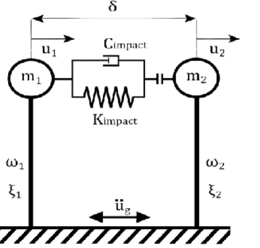
As already mentioned, the simplest model of two impacting oscillators (Figure 1) is considered here for the purpose of the sensitivity analysis. Actually, the number of parameters increases quickly with increasing number of degrees of freedom resulting in higher computational cost and rendering the interpretation of the result more difficult.
A nonlinear gap element composed of a spring in parallel with a viscous damper is employed to model impact. The impact element stiffness,
impact
K ,is chosen to be 100 times the stiffness of the
more rigid oscillator. This is a balance struck between the unilateral condition requirement (zero penetration) and a reasonable time step. Hence, the spring stiffness is not an independent variable for the sensitivity analysis. Actually, as expected, a comprehensive parametric study shows that the dimensionless output of interest exhibits, practically, a similarity of the first kind [33] with respect to the dimensionless impact stiffness (i.e. it tends to a non-zero limit when the dimensionless impact stiffness becomes large). That is, the response quantities of interest do not vary significantly when the value of the impact stiffness changes one or more orders of magnitude as far as it remains much higher than the stiffness of the impacting oscillators. The chosen value of the contact stiffness implies that the characteristic time of impact is about, at least, ten times shorter than the characteristic time of the pre and post impact response of the oscillators. Hence, under these conditions, the quantities of interest (maximum displacement, maximum impact impulse, ductility demand) are not very sensitive to the precise value of the contact stiffness. Of course, modifying the contact stiffness would result in small differences of the pre and post impact conditions and thus in differences of the response time histories. Actually, it is well known that the exact response time history of most impacting systems is practically unpredictable. Nevertheless, the above response quantities of interest do not vary considerably. Moreover, in this study, as explained in the following sections, we are interested in mean output quantities and thus their sensitivity is even smaller. The above conclusions hold for the response quantities of interest of this study but not for the peak accelerations. In fact, the higher the impact stiffness is, the higher the peak acceleration will be.
As for the viscous damper impact
C , it is tuned so as to result in a ratio of post-impact to pre-impact relative velocities of the colliding bodies equal to the coefficient of restitution , which is a varying parameter in this study [34].
2 1 2 1 2 m m m m K
Cimpact impact impact (1)
where
2 2
ln ln impact (2) 2.2. ExcitationRegarding the excitation, it is obvious that its frequency content may play an important role in the pounding problem. Nevertheless, considering in the sensitivity analysis a detailed description and variability of the excitation frequency would have been a very difficult if not unfeasible task. Therefore, in an effort to associate only one frequency parameter to the excitation, artificially generated signals compatible with a Kanai-Tajimi filtered white noise [35] are considered. Furthermore, a high pass filter is also applied to avoid infinite velocity and displacement at zero frequency. It is reminded that the Kanai-Tajimi filter is the frequency response function between input and output acceleration of an oscillator and thus it is characterized by a frequencyeand a
critical damping ratioe. Therefore, the filter frequency e is retained as the excitation frequency
parameter. To limit the number of parameters to deal with, the critical damping ratio is assumed constant, e 0.6, which is a commonly used value to model wide band earthquake signals [36]. It is worth noting that, because of the high filter damping value, the filter frequency is equal neither to the main frequency nor to the Rice frequency, which coincides with the number of zero crossings with the same slope sign within a time unit. Another reason for the choice of this kind of natural records is that a big number of different records are needed for the Monte Carlo based sensitivity analysis to deal with the excitation variability. Clearly, such a big set of consistent natural records does not exist. Moreover, to account for transient excitations, the signals are multiplied by a trapezoidal temporal envelope.
Figure 1. Model of two interacting oscillators 2.3. Constitutive laws of oscillators
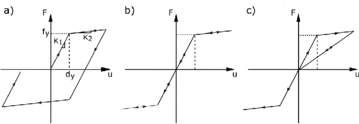
To provide a broad overview of the consequences of pounding on buildings, different constitutive laws for the oscillators are considered. Thus, in addition to linear elastic behavior, three nonlinear constitutive laws which are rough approximations of the nonlinear behavior of some, commonly met, structural systems are considered (Figure 2). In fact, an elastoplastic law with kinematic hardening is used to model the performance of ductile steel structures, whereas, an origin oriented law is applied to approximate the behavior of stiffness degrading concrete structure. Finally a nonlinear elastic behavior is used as an approximation of the response of walls that exhibit uplift at their base because of foundation uplift or because of a full depth crack. It may also be used to approximate the behavior of prestressed unbonded precast joints [37].
In all cases, a low stiffness after nonlinear onset is reached (slopeK2in Figure 2) is assumed. To reduce the number of parameters, throughout this study, the value of the second slope is fixed to 5% of the initial stiffness. As an index of the nonlinearity exhibited by each structure we consider the nonlinear displacement demand: i dimax/dy
, where dimax is the maximum
displacement of oscillator i without pounding and dy is the displacement corresponding to the onset of nonlinear behavior. In the case of an elastoplastic behavior i is the displacement
ductility demand. For each oscillator, the output quantity of interest for the sensitivity analysis will be the ratio of the nonlinear displacement demand when impact occurs to that without impact.
For the results of the sensitivity study to be meaningful, the yield strength (or, equivalently, the yield displacement) should be chosen appropriately. Therefore, to focus on the effect of impacts on the nonlinear displacement demand, it would be desirable that, in the nonlinear case, all oscillators exhibit the same amount of nonlinear demand when impact does not occur. To this end, for each excitation signal and oscillator, the yield strength must be determined through a trial and error iterative procedure. Nevertheless, due to the big number of possible oscillators-excitations combinations considered in the sensitivity study, the computational cost of such an iterative procedure would have been extremely high. Therefore, instead, we determined the yield strength by a force reduction factor, such as the response modification factor(e.g. FEMA 368 [38]) or the behavior factor (Eurocode 8 [39]). Similar to the above regulations, we admit the splitting of the above factors to a part due to redundancy and design overstrength and a part due to ductility capacity (or nonlinear deformation in the general case). Only the part accounting for ductility has
to be considered in the determination of the design strength because the part due to overstrength has been, implicitly, taken into account by modifying the first slope of the simplified bilinear curves shown Figure 2. Then, the displacement corresponding to the onset of nonlinear behavior is set to dy delmax/qy
where delmax corresponds to the maximum displacement undergone by a linear
elastic oscillator and qy is a reduction force coefficient. As shown in Figure3, qy depends on the target nonlinear demand d and on the ratio between the excitation and the oscillators’
frequencies. This frequency dependent evolution of qy is consistent with the philosophy of the aforementioned recommendations. For dimensionless excitation frequencies higher than 1/6, equality of the maximum displacements of the linear and nonlinear responses is assumed. For lower dimensionless frequencies, a smaller reduction factor is considered in order to prevent high
Figure 2. Nonlinear constitutive laws. a) Elasto-plastic. b) Nonlinear elastic. c) Origin oriented.
nonlinear demand. In an effort to obtain, for a given signal and a given oscillator, a nonlinear demand closer to the target one, once a first estimate of dy is obtained by the above procedure, a nonlinear run, without impact, is carried out. In general, the nonlinear demand of this run may be different from the target one and a correction step is applied to adjust dy. That is, we do only the first iteration of the aforementioned trial and error iterative procedure. Throughout this study,
2
d
is assumed.
As already mentioned, the consequences of pounding on the main structure are analyzed in terms of maximum force (or displacement) amplification for the linear elastic oscillators and in terms of nonlinear displacement demand amplification for the nonlinear oscillators. These quantities may be considered as relevant indexes for possible adverse effects of pounding on the structures themselves. In addition, with respect to the response of equipment and components, the effect of pounding on the floor response spectra is addressed in a dedicated section.
3. DIMENSIONAL ANALYSIS MODEL :
To carry out a sensitivity analysis of general validity, it is important to employ dimensionless input and output variables. The choice of the dimensionless products is presented in this section. Let us look at an output quantity of interest, for instance, the maximum displacement max
i
U of oscillator i (i = 1, 2). In the case of elastic linear behavior of both oscillators, according to the above described model, Uimax depends on ten parameters and one function of time: )) ( , , , , , , , , , ( 1 2, 1 2 1 2 max t f A K m m F Ui impact (3)
where 1,2 are the oscillators’ frequencies, 1,2 their critical damping ratios, m1,m2 their
masses, Kimpact the impact stiffness, the coefficient of restitution, the initial gap between the oscillators and A and f(t) are the earthquake acceleration maximum amplitude and normalized time evolution, respectively. Let us repeat several computations with the same set of structural parameters and acceleration amplitude A but different signals f(t) generated, according to the procedure described in the previous section, for the same values of the Kanai-Tajimi filter parameters e and e and the same time envelope. Then, the mean maximum value
max
i
U will no longer depend on the details of each individual signal but on the parameters of the process characterizing the excitation i.e. A,e,e,T where T is the duration of the signal. In order to
obtain an index of the influence of the impact, Umaxi may be normalized with respect to the mean
maximum displacement of the same oscillator when pounding does not occur umaxi .
) , , , , , , , , , , , ( 1 2, 1 2 1 2 max max T A K m m F u U e e impact i i (4)
According to Vachy-Buckingham’s Pi theorem, Equation (4) can be written in a dimensionless form with N-r dimensionless variables where N is the number of the initial variables and r is the rank of the matrix of the dimensions’ exponents of the variables. In the present case 𝑁 = 14 and
𝑟 = 3 (i.e. equal to the number of fundamental dimensions: mass, time and length), thus there are 11 dimensionless parameters. ) , , , , , , , , , ( 1 2 2 2 1 2 1 1 2 max max T A m K m m u U e e e i i i impact i i (5)
Alternatively, the dimensionless gap could also read /uimax.
In the sequel, to reduce the number of varying dimensionless variables for the sensitivity analysis, we assumed fixed values for the dimensionless duration and the critical damping ratios. The critical damping ratio of both oscillators is fixed to 5% and, as already mentioned, the Kanai-Tajimi filter damping ratio is fixed to 60%. Moreover, as already explained in the previous section, a sufficiently stiff impact spring is chosen and thus, the corresponding dimensionless parameter does not enter in the sensitivity analysis. Regarding the gap, the choice 0 has been made. In addition to lower by one the number of varying variables, this choice is motivated by physical reasons also. Actually, if 0, in the Monte-Carlo simulations, cases with impact and cases without impact will occur. This is not a concern in the case the variability of each parameter (e.g. range of values and probability density function) is assumed to be its actual variability and the output is to be interpreted as an index of sensitivity taking into account representative statistics of the system. However, this is not the case here, where we use methods of statistics just as a tool to determine the more influential parameters without any statistical reality. For instance, in this study, contrary to vulnerability studies, considering that the frequency of each oscillator varies uniformly between a minimum and maximum value does not mean that the actual population of buildings subjected to pounding meets this condition. As already mentioned, our goal is to study the sensitivity of a relevant output index of the influence of pounding on the response. Therefore, from this point of view, it is better if only cases where impact occurs are considered and the choice 0 ensures that pounding will always occur. Even more, even if 0 does not necessarily lead always to higher response amplification than
0
, it may be reasonably expected that, in general, in the former case the influence of pounding will be considerable.
Eventually, in the case of linear interacting oscillators the following four varying input dimensionless variables are considered in the sensitivity study:
, , , 1 2 1 2 1 m m m e e (6)
The output variable will be U Umaxi /umaxi as an index of the displacement (or, equivalently force) amplification.
In the case of two nonlinear interacting oscillators, the output variable is the normalized mean nonlinear displacement demand:
np i p i (7) where ip and np i
are the mean nonlinear demands with and without pounding respectively. Two additional variables for oscillator i, the linear limit force f (or the linear limit yi
displacementd )iy and the second slope of the skeleton curves shown in Figure 2 ( i
k2) are involved and thus, two additional dimensionless variables have to be considered for each oscillator with respect to the linear case.
) , , , , , , , , , , , ( 2 2 2 1 2 2 2 1 2 1 1 2 A d m k T A m K m m e i y i i i e e e i i i impact np i p i (8)
The last two dimensionless terms in the r.h.s. of Equation (8) are the hardening ratio and the dimensionless linear limit displacement. As already mentioned in section 2, a fixed value, equal to 0.05, is considered for the hardening ratio. As exposed in the same section, the linear limit displacement is determined so that the nonlinear displacement demand without impact is equal to 2. That means that the dimensionless linear limit displacement is not an independent variable but it is uniquely determined for a given set of the remaining dimensionless variables (the nonlinear displacement demand included). Hence, eventually, the same input varying dimensionless variables as in the linear case are considered for the nonlinear case also.
In both cases, of linear and nonlinear interacting oscillators, the dimensionless maximum impulse
Imp
is considered as a relevant output index of the influence of pounding on the floor response spectra. max max Imp Impulse i i i u m (9)
where Impulsemax is the mean value of the maximum impact impulse:
k t c k F dt max Impulsemax (10)where tk is the duration of the kth impact and Fc is the impact force.
4. STATISTICAL APPROACH TO ASSESS POUNDING CONSEQUENCES
In order to determine the most influential parameters on pounding consequences, a global sensitivity analysis is carried out. This analysis is based on the functional decomposition of a function. Hoeffding [40] proved that any function of d independent variables
dd
X X X
X 1, 2,.., 0;1 , quadratically integrable, can be uniquely decomposed in a sum of 2d orthogonal functions:
where f0 is the average value of function f and functions f depend only on those variables in u
X whose indexes belong to the subset u . For instance f125(X) f125
X1,X2,X5
. Since thedecomposition functions are orthogonal to each other i.e.:
v u dX X f X f d v u
( ) ( ) 0, 1 ; 0 (12)the quadratic integral of f( X) reads:
0 , ,.., 2 , 1 0;1 2 2 0 1 ; 0 2( ) ( ) u d u u X dX f f dX X f d d (13)Interpreting, equation (13) in a probabilistic framework with Y f( X), X being a vector of
uniformly distributed independent random variables, provides a decomposition of the variance of
Y , also named functional ANOVA (ANalysis Of VAriance):
2 0 1 ; 0 2 ) (Y f X dX f Var d
(14)
d dX X f f Var u u 1 ; 0 2 ) ( (15)
0 , ,.., 2 , 1 1 1 ( ) ( ) ... ( ... ) ( ) ) ( u d u u d ij ij d i d j i di Var fi Var f Var f Var f Y
Var (16)
The above decomposition is not limited to the case of uniformly distributed independent variables but it can be extended to any vector of independent random variables of finite variance.
Depending on the number of the corresponding variables the elementary variances in the right hand side (rhs) of the Equation (16) account for first order effects or higher order effects depending on the dimension of the subset u. To measure the relative importance of the contribution of a variable or a group of variables X , alone, to the variance of the output u 𝑌,
sensitivity indexes are defined as follows:
) ( )) ( ( ) ( ) ( Y Var X Y E Var Y Var f Var S v u u v u
(17)where E(Y.) denotes conditional expectation.
For a given variable, the above index, which is called first order sensitivity index, gives a measure of the contribution of that variable alone without taking into account its interactions with other variables. On the other hand, the total sensitivity index of a variable gives its contribution
d u fu X f X f ,.., 2 , 1 0 ( ) ) ( (11)when its individual effect and the effects of all its interactions with the remaining variables are considered. The following relation holds between the first order and total sensitivity indexes:
v u d v v u Tu S S S .. 1 (18)Sobol’ [32] and later on Saltelli et al. [41, 42] proposed an efficient numerical method to compute first order and total sensitivity indexes.
The above “standard” ANOVA assumes that the input variables are independent. Nevertheless it may be easily observed that the statistical independence of the dimensionless variables
e
and may be questionable since both of them depend on 1. Of course, in theory, one could consider, that
e
and are independent variables. However, this may lead to values of the e/2 ratio which are not realistic. To illustrate this, let us reasonably consider that
e
and may, independently, take values in [0.1 10]. This implies that if, for example,
10
e
and 0.1, e/2 100 which is unrealistic. More advanced variance
decomposition methods accounting for dependent variables exist but in this work we made a different choice because the dependence relation is not known.
Instead of dealing with the dependence of
e
and we “eliminated” their interaction applying Sobol’’s method for k fixed values of
1. That is, instead of one we obtain k set of Sobol’ indexes. The chosen boundaries for
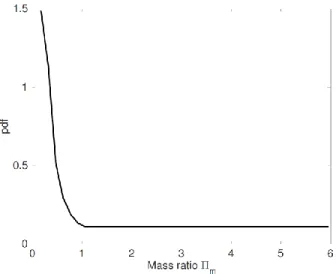
1 values are representative of structures fundamental frequency from 0.5 Hz which is common in the case of isolated or high rise structures to 5 Hz for low rise or rigid structures. For each value of 1, uniform distributions between [0.5 Hz, 5 Hz] are considered for e and2. Here k = 6 and the values (in Hz) of oscillator 1 frequency are: 0.5, 1, 2, 3, 4, 5.As for the mass ratio, values of m2/ m1varying between 1/6 and 6 are considered. To ensure that the mass ratio of the adjacent structures takes reciprocal values with the same probability (e.g. same probability that oscillator 2 is three times heavier or three times lighter than oscillator 1), we do not consider a uniform distribution in [1/6, 6]. Instead, we consider a uniform distribution of m2 / m1 in [1, 6] and also, a uniform distribution of m1/ m2 in [1, 6] (i.e. for 1/6 < m2/ m1< 1). This probability density function is shown Figure 4. Regarding the coefficient
of restitution , a uniform distribution between zero (that corresponds to plastic impact) and one (for elastic impact) is considered. Finally, since the problem is symmetric regarding the mass distribution, and since both 1 and 2 span the same frequency range, we made the choice to
compute sensitivity indexes of the output quantities for oscillator 1 only.
For each value of 1, following Saltelli’s method for the computation of Sobol’’s indexes [41], first, two sample matrices of dimension n×d are considered where d=4 is the number of varying input variables. These samples are generated using the Latin Hypercube Sampling method (LHS) [42]. Then, a total of (d+2)×n runs of the model are required to compute both first order and total sensitivity indexes of all variables. To keep a reasonable computational cost while obtaining accurate estimates of the sensitivity indexes, n = 1000 is considered in this work. In addition, as exposed earlier, the output dimensionless variables are mean values when several signals with the
same excitation amplitude A and filter frequency e are considered. Therefore, five different signals are generated for each sample of input data and the mean output is computed. Of course, only five signals is rather a small sample. Nevertheless, it allows us, to a certain extent, to take into account the variability of excitation signals, even corresponding to the same A and e values, without increasing too much the computational cost. Eventually, there are
30000 5 1000 ) 2 4
( runs for each value of1.
Figure 4. Probability density function of the mass distribution.
Of course, the results of the sensitivity analysis presented in the following sections account only for the sensitivity to the four varying input variables defined in Equations (6). The sensitivity to the structural damping ratio, hardening ratio and dimensionless gap are not studied in this study since they have been assigned constant values. The same holds also for the dimensionless linear limit displacement which is not an independent variable because a constant nonlinear displacement demand was considered.
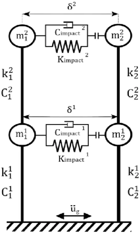
The above sensitivity analysis is quite general since it can investigate the sensitivity of any input-output model. Hence, its application to multi degree of freedom impacting structures is straightforward. Nevertheless, the number of variables increases drastically. For instance, let us consider the two impacting linear elastic 2DOF structures in Figure 5.
Figure 5. Two impacting linear elastic 2DOF structures. In this figure i j m , i j k and i j
C stand for the mass, stiffness and damping coefficient of storey i of structure j respectively and iis the distance between the two structures at storey i. Kimpacti,
i impact
C are the stiffness and damping coefficient of the impact element at storey i. Cimpacti is determined by Kimpacti and the coefficient of restitution i (Equation 1). The counterpart of
Equation (5) reads ) , , , , , , , , , , , , 2 , 2 , 2 , 2 , , , ( 1 1 1 1 1 1 1 1 2 1 1 1 1 1 2 1 1 1 2 1 1 1 1 1 2 2 1 1 1 2 1 1 2 1 2 2 2 2 2 2 1 2 1 2 1 2 2 1 2 1 2 1 1 1 1 1 1 1 1 1 2 2 1 1 1 2 1 1 2 1 max max T k m m A k m A k k K k K m m m m m m k m C k m C k m C k m C k k k k k k u U e e e impact impact i j i j (19)
where max/ imax j i
j u
U
is the dimensionless mean inter-storey drift of storey i of oscillator j . Though the impacting structures in Figure 5 are a very small extension only of the two impacting SDOF oscillators, there is a considerable increase of the number of input parameters (19 instead of 10). Even if some of them are fixed, the number of the varying parameters will remain substantial and thus the computational effort will be considerable. In addition, the number of statistically depended variables increases also.
5. MAXIMUM FORCE AND NONLINEAR DISPLACEMENT DEMAND AMPLIFICATION DUE TO POUNDING
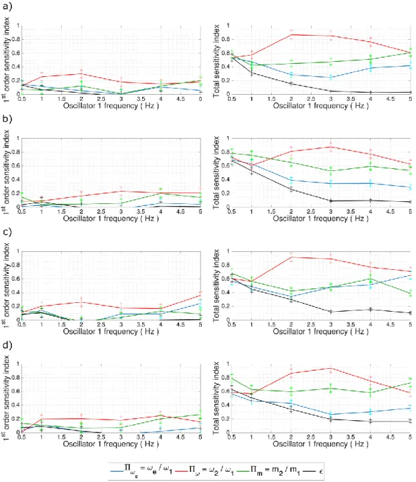
As already mentioned, a sensitivity analysis is performed for each value of oscillator 1 frequency. Hence, in Figure 6, the sensitivity indexes for the maximum force and nonlinear displacement demand amplifications are displayed as functions of oscillator 1 frequency. In addition, the bounds of the 95% confidence intervals are depicted by cross markers. It may be observed that these bounds are quite narrow and thus it is concluded that the accuracy of the results is quite satisfactory.
As a general observation, significant difference is noticed between first order sensitivity indexes and total sensitivity indexes of all input variables. Interactions between variables have an important contribution to the output variability. In general, with a few exceptions, the frequency ratio of the two oscillators is the variable with the highest total sensitivity index for all constitutive laws, the mass ratio coming in second position. In the case oscillator 1 has a low frequency (in particular when f1= 0.5 Hz) all input variables have comparable total sensitivity indexes. In other words, the influences of all variables on the variability of the response of low frequency structures are almost the same.
It is also observed that, the restitution coefficient is the less influential parameter in all cases. Furthermore its influence diminishes with increasing frequency of oscillator 1 up to 3 Hz.
6. INFLUENCE OF POUNDING ON FLOOR RESPONSE SPECTRA
In the case of industrial facilities, the response of sensitive equipment is of paramount importance for the safe and proper function of such facilities during and after an earthquake. The input excitation for equipment and components is determined by the floor response spectra. Therefore, in the case of pounding, its influence on floor response spectra should be investigated.
Figure 6. Sensitivity indexes and their 95 % confidence intervals a) for the dimensionless force amplification of linear elastic oscillators and for the nonlinear demand amplification in the case of b) elastoplastic oscillators, c)
nonlinear elastic oscillators, d) origin oriented oscillators
6.1. Characteristics of floor response spectra of impacting structures
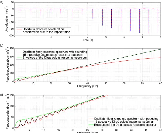
A typical absolute acceleration time history of one of the two impacting oscillators and the corresponding floor response spectrum are shown Figure 7. The two curves in Figure 7a correspond to the time history of the absolute acceleration of the oscillator and the acceleration due to the impact force only (i.e. without the absolute acceleration due to the response to the earthquake excitation). It may be noticed that a) the two curves are quite close, that is, the acceleration of the oscillator is mainly due to the impact force and b) the impact force time
history consists of successive impulses. The duration of these impulses depends on the impact stiffness; the higher the impact stiffness the narrower the impulses. Figure 7b shows that the response spectra corresponding to the above two acceleration time histories are quite close. Consequently, it may be concluded that, in the case of severe pounding, the floor response spectra is governed by the impact impulses. In the same figure, the straight line is the response spectrum of a Dirac pulse whose intensity is equal to the maximum impact impulse. It may be observed that this straight line is close to the initial base slope of the floor response spectrum. Furthermore, for the sake of comparison, the floor response spectrum for the case without pounding is also shown. It may be seen that as expected, impacts influences considerably the overall shape of the floor response spectrum and it results in much higher spectral values, except in the very low frequency range. Since floor response spectra of colliding structures are governed by impact impulses they are much less sensitive to model assumptions (numerical method for impact treatment, time step, size of finite elements in the case of FE models, gap element stiffness etc.) than peak floor accelerations, except at the high frequency range (i.e. periods smaller than the impact duration), with limited practical interest.
To have a further insight into the characteristics of the floor response spectra of pounding structures, let us consider the simplest possible case, an oscillator colliding with a rigid wall subjected to a white noise excitation. The oscillator’s circular frequency and critical damping ratio and the impact stiffness are:0 21rad /s, 0 and Kimpact 100002M
respectively, where M is the oscillator’s mass. Elastic impact is assumed and a zero gap is considered but, of course, similar results are obtained in the case of non-null but small dimensionless gap values as explained in section 3.
As it may be seen in Figure 8, though the impact forces are not strictly speaking periodic, they exhibit some kind of repeatability. Actually we observe that in general (though not always), the time interval between successive impact pulses is equal to T/2, where T 2/0 is the period of the pounding oscillator.
Figure 7. Acceleration response of one of the two impacting oscillators a) Acceleration time history b) Response spectrum.
Based on the above observation we consider an idealized floor acceleration time history composed of N successive identical Dirac pulses repeated every T/2. Because of the periodicity of the considered acceleration, the floor response spectrum will present peaks (i.e. a saw-tooth pattern) at frequencies which are multiple of the fundamental frequency 20. Under these assumptions, an oscillator with circular frequency 2n0 will have exhibited n cycles between two successive pulses. If the relative velocity after the first Dirac is v1, the velocity just before the second pulse will be v2 v1e2n0/0 v1e2n where is the critical damping ratio. The
velocity just after the second pulse will be v2 v1(1e2n) and the velocity after the Nth pulse will be given by the following geometrical progression:
1 1 ) ... 1 ( 2 2 1 ) 1 ( 2 2 2 2 1 n N n N n n n N e e v e e e v v (20)
If 1the maximum displacement is obtained at the end of the first quarter of period after the 𝑁th pulse and thus the pseudoacceleration is:
1 1 2 ) 2 ( 2 2 2 / 0 1 0 nnN e e e n v n PSA (21)
For a large number of pulses 𝑁, the above relation reads:
n e e n v n PSA 0 1 0 /2 2 1 1 2 ) 2 ( (22)
while for high frequencies (i.e. 𝑛 ≫ 1) the pseudoacceleration is that corresponding to only one pulse: 2 / 0 1 0) 2 2 ( n v n e PSA (23)
Figure 8b and 8c depict the numerically computed response spectra corresponding to the acceleration of the impacting oscillator and to an idealized acceleration composed of fifteen successive Dirac pulses. The intensity of the pulses is equal to the maximum impact impulse in Figure 8a. It may be observed that the response spectrum of the periodically repeated Dirac pulses presents all the essential characteristic of the actual floor response spectrum (i.e. shape and saw-tooth pattern in the lower frequencies range). Equation (21), represented by the green line, predicts, also very well, the peak values of this response spectrum. Nevertheless, it may be observed that for high frequencies the 15-Dirac spectrum deviates from the straight line given by equation (23). This is because, for the numerical simulation, the above pulses are not exact theoretical Dirac pulses but triangular pulses with duration 2t, where t0.001s is the time step used for the numerical simulation. Hence, when the response spectrum is computed, due to their finite duration these pulses are not seen as Dirac pulses by high frequency oscillators and their action on these oscillators is not an initial velocity jump. Of course, the above phenomenon
is more pronounced if the duration of the pulses is longer as it happens when impact flexibility is considered. This is confirmed by the response spectrum corresponding to the actual acceleration of the impacting oscillator (red curve) where a finite impact stiffness is considered. Actually this response spectrum (red curve in Figures 8b, 8c)
Figure 8. Acceleration response of an oscillator impacting on a rigid barrier. a) Acceleration time history. b) Response spectra. c) Zoom in on the low frequency range of b).
deviates from the asymptotic straight line sooner than the response spectrum of the idealized acceleration (black curve in Figures 8b,c).
Remark: Though the above, periodic-like impact impulse time history is quite general and occurs in cases like those studied above it should be recognized that different responses are also possible especially for other excitation types. For instance, as already mentioned in the introduction, in the case of harmonic excitation, subharmonic response may arise [25, 27].
For the purpose of the sensitivity study, our desire is to characterize the influence of pounding on floor response spectra with only one output parameter. From the above discussion it is concluded that the maximum impact impulse is such a relevant index. Its sensitivity to the input parameters is presented in the following subsection.
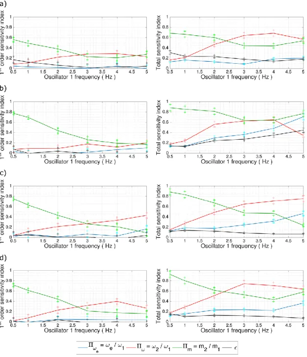
Sensitivity indexes for the dimensionless maximum impact impulse are shown in Figure 9. It is observed that the mass and frequency ratios are, in general, the most influential parameters. In all cases, when the frequency of the oscillator of interest (oscillator 1 in the present case) is less than 2 Hz the influence of the mass ratio is predominant. It is, also, observed that in the case of
Figure 9. Sensitivity indexes and their 95 % confidence intervals for the dimensionless maximum impact impulse. a) linear elastic oscillators, b) elastoplastic oscillators, c) nonlinear elastic oscillators, d) origin oriented oscillators. elastoplastic oscillators the influence of the dimensionless excitation frequency ratio becomes considerable with increasing frequency of the oscillator of interest. The above trends hold for both first order and total sensitivity indexes.
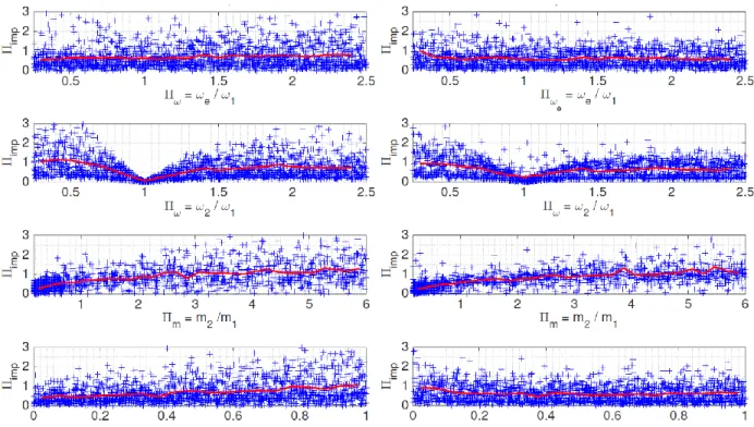
A look at the total and first order sensitivity indexes shows that their differences are smaller than that in the previous section. This implies that the interaction effects are less considerable and that the first order indexes give, by themselves, meaningful information. Hence, it is interesting to study the scatterplots where all data are projected on the plane of the output variable and one input variable. Such examples of scatterplots are represented in Figure 9, for oscillator 1 frequency equal to 2 Hz and for two different constitutive laws (linear elastic and elastoplastic). The red curves correspond to the conditional mean values (i.e. to the mean output value for a given value of the abscissa variable while the remaining variables may take any possible value). Actually, it is reminded that the variances of these conditional mean output variables are the first order sensitivity indexes (equation (17)). In agreement with the sensitivity indexes shown in Figure 9 it is observed that the mean maximum impact impulse exhibits higher variability when it is conditioned on m2/ m1 and on 2/1 especially in the vicinity of
2/
1 1. Of course, themaximum impact impulse is zero for
2/
11(the mean values on the plots are mean values ofclusters, corresponding to small increments on the dimensionless frequency, that is why they are not exactly zero at
2/
11). The mean maximum impact impulse remains small in the vicinity of
2/
11 but it exhibits considerable growth rate while scattering increases, especially in the case of nonlinear constitutive law of the oscillators.Though the coefficient of restitution seems not to be one of the predominant parameters, it is interesting to observe its influence for different constitutive laws (last row of figures in Figure 10). As expected, in the case of elastic impacting structures, the mean maximum impact impulse increases with increasing ε (i.e. less impact dissipation). On the contrary, in the case of elastoplastic oscillators (and nonlinear oscillators, in general, though not shown in Figure 10) the mean maximum impact impulse is much less sensitive to the value of ε.
Figure 10. Scatterplots of the dimensionless maximum impact impulse for an oscillator with a frequency of 2 Hz in the cases of linear elastic (left column) and elastoplastic (right column) constitutive laws. Red lines denotes
conditional mean.
7. CONCLUSIONS
The objective of this work is to gain further insight into the sensitivity of the response of pounding buildings and determine the most influential structural and earthquake excitation parameters. A comprehensive sensitivity analysis was carried out by means of Monte Carlo simulations of two single degree of freedom impacting oscillators. This analysis was performed with Sobol’’s method to compute sensitivity indexes which provide a consistent measure of the relative importance of parameters such as the dimensionless main excitation frequency, the mass and frequency ratios of the structures and the coefficient of restitution. Moreover, the influence of nonlinear behavior of the impacting structures is also considered. The consequences of pounding on the structures themselves, are analyzed in terms of maximum force and nonlinear demand amplification compared to the case without pounding. Contrary to most of the previous studies in this field, this work deals, also, with the influence of pounding on floor response spectra which is of paramount importance for industrial facilities. To this end, the quantity of interest is the maximum impact impulse.
The overall conclusions of this analysis are that the frequency ratio is, in general, the most important parameter as far as maximum force and ductility demand are concerned. Regarding the maximum impact impulse, the mass and frequency ratios are, in general, the most influential parameters, the mass ratio being predominant, for all constitutive laws, in the case of rather low frequencies (e.g. less than 2 Hz) of the oscillator of interest.
Because of the simple model considered here, this work does not cover all aspects of the sensitivity of pounding structures. Increasing the complexity of the models will increase
enormously the number of variables and hence the cost of the sensitivity analysis. Nevertheless we think that the multi-degree of freedom nature of the impacting structures may have a considerable influence of the response leading to results which may differ, to some extent, from those based on SDOF models. Therefore, a future direction could be the extension of this work to the case of impacting 2DOF structures.
ACKNOWLEDGMENT
This work has been partially funded by the French “Agence Nationale de Recherche” through SINAPS@ project.
REFERENCES
1. Shakya K., Pant D.R., Maharjan M., Wijeyewickrema A.C., Maskey P. Lessons learned from performance of buildings during the September 18, 2011 earthquake in Nepal. Asian Journal of Civil
Engineering (BHRC) 2013; 14: 719–733.
2. Anagnostopoulos S. A. Building pounding re-examined: How serious a problem is it? Proceedings of
the 11th World Conference on Earthquake Engineering, Acapulco, Mexico, June 23-28, 1996.
3. Cole G. L., Dhakal R. P., Turner F. M. Building pounding damage observed in the 2011 Christchurch earthquake. Earthquake Engineering and Structural Dynamics 2012; 41:893–913.
4. Gulkan P., Akkar S. Two recent strong motion records from Turkey: Re-interpretation of Bolu (1999) and Bingöl (2003) seismograms. Proceedings of the 3rd UJNR Workshop on Soil-Structure
Interaction, Menlo Park, California, USA, March 29-30, 2004.
5. Bertero V. V., Bresler B., Selna L.G., Chopra A. K., Koretsky A. V. Design implications of damage observed in the Olive View Medical Center buildings. Proceedings of the 5th World Conference on
Earthquake Engineering, Rome, Italy, June 25-29, 1973.
6. Malhotra P. K., Dynamics of seismic pounding at expansion joints of concrete bridges. Journal of
Engineering Mechanics (ASCE) 1998; 124:794–802.
7. Nagarajaiah S., Sun X. Base-isolated FCC building: Impact response in Northridge earthquake.
Journal of Structural Engineering (ASCE) 2001; 129:1063–1075.
8. Rojas F. R., Anderson J. Pounding of an 18-story building during recorded earthquakes. Journal of
Structural Engineering (ASCE) 2012; 138:1530–1544.
9. Papadrakakis M., Mouzakis H. Earthquake simulator testing of pounding between adjacent buildings.
Earthquake Engineering and Structural Dynamics 1995; 24:811–834.
10. Filiatrault A., Wagner P., Cherry S. Analytical prediction of experimental building pounding.
Earthquake Engineering and Structural Dynamics 1995; 24:1131–1154.
11. Jankowski R. Experimental study on earthquake-induced pounding between structural elements made of different building materials. Earthquake Engineering and Structural Dynamics 2010; 39:343–354. 12. Salem Y. S., Feng M. Shake testing of structures retrofitted with viscous dampers to mitigate seismic
pounding. Proceedings of the 13th World Conference on Earthquake Engineering, Beijing, China,
October 12-17, 2008.
13. Papadrakakis M., Mouzakis H., Plevris N., Bitzarakis S. A Lagrange multiplier solution method for pounding of buildings during earthquakes. Earthquake Engineering and Structural Dynamics 1991; 20:981–998.
14. Jankowski R. Non-linear viscoelastic modelling of earthquake-induced structural pounding.
15. Muthukumar S., Desroches R. A Hertz contact model with non-linear damping for pounding simulation. Earthquake Engineering and Structural Dynamics 2006; 35:811–828.
16. Hunt K. H., Crossley F. R. E. Coefficient of restitution interpreted as damping in vibroimpact.
Journal of Applied Mechanics 1975; 42:440–445.
17. Anagnostopoulos S. A. Pounding of buildings in series during earthquakes. Earthquake Engineering
and Structural Dynamics 1988; 16:443–456.
18. Khatiwada S., Chouw N., Butterworth J. W. Evaluation of numerical pounding models with experimental validation. Bulletin of The New Zealand Society for Earthquake Engineering 2013; 46:117–130.
19. Cole G., Dhakal R., Carr A., Bull D. An investigation of the effect of mass distribution on pounding structures. Earthquake Engineering and Structural Dynamics 2011; 40:641–659.
20. Efraimiadou S., Hatzigeorgiou G. D., Beskos D. E. Structural pounding between adjacent buildings subjected to strong ground motions. Part I: The effect of different structure arrangement. Earthquake
Engineering and Structural Dynamics 2013; 42:1509–1528.
21. Efraimiadou S., Hatzigeorgiou G. D., Beskos D. E. Structural pounding between adjacent buildings subjected to strong ground motions. Part II: The effect of multiple earthquakes. Earthquake
Engineering and Structural Dynamics 2013; 42:1529–1545.
22. Madani B., Behnamfar F., Tajmir Riahi H. Dynamic response of structures subjected to pounding and structure-soil-structure interaction. Soil Dynamics and Earthquake Engineering 2015; 78:46-60. 23. Mahmoud S., Abd-Elhamed A., Jankowski R. Earthquake-induced pounding between equal height
multi-storey buildings considering soil-structure interaction. Bulletin Earthquake Engineering 2013; 11:1021-1048.
24. Ghandil M., Aldaikh H. Damage-based planar pounding analysis of adjacent symmetric buildings considering inelastic structure-soil-structure interaction. Earthquake Engineering and Structural
Dynamics 2017; 46:1141–1159.
25. Davis R. Pounding of buildings modelled by an impact oscillator. Earthquake Engineering and
Structural Dynamics 1992; 21:253–274.
26. Chau K. T., Wei X. X. Pounding of structures modelled as non-linear impact of two oscillators.
Earthquake Engineering and Structural Dynamics 2001; 30:633–651.
27. Thompson J. M. T, Stewart H. B. Nonlinear Dynamics and Chaos. Wiley& Sons, Ltd. 1986.
28. Dimitrakopoulos E., Kappos A., Makris N. Dimensional analysis of yielding and pounding structures for records with distinct pulses. Soil Dynamics and Earthquake Engineering 2009; 29:1170–1180. 29. Dimitrakopoulos E., Makris N., Kappos A. Dimensional analysis of the earthquake-induced pounding
between adjacent structures. Earthquake Engineering and Structural Dynamics 2009; 38:867–886. 30. Dimitrakopoulos E., Makris N., Kappos A. Dimensional analysis of the earthquake-induced pounding
between inelastic structures. Bulletin Earthquake Engineering 2011; 9:561–579.
31. Caniou Y. Analyse de sensibilité globale pour les modèles imbriqués et multiéchelles. PhD Thesis,
Institut Français de Mécanique Avancée 2012.
32. Sobol’ I.M. Sensitivity estimates for non-linear mathematical models. Mathematical Modeling and
Computational Experiment 1993; 1:407–414.
33. Barenblatt GI. Scaling, Self-Similarity, and Intermediate Asymptotics. University Cambridge, 1996. 34. Anagnostopoulos S.A. Equivalent viscous damping for modeling inelastic impacts in earthquake
pounding problems. Earthquake Engineering and Structural Dynamics 1992; 33:897–902.
35. Kanai K. Semi-empirical formula for the seismic characteristics of the ground. Bulletin of Earthquake
Research institute of Tokyo 1957; 35:309–325.
36. Clough R.W., Joseph P. Dynamic of Structures, first ed. McGraw-Hill Intl. Ed. 1975.
37. Priestley M.J.N., Macrae G.A. Seismic test of precast beam-to-column joint subassemblages with unbonded tendons. PCI Journal 1996; 41:64–81.
38. Building Seimic Safety Council. NEHRP recommended provisions for seismic regulations for new
39. CEN, European Committee for Standardization. Eurocode 8: Design Provision for Earthquake
Resistance of Structures. EN 1998-1: 2004. Comitée Européen de Normalisation, Brussels, 2004.
40. Hoeffding W. A class of statistics with asymptotically normal distribution. The Annals of
Mathematical Statistics 1948; 19:293–325.
41. Saltelli A, Ratto M, Andres T, Campolongo F, Cariboni J, Gatelli D, Saisana M, Tarantola S. Global
Sensitivity Analysis. John Wiley & sons Ltd. 2008.
42. Saltelli A., Annoni P., Azzini I., Campolongo F., Ratto M., Tarantola S. Variance based sensitivity analysis of model output. Design and estimator for the total sensitivity index. Computer Physics