HAL Id: hal-00733471
https://hal-upec-upem.archives-ouvertes.fr/hal-00733471
Submitted on 19 Sep 2012
HAL is a multi-disciplinary open access
archive for the deposit and dissemination of
sci-entific research documents, whether they are
pub-lished or not. The documents may come from
teaching and research institutions in France or
abroad, or from public or private research centers.
L’archive ouverte pluridisciplinaire HAL, est
destinée au dépôt et à la diffusion de documents
scientifiques de niveau recherche, publiés ou non,
émanant des établissements d’enseignement et de
recherche français ou étrangers, des laboratoires
publics ou privés.
Image reconstruction from multiple sensors using Stein’s
principle. Application to parallel MRI
Alexandru Marin, Caroline Chaux, Jean-Christophe Pesquet, Philippe Ciuciu
To cite this version:
Alexandru Marin, Caroline Chaux, Jean-Christophe Pesquet, Philippe Ciuciu. Image reconstruction
from multiple sensors using Stein’s principle. Application to parallel MRI. ISBI 2011, Mar 2011,
United States. �hal-00733471�
IMAGE RECONSTRUCTION FROM MULTIPLE SENSORS USING STEIN’S PRINCIPLE.
APPLICATION TO PARALLEL MRI.
Alexandru Marin
1, Caroline Chaux
1, Jean-Christophe Pesquet
1and Philippe Ciuciu
21
Univ. Paris-Est, LIGM UMR CNRS 8049
5 Bd Descartes, 77454 Marne-la-Vall´ee, France
E-mails:[email protected],{caroline.chaux,jean-christophe.pesquet}@univ-paris-est.fr
2
CEA/DSV/I2BM/Neurospin, CEA Saclay,
Bat. 145, Point Courrier 156, 91191 Gif-sur-Yvette cedex, France.
E-mail:[email protected]
ABSTRACT
We are interested in image reconstruction when data provided by several sensors are corrupted with a linear operator and an additive white Gaussian noise. This problem is addressed by invoking Stein’s Unbiased Risk Estimate (SURE) techniques. The key advantage of SURE methods is that they do not require prior knowledge about the statistics of the unknown image, while yielding an expression of the Mean Square Error (MSE) only depending on the statistics of the ob-served data. Hence, they avoid the difficult problem of hyperparam-eter estimation related to some prior distribution, which traditionally needs to be addressed in variational or Bayesian approaches. Con-sequently, a SURE approach can be applied by directly parameter-izing a wavelet-based estimator and finding the optimal parameters that minimize the MSE estimate in reconstruction problems. Simu-lations carried out on parallel Magnetic Resonance Imaging (pMRI) images show the improved performance of our method with respect to classical alternatives.
Index Terms— Reconstruction, Stein’s principle, wavelets,
nonlinear estimation, multiple sensors, pMRI.
1. INTRODUCTION
Much attention has been paid to Stein’s principle [1] in the recent statistical literature in order to derive MSE estimates in statistical problems involving an additive Gaussian noise. In particular, it was successfully used in wavelet-based nonlinear denoising [2]. More re-cently, such an approach was extended to deconvolution problems [3, 4] and it was also employed for Poisson data denoising [5]. The key advantage of Stein’s principle [6] is that it does not require prior knowledge about the statistics of the unknown image. Hence, it al-lows us to circumvent the difficult problem of the estimation of the hyperparameters of a prior distribution as frequently encountered in Bayesian approaches.
In this paper, we propose to further extend the scope of Stein-based approaches by addressing image reconstruction problems. More precisely, we employ Stein’s principle in order to propose a wavelet-based estimator relying on Linear Expansion of Thresh-olds (LET) functions [7, 8]. This enables us to design efficient medi-cal image reconstruction algorithms whose parameters are optimally computed to achieve the minimum MSE. The estimator operates in
THIS IS AN INVITED PAPER IN THE SPECIAL SESSION ON “WAVELETS AND NEUROIMAGING”.
the wavelet transform domain and deals with mutiple observations delivered by several sensors. The interest of this method is demon-strated in the parallel Magnetic Resonance Imaging (pMRI) context [9, 10]. Recall that this modality offers a means of significantly reducing the acquisition time at the expense of a degraded signal-to-noise ratio. In a recent work by Chaˆari et al. [11] a novel method based on a wavelet-based variational approach was proposed, which makes use of an iterative optimization algorithm to compute the Maximum A Posteriori (MAP) estimate. We aim here at proposing a faster non-iterative method where the estimator parameters are adjusted automatically. Note also that the proposed approach is very flexible concerning the wavelet choice and the estimator form.
The remainder of the paper is organized as follows. In Section 2, we briefly introduce the notation and describe the considered in-verse problem. Then, Section 3 is devoted to the proposed statistical method. In particular, we show how to address the complex-valued nature of the data and build an unbiased quadratic risk estimator, be-fore discussing the estimator choice. Finally, in Section 4, we illus-trate the effectiveness of our reconstruction algorithm on a simulated set of pMRI data.
2. PROBLEM STATEMENT 2.1. Notations
We consider here pMRI images generated by consideringL
acquisi-tion coils and a reducacquisi-tion factorR. Let X× Y be the dimensions
of the full Field Of View (FOV) image, along the respective phase and and frequency directions. The reduced FOV image size in phase encoding direction is thus given by∆X =X
R. B will denote the set
of spatial indices in the reduced FOV image.
2.2. Observation model
At each position x ∈ B we observe an L-dimensional data vector d(x) = [d1(x), . . . , dL(x)]⊤, which is obtained by applying an
L× R sensitivity matrix S(x) given by
S(x) = 2 6 4 S1(x1, x2) . . . S1(x1, x2+ (R − 1)∆X) .. . · · · ... SL(x1, x2) . . . SL(x1, x2+ (R − 1)∆X) 3 7 5 ,
to anR-dimensional vector of pixel values in the original (unknown)
1)∆X)]⊤
and by adding a complex Gaussian circular noise vector corrupting samples from all coils: n(x) = [n1(x), . . . , nL(x)]⊤.
Here ρ(x) is an R-dimensional random field which is assumed to be
independent of n(x). The between-coil noise covariance matrix is
given by Cov{n(x), n(x′)} = Ψδ(x − x′), ∀(x, x′) ∈ B2. The
resulting model is consequently described by the following linear model:
d(x) = S(x)ρ(x) + n(x), ∀x ∈ B. (1) The objective of this work is to recover ρ from d knowing S.
3. PROPOSED METHOD 3.1. Complex nature of the data
In MRI, the acquired data are complex-valued even if the magnitude is only considered for visualization purpose. Let·R and·Ibe the
subscripts indicating the real and imaginary parts (namely,ℜ{·} and ℑ{·}) of the data. The observed data can thus be expressed by
» dR(x) dI(x) – = » SR(x) −SI(x) SI(x) SR(x) – » ρR(x) ρI(x) – + » nR(x) nI(x) –
so that Model (1) can be reexpressed under the form
dC(x) = SC(x)ρC(x) + nC(x), ∀x ∈ B, (2)
where the involved vectors and matrices are real-valued. Assuming that we are able to compute the pseudo-inverse S†C(x) of SC(x)
defined by
S†C(x) =“SC(x)⊤SC(x)
”−1
SC(x)⊤, (3)
it follows thatρeC(x) = ρC(x) +neC(x) where
e
ρC(x) = S†C(x)dC(x) and neC(x) = S†C(x)nC(x).
Furthermore, the following relations regarding the second-order statistics of the random fieldneC(x) will be useful for the quadratic
risk computation: Cov{neC(x),neC(x)} = S†C(x)ΨC ` S†C(x)´⊤ (4) Cov{neC(x), nC(x)} = S†C(x)ΨC. (5) where Cov{nC(x), nC(x′)} = ΨCδ(x − x′), ∀(x, x′) ∈ B2. 3.2. Derivation of the SURELET estimator
For every x ∈ B and k ∈ {1, . . . , K}, let ϕk(x) ∈ R2L be an
analysis vector and letϕek(x) ∈ R2Rbe a synthesis vector. In the
case of a decomposition onto a basis of the FOV image,K= XY
and the need of2K functions stems from the fact that the real and
imaginary parts of the data are considered. We choose an estimator of the form
∀k ∈ {1, . . . , 2K}, ρbk= θk(wk) (6)
wherewk =
P
x∈Bϕk(x)⊤dC(x) and θk: R → R is some
dif-ferentiable estimating function (the choice of this function will be discussed in Section 3.4). Then the estimator of ρC(x) is given by
b ρC(x) = 2K X k=1 b ρkϕek(x) (7)
The objective now is to compute the estimator parameters that mini-mize the quadratic risk.
3.3. Unbiased risk estimate
The risk corresponding to a MSE estimation is defined as:∀x ∈ B,
E˘kρbC(x) − ρC(x)k2 ¯ = E˘kρbC(x) −ρeC(x) +enC(x)k2 ¯ = E˘kρbC(x) −ρeC(x)k2 ¯ + 2EnρbC(x)⊤enC(x) o − 2EnρeC(x)⊤enC(x) o + E˘kenC(x)k2¯. (8) Here, we focus on the second term which, by using (7), reads:
EnρbC(x)⊤neC(x) o = 2K X k=1 e ϕk(x)⊤E{bρkenC(x)}.
In addition, applying the analysis vectors ϕk(x) to dC(x) yields
coefficientswkwhich can be decomposed aswk= uk+ nk, where
uk= X x∈B ϕk(x)⊤SC(x)ρC(x) nk= X x∈B ϕk(x)⊤nC(x),
so thatρbkcan be rewritten as
b
ρk= θk(wk) = θk(uk+ nk). (9)
Then, by applying Stein’s principle [1], it follows that: E{bρkneC(x)} = E
˘ θ′k(wk)
¯
E{nkenC(x)}. (10)
After some tedious calculations, it follows that the quadratic risk estimate reads: E˘kρbC(x) − ρC(x)k2 ¯ = E˘kρbC(x) −ρeC(x)k2 ¯ + 2 2K X k=1 E˘θ′k(wk) ¯ e ϕk(x)⊤S†C(x)ΨCϕk(x) − tr“S†C(x)ΨC ` S†C(x)´⊤”.
An unbiased estimate of the resulting global MSE is:
b E(bρC− ρC) = bE(bρC−ρeC) + ∆ (11) where b E(ρbC−ρeC) = 1 XY X x∈B kρbC(x) −ρeC(x)k2 and ∆ = 2 XY 2K X k=1 θk′(wk) X x∈B e ϕk(x)⊤S†C(x)ΨCϕk(x) − 1 XY X x∈B tr “ S†C(x)ΨC ` S†C(x)´⊤”.
Note that the risk estimate is expressed in terms of observed data only. Now, the next step consists of specifying the form of the es-timating functionsθkin order to find the parameters that minimize
3.4. Estimating function choice
Assume that the coefficients(wk)1≤k≤2K are classified according
toM ∈ N∗
distinct nonempty index subsets (e.g. wavelet subbands)
Km,m∈ {1, . . . , M }. For every m ∈ {1, . . . , M } and k ∈ Km,
we choose subband-dependent estimating functions of the form:
θk(wk) = Im
X
i=1
am,ifm,i(wk) (12)
where(am,i)1≤i≤Im are scalar real-valued weighting factors and,
for everyi∈ {1, . . . , Im}, fm,i: R → R is a differentiable
func-tion. These functions are the Linear Expension of Thresholds (LET) estimating functions introduced in [7, 8] and correspond to a linear combination ofIm∈ N∗given univariate functionsfm,iapplied to
wk(note that we use the same estimating function for a given Km). 3.5. Computation of(am,i)1≤i≤Imparameters
As mentioned earlier, we want to compute the parameters(am,i)1≤i≤Im
that minimize the quadratic risk in (11). It can be shown that this amounts to solving the following set of linear equations:
∀m ∈ {1, . . . , M }, ∀i ∈ Im, M X n=1 In X j=1 an,j X x∈B βm,i(x)⊤βn,j(x) =X x∈B βm,i(x)⊤ρeC(x) − X k∈Km fm,i′ (wk) X x∈B e ϕk(x)⊤S†C(x)ΨCϕk(x) whereβm,i(x) =Pk∈K mfm,i(wk)ϕek(x). 4. SIMULATION RESULTS 4.1. Context
In our experiments, the families of analysis/synthesis functions are chosen such that
ϕk(x) = SC(x) “ SC(x)⊤SC(x) + λI ”−1 | {z } G(x) ψk(x) e ϕk(x) = eψk(x)
whereλ >0, I is the identity matrix and the components of vector ψk(x) (resp. eψk(x)) are obtained from shifted versions of a 2D
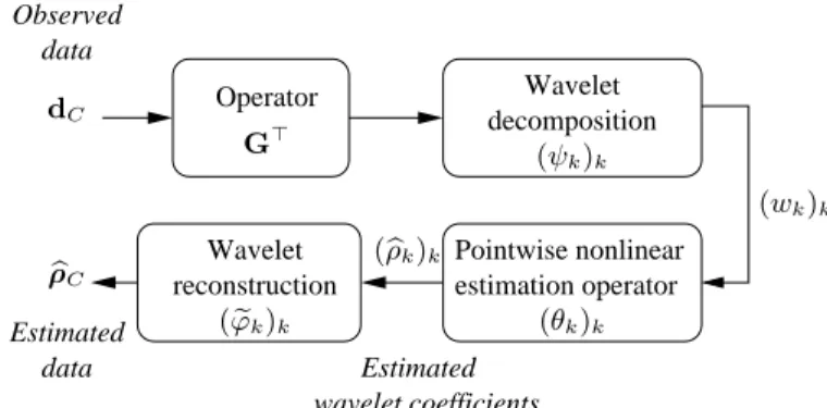
separable wavelet analysis function (resp. synthesis function). A scheme summarizing the proposed reconstruction approach is given in Fig. 1.
Concerning the estimating functions, we chooseIm= 2. fm,1
is the identity function and
∀ρ ∈ R, fm,2(ρ) = „ 1 − exp“− ρ 8 (ωσm)8 ”« ρ
whereω ∈]0, ∞[ and σmis the standard deviation of(nk)k∈Km.
These LET estimating functions were introduced in [7].
We compare our results with SENSE reconstruction [9], which is based on a weighted least-squares estimator:
b ρSENSE(x) = “` S∗(x)´⊤Ψ−1S(x)”†`S∗(x)´⊤Ψ−1d(x). Pointwise nonlinear estimation operator Estimated wavelet coefficients Wavelet decomposition Wavelet reconstruction Observed data Estimated data Operator ( eϕk)k (θk)k dC b ρC (ψk)k (wk)k (bρk)k G⊤
Fig. 1. Flowchart of the proposed reconstruction method.
4.2. Numerical results
To assess the performance of the proposed method, we simulated synthetic data from a full FOV reference image displayed in Fig. 2(a) according to model (1). Note that the dynamic range of the absolute value of the pixels is large.
The number of antennas is here equal toL = 8 and the
reduc-tion factor isR= 4. The covariance matrix of the noise ψ is chosen
to be diagonal (no between coil correlation) and all the diagonal en-tries are chosen equal toσ2(homoscedasticity). Next, we compared our results with those provided by the classical SENSE reconstruc-tion. Here, an orthonormal wavelet analysis (symlets of length 8) is performed on4 resolution levels. The regularization parameter λ
was chosen empirically. Typical values around0.001 were observed
to provide accurate and reliable results. The performance was mea-sured in terms of Peak Signal-to-Noise Ratio (PSNR) as reported in Table 1. In short, our method enables a significant gain in PSNR values with respect to the SENSE approach.
Table 1. PSNR values for reconstructed images (in dB).
Method Real Part Imag. Part Magn.
σ2= 5 106 SENSE 36.29 35.48 38.75 λ= 10−3 38.28 36.77 40.43 Proposed λ= 10−4 38.30 36.79 40.46 λ= 10−5 38.30 36.79 40.46 σ2= 12.5 105 SENSE 42.94 42.40 45.58 Proposed λ= 10−4 43.57 42.74 46.35 σ2= 2 107 SENSE 30.00 28.57 32.03 Proposed λ= 10−4 33.72 31.69 34.92
Interestingly, the larger the noise, the stronger the PSNR im-provements we observed in favour of the proposed approach. For vi-sualization purposes, the reconstructed images by SENSE and Stein-Let methods are shown in Fig. 2(b)-(c) whenσ2 = 5 106. The
main differences can be observed in the center of the images where more residual noise is found for SENSE reconstruction. Note that the Stein-LET reconstruction in Fig. 2(c) is achieved in about 15 s. on a Xeon(R) CPU [email protected].
(a) (b) (c)
(d) (e) (f)
Fig. 2. (a): Magnitude of the reference image: range in [0,91496]. (b)-(c): Magnitude of the restored images by SENSE and the proposed
Stein-LET approach, respectively. (d)-(f): zoomed versions of images (a)-(c) on the central part of the brain to illustrate the noise reduction using the Stein-LET estimator.
5. CONCLUSION
We proposed a new reconstruction method based on Stein’s principle and LET functions which was applied to pMRI. In this context, our approach provides more accurate results than the classical SENSE alternative. In our approach, most of the parameters are set in an unsupervised manner. In addition, the computational complexity is quite reasonable. In the future, we plan to validate this restoration method in a more realistic context i.e. without knowing the amount of noise and using an unperfectly known sensitivity matrix. Fur-thermore, we will consider 3D decomposition to extend the present contribution and enable the reconstruction of all slices simultane-ously. It would be also interesting to apply this approach to other reconstruction strategies [12, 13].
6. REFERENCES
[1] C. Stein, “Estimation of the mean of a multivariate normal distribution,” Ann. Stat., vol. 9, no. 6, pp. 1135–1151, Nov. 1981.
[2] D. L. Donoho and I. M. Johnstone, “Adapting to unknown smoothness via wavelet shrinkage,” J. American Statist. Ass., vol. 90, pp. 1200–1224, Dec. 1995.
[3] J.-C. Pesquet, A. Benazza-Benyahia, and C. Chaux, “A SURE approach for digital signal/image deconvolution problems,”
IEEE Trans. Signal Process., vol. 57, no. 12, pp. 4616–4632,
Dec. 2009.
[4] C. Chesneau, M.J. Fadili, and J.-L. Starck, “Stein block thresh-olding for wavelet-based image deconvolution,” Electronic Journal of Statistics, vol. 4, pp. 415–435, 2010.
[5] F. Luisier, T. Blu, and M. Unser, “Undecimated Haar thresh-olding for Poisson intensity estimation,” in Proc. of the 2010
IEEE Int. Conf. on Image Processing (ICIP’10), Hong Kong,
People’s Republic of China, Sep. 26-29, 2010, pp. 1697–1700. [6] M. Raphan and E. P. Simoncelli, “Learning least squares es-timators without assumed priors or supervision,” Tech. Rep. Computer Science TR2009-923, Courant Inst. of Mathemati-cal Sciences, New York University, Aug. 2009.
[7] T. Blu and F. Luisier, “The SURE-LET approach to image denoising,” IEEE Trans. Image Process., vol. 16, no. 11, pp. 2778–2786, Nov. 2007.
[8] J.-C. Pesquet and D. Leporini, “A new wavelet estimator for image denoising,” in IEE Sixth Int. Conf. Im. Proc. Appl., Dublin, Ireland, Jul. 14-17 1997, vol. 1, pp. 249–253. [9] K. P. Pruessmann, M. Weiger, M. B. Scheidegger, and P.
Boe-siger, “SENSE: sensitivity encoding for fast MRI,” Magnetic
Resonance in Medicine, vol. 42, no. 5, pp. 952–962, Jul. 1999.
[10] C. Rabrait, P. Ciuciu, A. Rib`es, C. Poupon, P. Leroux, V. Lebon, G. Dehaene-Lambertz, D. Le Bihan, and F. Lethi-monnier, “High temporal resolution functional MRI using par-allel echo volume imaging,” Magnetic Resonance Imaging, vol. 27, no. 4, pp. 744–753, Mar. 2008.
[11] L. Chaˆari, J.-C. Pesquet, A. Benazza-Benyahia, and P. Ciu-ciu, “A wavelet-based regularized reconstruction algo-rithm for SENSE parallel MRI with applications to neu-roimaging,” Medical Image Analysis, 2011, In press, doi:10.1016/j.media.2010.08.001.
[12] J. Petr, J. Kybic, M.l Bock, S. M¨uller, and V. Hlav´a˘c, “Parallel image reconstruction using B-spline approximation (PROBER),” Magn. Reson. Med., vol. 58, no. 3, pp. 582–591, Sep. 2007.
[13] A. A. Samsonov, “On optimality of parallel MRI reconstruc-tion in k-space,” Magn. Reson. Med., vol. 59, no. 1, pp. 156– 164, Jan. 2008.
![Fig. 2. (a): Magnitude of the reference image: range in [0,91496]. (b)-(c): Magnitude of the restored images by SENSE and the proposed Stein-LET approach, respectively](https://thumb-eu.123doks.com/thumbv2/123doknet/13000385.379933/5.892.215.705.88.446/magnitude-reference-magnitude-restored-images-proposed-approach-respectively.webp)
