HAL Id: halshs-00586059
https://halshs.archives-ouvertes.fr/halshs-00586059
Preprint submitted on 14 Apr 2011
HAL is a multi-disciplinary open access archive for the deposit and dissemination of sci-entific research documents, whether they are pub-lished or not. The documents may come from teaching and research institutions in France or
L’archive ouverte pluridisciplinaire HAL, est destinée au dépôt et à la diffusion de documents scientifiques de niveau recherche, publiés ou non, émanant des établissements d’enseignement et de recherche français ou étrangers, des laboratoires
Financial development, entrepreneurship and job
satisfaction
Milo Bianchi
To cite this version:
WORKING PAPER N° 2008 - 59
Financial development, entrepreneurship
and job satisfaction
Milo Bianchi
JEL Codes: L26, J20, G20
Keywords: Financial development, entrepreneurship, job
satisfaction
P
ARIS-
JOURDANS
CIENCESE
CONOMIQUESL
ABORATOIRE D’E
CONOMIEA
PPLIQUÉE-
INRA48,BD JOURDAN –E.N.S.–75014PARIS TÉL. :33(0)143136300 – FAX :33(0)143136310
www.pse.ens.fr
CENTRE NATIONAL DE LA RECHERCHE SCIENTIFIQUE – ÉCOLE DES HAUTES ÉTUDES EN SCIENCES SOCIALES ÉCOLE NATIONALE DES PONTS ET CHAUSSÉES – ÉCOLE NORMALE SUPÉRIEURE
Financial Development, Entrepreneurship,
and Job Satisfaction
Milo Bianchiy
Paris School of Economics February 9, 2009
Abstract
This paper shows that utility di¤erences between the self-employed and the employees increase with …nancial development. This e¤ect is not explained by increased pro…ts but by an increased value of non-monetary bene…ts, in particular job independence. We interpret these …ndings by building a simple occupational choice model in which …-nancial constraints may impede …rms’ creation and depress labor de-mand, thereby pushing some individuals into self-employment for lack of salaried jobs. In this setting, …nancial development favors a better matching between individual motivation and occupation, thereby in-creasing entrepreneurial utility despite inin-creasing competition and so reducing pro…ts.
Keywords: Financial development; entrepreneurship; job satisfac-tion.
JEL codes: L26, J20, G20.
Sincere thanks to Abhijit Banerjee, Erik Lindqvist and Jörgen Weibull for very helpful discussions. I have also bene…ted from comments by Cedric Argenton, Andrew Clark, Tore Ellingsen, Fabrice Etilé, Justina Fischer, Thibault Fally, Peter Haan, Andrew Oswald, Thomas Piketty, Asa Rosen, Giancarlo Spagnolo; and from presentations at Stockholm School of Economics, Paris School of Economics, Northwestern University, UNU-Wider, IFN. Financial support from the Knut and Alice Wallenberg Foundation and from Région Ile-de-France is gratefully acknowledged.
1
Introduction
From a standard economic viewpoint, the choice of becoming an entrepre-neur displays some puzzling features. First, it is on average unpro…table: returns to capital are too low and risk too high (Hamilton, 2000; Moskowitz and Vissing-Jorgensen, 2002). Second, it seems to deliver high utility: en-trepreneurs often report higher levels of job satisfaction than employees with similar characteristics (Blanch‡ower and Oswald, 1998; Hundley, 2001; Benz and Frey, 2004). A popular explanation to these puzzles posits that being an entrepreneur gives substantial non-monetary bene…ts and that, due to …nan-cial barriers to entry, entrepreneurs can enjoy utility above market clearing (Blanch‡ower and Oswald, 1998).
In this paper, we examine the above argument by exploring both theo-retically and empirically how utility di¤erences between entrepreneurs and employees respond to …nancial development. In this way, our analysis may contribute to a better understanding of occupational choices, as driven by these utility di¤erences, in relation in particular to market conditions.
More speci…cally, we …rst build an occupational choice model in which individuals can choose between becoming an entrepreneur, which requires investing capital and hiring workers, or look for a job as an employee. The model builds on two main ingredients. First, in addition to pro…ts and wages, individuals value also non-monetary dimensions of their job. For example, entrepreneurs may derive utility from being their own boss.1 In line with the evidence in Fuchs-Schündeln (2008), we assume that individuals may di¤er in how much they like (or dislike) not having a boss, and so more generally in their (intrinsic) motivation for becoming an entrepreneur.
The second key ingredient is that labor demand is bound by the amount of individuals who become entrepreneurs. If entrepreneurs are a few, labor demand is low and so is the probability of …nding a salaried job. This may push some individuals to become entrepreneurs by lack of better opportu-nities.2 In this way, we incorporate the view that individuals may start their businesses with very di¤erent motivations. On the one hand, they may choose to be entrepreneurs, as it is typically the case in more developed countries.3 On the other, they may become entrepreneurs by necessity. A substantial fraction of entrepreneurs in developing countries falls into this category (Reynolds, Bygrave, Autio, Cox and Hay, 2002), and these
indi-1
See for example Taylor (1996), Blanch‡ower and Oswald (1998), Hamilton (2000), Benz and Frey (2004).
2
In most existing occupational choice models, instead, entrepreneurs have chosen to be so and they could have become employees, while employees for some reason could not become entrepreneurs. However, if this were the case, entrepreneurs would always be better o¤ than employees, which seems at odds with the evidence mentioned next and it will not be true in our data.
3
See for example Parker (2004) and Bianchi and Henrekson (2005) for a review of such class of models of entrepreneurship.
viduals may be very happy to leave their businesses for a salaried job.4 We then explore the e¤ects of …nancial development in such setting. While the relation between …nancial constraints and occupational choices has received signi…cant attention (see Banerjee and Du‡o, 2005 and Levine, 2005 for recent surveys), we here focus on the rather unexplored aspect of how …nancial development may a¤ect individual utility, and in particular the non-monetary returns from entrepreneurship. As mentioned above, and as con…rmed also in our analysis, such returns seem a crucial component of entrepreneurial choices.
In our model, …nancial development allows some poor to access credit and set up a …rm, which in turn increases competition and the demand for labor. In this way, the poor and more motivated individuals can become entrepreneurs, while the rich and less motivated individuals are induced to look for a salaried job. It follows that higher levels of …nancial development are associated with more satis…ed entrepreneurs, and this is the case even if …nancial development increases competition and so reduces pro…ts. In fact, in more …nancially developed countries, individuals tend to have chosen to be entrepreneurs because of their particular motivation rather than for lack of a better job.
These predictions are tested by using individual data on job satisfaction taken from the World Value Surveys, which provide comprehensive house-hold surveys for a large set of countries over two decades. We focus on self-reported levels of job satisfaction in order to account both for monetary and non-monetary returns from a job, which is crucial in our framework since pro…ts and utility need not move in the same direction. Furthermore, in addition to standard demographic variables, these data provide informa-tion on beliefs, personality and di¤erent dimensions of individual jobs, which permits to test whether …nancial development works through these channels. Finally, while most of the evidence on entrepreneurs’job satisfaction comes from OECD countries, these data cover a wide sample of developing and developed country. This allows drawing a broader picture of whether entre-preneurship has di¤erent meanings, and …nancial development has di¤erent e¤ects, according to a country’s stage of development.
Our main …ndings lend support to the predictions of the model. First, descriptive statistics show that entrepreneurs report higher levels of job sat-isfaction than employees only in more …nancially developed countries and
4See Banerjee and Du‡o (2008) for a detailed account of this view in developing
coun-tries and Reynolds, Bygrave, Autio, Cox and Hay (2002) for comprehensive surveys on necessity vs. opportunity entrepreneurs. Relatedly, see the literature on formality vs. in-formality (Harris and Todaro, 1970; Loayza, 1994; Schneider and Enste, 2000) and survival vs. growth enterprises (Berner, Gomez and Knorringa, 2008). On developed countries, see the literature on self-employment as a way out unemployment (e.g. Evans and Leighton, 1989; Glocker and Steiner, 2007; Andersson and Wadensjö, 2007), and as a response to labor market discrimination (Borjas, 1986).
that, in these countries, entrepreneurs tend to report lower income than em-ployees. These patterns are con…rmed in a more structured analysis in which we control for a set of individual variables and for country-year …xed e¤ects. It emerges that entrepreneurial utility, relative to the one of employees, in-creases with …nancial development. This result is robust to the inclusion of additional macroeconomic variables, accounting for example for better institutions or economic perspectives, as well as to the use of alternative measures of …nancial development. Moreover, this e¤ect appears stronger in less …nancially developed countries, where many individuals become en-trepreneurs by necessity and so many would be happy to switch to a salaried employment.
Finally, we explore which mechanisms may underlie such relation. We …rst notice that adding income among the explanatory variables does not change our results. Income appears (as expected) a strong determinant of job satisfaction, but higher …nancial development does not increase entre-preneurs’ utility by making them richer. On the other hand, the e¤ect of …nancial development becomes insigni…cant once we control for the degree of independence enjoyed in the job. This suggests that higher …nancial de-velopment allows entrepreneurs to enjoy higher non-monetary bene…ts, and in particular higher freedom in taking decisions in their job.
We present our model and theoretical analysis in Sections 2 and 3, re-spectively; Section 4 describes our data and Section 5 reports the empirical results; Section 6 concludes by discussing some policy implications. Omitted proofs and tables are reported in the Appendix.
2
The Model
Consider an economy populated by a unitary mass of risk-neutral individ-uals. Each individual is characterized by a type (a; b); where a describes his initial wealth and b his taste for being an entrepreneur (which for now we simply call motivation). Wealth is drawn from a smooth cumulative dis-tribution function F with density f ; motivation from a smooth cumulative distribution function G with density g. These draws are assumed to be sta-tistically independent. In addition, each individual is endowed with one unit of labor, which he may employ either for setting up a …rm or to work as an employee. We now describe these options in further detail.
2.1 Options
First, an individual can set up a …rm. We assume that each …rm produces the same homogeneous good and it has the same size: it employs k units of capital, l workers, and it produces q units of output. The pro…t is then
where p denotes the price of the good, w denotes workers’wage, and r is the market interest rate. In addition, managing a …rm gives utility b. Hence, an individual who sets up a …rm enjoys utility
U1 = + b: (2)
These individuals are called entrepreneurs, and we denote their population share with x1. As a second option, an individual can look for a job in one of these …rms. If he is hired, he enjoys utility
U2= w:
The population share of workers is denoted with x2: If he is not hired, he remains idle and enjoys some utility which we normalize to zero.
2.2 Markets
There are three markets in our economy: a labor market, a product market and a credit market. In the labor market, the wage w is bounded below by w, which implies that such market may display excess supply. In such case, each applicant has the same probability of getting a job.5 The number of workers equals …rms’demand, so we have
x2= lx1: (3)
The product market is described by a decreasing inverse demand function
p = P (Q); (4)
where Q = x1q denotes the total output produced in the economy. Entre-preneurs take the price p as given, and inelastically supply their output.
The …nancial market is competitive, the interest rate r is …xed and ex-ogenous, and we normalize it to one. An individual with wealth a can ask for a loan (k a) in order to set up a …rm: However, ex-post moral hazard limits the maximum size of such loan. Since, at cost c; such individual can renege on his loan contract and run away with the money, the required repayment (k a) cannot exceed c. Hence, only individuals with enough wealth can set up a …rm, and we de…ne such lower bound on wealth as
a k c: (5)
The threshold a decreases with c, which measures how easy it is to enforce loan contracts and so it is an indicator of …nancial development.6
5
More sophisticated reasons for non-market clearing wages are for example in Weiss (1980) and Shapiro and Stiglitz (1984).
6
Baner-2.3 Equilibrium
In equilibrium, each individual, given his type, chooses an option in or-der to maximize his expected utility and the markets function according to equations (3), (4) and (5). In such equilibrium, there is no option for an individual with wealth lower than a than to look for a job as worker. An individual with wealth greater than a and motivation b instead prefers to set up a …rm if and only if
pq wl rk + b lx1 1 x1
w; (6)
which implicitly de…nes a lower bound on b as
b wl
1 x1
+ rk pq: (7)
Provided that an equilibrium exists, the share of entrepreneurs x1 is implic-itly de…ned by
x1 = [1 F (a )][1 G(b )]: (8)
This equation also characterizes labor supply (1 x1) and, by equation (3), the share of workers x2 = lx1. We are then interested in identifying the conditions for the existence and uniqueness of an equilibrium in our economy.
3
Analysis
To show that an equilibrium exists and it is unique, we …rst notice that the right hand side of equation (7) decreases in b : In fact, an higher b leads to a lower share of entrepreneurs x1 and so to an higher labor supply (1 x1) and to an higher price p (since total output Q increases in x1): This implies that equation (7) uniquely de…nes b :
Moreover, the minimal motivation of those who prefer running a …rm increases with the share of entrepreneurs x1. In fact, an higher x1 reduces the incentive to set up a …rm both because it reduces the price p and because it increases the demand for workers and so the probability of being hired.7 This is expressed in the next Lemma.
Lemma 1 The minimal entrepreneurial motivation b is increasing in the share of entrepreneurs x1.
jee and Newman (1993). The fact that only su¢ ciently wealthy individuals get loans is a very common feature in …nancial markets and it can be also derived in a model of moral hazard à la Holmstrom and Tirole (1997) or costly screening.
7While one may think also to positive externalities among …rms, we show that, even
abstracting from them, entrepreneurs may report higher payo¤s when more …rms are created.
It follows from Lemma 1 that the right hand side of equation (8) de-creases in x1, and thus equation (8) uniquely de…nes the share of entrepre-neurs x1: We summarize with the following Proposition.
Proposition 1 An equilibrium exists and it is unique. It is de…ned by equa-tions (3) and (8).
3.1 Financial Development, Pro…ts and Job Satisfaction
We are then interested in analyzing how …nancial development a¤ects utility di¤erences between entrepreneurs and workers. In particular, we consider how these e¤ects may depend on a country’s stage of development and how they may di¤er along monetary and non-monetary dimensions of individual utility.8 The average utility of an entrepreneur can be decomposed as the sum of pro…t
= pq wl rk;
and average non-monetary bene…t
b = 1
1 G(b ) Z
b b
bg(b)db: (9)
Utility di¤erences are de…ned as
D = + b w: (10)
Di¤erentiating equation (10) with respect to c; we write the e¤ects of …nan-cial development on utility di¤erences D as
@D @c = @p @cq @w @c(1 + l) + @b @c: (11)
In order to interpret equation (11), we …rst notice that, by relaxing wealth constraints, …nancial development allows an higher fraction of individuals to pay the cost of setting up a …rm. The share of entrepreneurs then increases in …nancial development, up to the point at which everyone is employed either as a worker or as an entrepreneur, i.e. x1+ lx1= 1. We show this in the following Lemma.
Lemma 2 There exists a level of …nancial development c such that the share of entrepreneurs x1 increases in c for c < c and it is x1 = 1=(1 + l) for all c c :
It follows that utility di¤erences between entrepreneurs and workers tend to be higher in more …nancially developed countries. By equation (6) it must
8
Obviously, we are only considering the case in which c < k; so indeed …nancial devel-opment has an e¤ect.
be that, for all those who become entrepreneurs,
U1
lx1 (1 x1)
U2: (12)
Given Lemma 1, the share of entrepreneurs is low when …nancial develop-ment is low. In this case, many individuals choose to be entrepreneurs even if they would prefer to be workers, since labor demand is low and so the probability of being hired is small. Hence, in countries with low …nancial development, entrepreneurship may come from the necessity of …nding a job rather than from the choice of highly motivated individuals. In these countries, then, entrepreneurs need not be more satis…ed with their job than employees. When …nancial development is high, instead, x1 = 1=(1 + l) and so U1 U2 for all those who become entrepreneurs. This implies that utility di¤erences between entrepreneurs and workers are positive.
We then turn to the e¤ect of …nancial development on pro…ts and wages. For c < c ; higher …nancial development increases labor demand, but the wage remains at its minimum w as there is still excess labor supply: Total production also increases (as less individuals end up idle), and this reduces the price p and so the pro…t: For c c ; the share of entrepreneurs is con-stant, and so is the price, while the wage increases as more people compete for attracting workers. This is shown more formally in the next Lemma.
Lemma 3 For c < c ; the price p decreases with c and the wage w is con-stant at w; for c c ; the price p is constant and the wage w increases with c.
Last, we look at the e¤ects of …nancial development on b; which describes the non-monetary dimensions of individual utility. These e¤ects depend on how the minimal motivation b varies with c. For c < c ; b increases both as pro…ts decrease (via product market competition) and as the probability of being hired increases. For c c ; b still increases (though possibly less than for c < c ) since labor market competition increases the wage. Hence, …nancial development allows the poor with high motivation to become en-trepreneurs and induces those with low motivation to exit and look for a job as employees. The following Proposition summarizes these predictions, which we test in the next Section.
Proposition 2
a. Entrepreneurs enjoy higher utility than employees only in more …nan-cially developed countries.
b. Entrepreneurial pro…ts decrease with …nancial development.
c. Entrepreneurial non-monetary bene…ts b increase with …nancial develop-ment, and this e¤ ect may be stronger when …nancial development is low.
4
Testing the Model
We are interested in exploring the e¤ects of …nancial development on the utility of entrepreneurs relative to workers. In particular, in line with the interpretation suggested by the previous model, we look at the e¤ects of …nancial development both on income and on non-monetary components of individual utility, and we test whether these e¤ects depend on the country’s stage of development.
It should already be noticed, however, that we are going to estimate the changes in utility within the group of entrepreneurs relative to the group of workers, but indeed the composition of these groups may change with …nancial development. In other words, we do not estimate the e¤ects on the same individuals, but rather the e¤ects on a representative individual within a group over time and across countries.
4.1 Data
In most of our analysis, the dependent variable is the self-reported level of job satisfaction. While money need not be the only argument of individual utility, job satisfaction should provide a broader indicator of both monetary and non-monetary returns from a job.9 Speci…cally, we consider a 1 to 10 index based on the answer to the question: "Overall, how satis…ed or dissatis…ed are you with your job?" Such variable is taken from the World Value Surveys (WVS), and it is available for 46 countries over the period 1981 2001. In total, we have 50978 individual observations for full time employees and 7010 for self-employed, divided into 88 country-year groups.10 In addition, for each individual, information are provided on demographic characteristics, income, employment status, and several variables describing beliefs, personality and di¤erent dimensions of his or her job.
As indicator of …nancial development in a given country and year, we use the level of domestic credit to the private sector, as percentage of GDP. The variable is taken from the World Development Indicators, published by the World Bank. This is the most commonly used indicator in the litera-ture on …nance and growth (see Levine, 2005), and it seems well suited for our purposes as well. It re‡ects the availability of bank credit, which is a fundamental ingredient to ease the creation of new enterprises. In our sam-ple, …nancial development displays a considerable variation both within and across countries, ranging from 1:68 (Poland, 1989) to 195:98 (Japan, 1990). In addition, we use other macroeconomic variables such as per capita GDP, GDP growth, unemployment, regulation and bank ownership. A more
9
This assumption will be validated empirically. We will see that income is a major determinant, but not the only determinant, of job satisfaction.
1 0
The surveys were conducted in four waves (in the early 80s, early 90s, late 90s, and early 2000s) and not all countries were included in all waves.
detailed description and summary statistics of all our variables can be found in the Appendix.
5
Empirical Evidence
5.1 Descriptive Evidence
As suggested by our model, the self-employed need not enjoy greater utility than employees: in less …nancially developed countries, self-employment can be a way to avoid unemployment. To get a …rst picture of where the status of self-employed is a signi…cant determinant of one’s job satisfaction, we estimate the following equation separately for each country and year:
Ui= + Xi+ SEi+ "i: (13)
The dependent variable Ui denotes the individual job satisfaction, Xi is a set of individual variables including gender, age, age-squared, education, marital status, and SEi is a dummy equal to one if i is self-employed. If in a given country in a given year the self-employed enjoy higher utility, then the coe¢ cient should be positive.
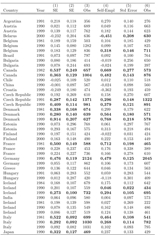
Table 2 reports the estimates of the coe¢ cient for each country and year. It is clear that the self-employed are not always more satis…ed than the employees, but this tends to be the case only in more developed countries. Moreover, the results remain basically unchanged if income is included in the set of controls Xi (columns 4-6). In fact, the set of countries and years in which the self-employed enjoy higher utility becomes slightly larger, which already suggests that income di¤erentials are not the explanation behind di¤erences in job satisfaction.
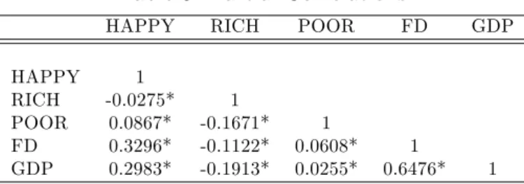
In order to highlight these relationships, we construct the following vari-ables. The variable HAP P Y is a dummy equal to one if is positive and signi…cant at the 5% level. We also run a similar regression with income as dependent variable in equation (13). Given this regression, we construct the dummy RICH which equals one if is positive and signi…cant at the 5% level, and the dummy P OOR which equals one if is negative and signi…cant at the 5% level.
As shown in Table 3, the variable HAP P Y is positively correlated with …nancial development, GDP per capita and P OOR and it is negatively correlated with RICH: In accordance with our model, the self-employed enjoy higher utility than the employees in countries with high GDP per capita and high …nancial development. Moreover, in these countries, the self-employed tend to have a lower income than the employees.
5.2 Job Satisfaction and Financial Development
The previous results suggest that utility di¤erences are not due to …nancial market imperfections. We now explore this argument more systematically. We …rst estimate the equation
Ui;c;t = + Xi;c;t+ Ic;t+ F Dc;t SEi;c;t+ "i;c;t; (14) where Ui;c;t denotes the reported job satisfaction for an individual i in coun-try c and year t; Xi;c;t is a set of individual variables including gender, age, age-squared, education, marital status and employment status; Ic;tis a country-year dummy, F Dc;tis the level …nancial development and SEi;c;t is a dummy equal to one if i is self-employed; …nally, "i;c;t is the error term.11 Equation (14) follows the spirit of Rajan and Zingales (1998), and it allows to estimate the e¤ect of …nancial development on a particular set of individuals, the self-employed, after having controlled for the e¤ect on the whole population and for country-year …xed e¤ects. Our main interest is in the coe¢ cient ; which describes how …nancial development a¤ects the job satisfaction of the self-employed relative to (full-time) employees.12 When is positive, we say that …nancial development is positively correlated with entrepreneurial utility.
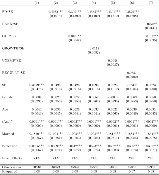
Table 4 reports our estimates on the full sample. The …rst column in-cludes only the controls Xi;c;t. Self-employed, old, married and well-educated individuals tend to be more satis…ed with their job. The second column describes our most basic speci…cation, as reported in equation (14). The coe¢ cient is positive and statistically signi…cant. Financial development bene…ts the self-employed more than the employees.
In order to check the robustness of this result, we …rst try to identify whether …nancial development is capturing any e¤ect of better macroeco-nomic conditions, like better institutions or ecomacroeco-nomic perspectives, which may have a di¤erential impact on the self-employed. When we include GDP per capita, interacted with the employment status dummy, the e¤ect of …nancial development becomes slightly weaker, but still highly signi…cant (column 3). Adding other macroeconomic variables like GDP growth (col-umn 4), unemployment (col(col-umn 5), and an index of regulatory pressure (column 6), always interacted with the self-employment dummy, does not change the estimate of . Hence, our preferred speci…cation, which serves as the baseline for the next analysis, is the one in column (3).
1 1Since these errors may re‡ect common components within countries and employment
status groups, we cluster standard errors at the country/employment status level.
1 2
To ease the interpretation of our coe¢ cients, part-time employees and farmers are excluded from the analysis. These exclusions do not change our results. For the same reason, in what follows, we report the estimates from OLS regressions. The results using ordered probit are qualitatively the same. (see Ferrer-i Carbonell and Frijters, 2004 for a methodological discussion.)
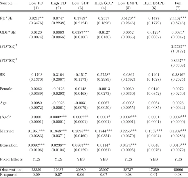
We then check whether this pattern is con…rmed when using an alterna-tive measure of the development of the banking sector, which is a condition for bank credit availability. As in Aghion, Fally and Scarpetta (2007), we employ a variable based on the percentage of bank deposits held in privately owned banks (BANK). The results in column 7 show that also this measure of …nancial development is positively correlated with entrepreneurial utility. Our second set of regressions estimates whether the e¤ect of …nancial development depends on the country’s stage of development. We divide the sample into countries-years with high and with low …nancial development, where such threshold is determined by the median value in our sample.13 The results are in columns (1)-(2) of Table 5: the e¤ects of …nancial de-velopment on entrepreneurial utility are positive and signi…cant only in less developed countries.
Our model suggests a possible explanation for this result. In less de-veloped countries, individuals become self-employed either because of their motivation or for lack of salaried jobs. As these countries develop their …-nancial system, more jobs are created so only those who value it the most remain self-employed. This composition e¤ect is weaker in more developed countries, where labor demand is higher and so most individuals become self-employed by choice. Indeed, we get similar …ndings if we split the sample according to GDP per capita (columns 3-4) or to unemployment (columns 5-6). The e¤ect of …nancial development on entrepreneurial utility is stronger in countries where GDP per capita is low and unemployment is high. Fi-nally, in order to better highlight the nonlinearity in the e¤ects of …nancial development, column (7) includes the level of …nancial development squared and cube. The …rst appears to be negative, the second positive, and both are signi…cant.
From these results, it is evident that the self-employed enjoy higher util-ity than the employees only in countries with high …nancial development; in less developed countries, entrepreneurial utility increase with …nancial development. In highly developed countries, approximately those above the sample median, the e¤ect of …nancial development is U-shaped, and it ap-pears not statistically signi…cant if one applies a linear model.
5.3 Mechanisms
We now explore the mechanisms underlying the relation between …nancial development and entrepreneurial utility. As stressed in our model, these mechanisms should not be evaluated only in monetary terms.
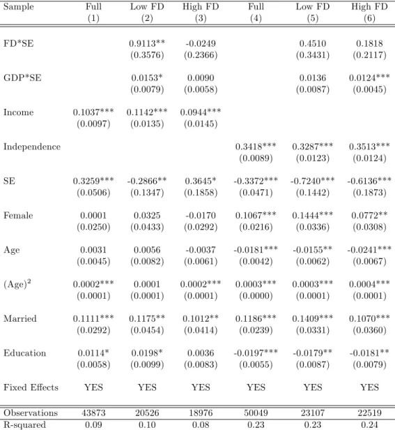
We start by enriching the set of regressors in equation (14). First, we control for income, both in the full sample and separating countries-years according to their level of …nancial development. As shown in columns
(3) of Table 6, if anything, the results are even stronger. Income appears to be a major determinant of job satisfaction; but, as documented also in Benz and Frey (2004), higher income does not explain entrepreneurial utility. In addition to the existing literature, we document that the e¤ects of …nancial development on entrepreneurial utility are not only monetary.14
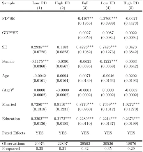
Indeed, by estimating equation (14) with income as dependent variable, we notice that the self-employed are richer than the employees in less de-veloped countries, while this is not the case in more dede-veloped countries (columns 1-2 of Table 7). Moreover, …nancial development decreases the in-come of the self-employed, relative to employees (column 3), and this e¤ect tends to be stronger in less developed countries (columns 4-5). The fact that …nancial development reduces pro…ts is consistent with our model in that …nancial development increases competition, either in the product or in the labor market.
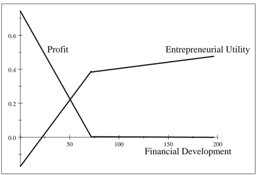
The results in columns (4)-(5) of Table 7 and those in columns (1)-(2) of Table 5 are used to draw Figure 1, which summarizes our main results so far. It clearly emerges that the e¤ects of …nancial development on entrepreneurial utility may di¤er from those on pro…t; actually, in our case, these e¤ects go exactly in the opposite direction. Entrepreneurial utility increases while pro…t decreases with …nancial development, and both e¤ects tend to be stronger in less developed countries.
The above results suggest that …nancial development works through non-monetary aspects of job satisfaction. In the attempt to better identify these mechanisms, we include in our regressions variables like the degree of pride in the work, the satisfaction with job security, the degree of independence enjoyed in the job. We also control for work-related beliefs like how much work is important in life, the main reason why one works, and so on. None of these variables signi…cantly a¤ects our results, with the exception of inde-pendence, that is an indicator derived from the question: "How free are you to make decisions in your job?" The importance of this variable in explaining entrepreneurial utility was already pointed out in Benz and Frey (2004), and indeed, also in our sample, being self-employed becomes negatively related to job satisfaction once one adds this control (Table 6, column 4).
We notice that, once controlling for independence, the e¤ect of …nan-cial development becomes almost half in magnitude and not statistically signi…cant (column 5). Hence, our results add to the existing evidence by documenting that most of the e¤ects of …nancial development seems to work through this channel. According to the model, this is the case since …nan-cial development o¤ers to the most motivated individuals the opportunity to become entrepreneurs. Indeed, these results suggest that what we have
1 4Notice that while income underreporting may be more of an issue for the self-employed,
this may explain our results only if underreporting was higher in more …nancially developed countries.
50 100 150 200 0.0
0.2 0.4 0.6
Profit
Entrepreneurial Utility
Financial Development
Figure 1: Entrepreneurial Pro…t, Utility and Financial Development. Estimates from Table 5, Columns (1)-(2) and Table 7, Columns (4)-(5).
so far called motivation may be (broadly) de…ned in terms of taste for inde-pendence at work. Moreover, notice that the coe¢ cient on indeinde-pendence in less developed countries is lower than in more developed countries (columns 5 and 6).15 This suggests that, as in our model, in more developed country independence is given to those who value it the most.
6
Conclusion and Policy Implications
This paper shows that …nancial development increases utility di¤erences be-tween the self-employed and the employees. This e¤ect is not explained by increased pro…ts; rather, it seems to work through non-monetary dimensions of job satisfaction, and in particular independence. We have interpreted these …ndings by building a simple occupational choice model in which …-nancial development favors both job creation and a better matching between individual motivation and occupation.
We wish to conclude by suggesting some possible policy implications of our analysis. We started by presenting the argument that entrepreneurs enjoy higher utility than employees due to a lack of …nancial development, and showed that such argument is not supported by the data. According to our results, the existence of such utility di¤erences is not due to some market
1 5
imperfection, and as such it does not in itself call for policy intervention. Second, our analysis of utility di¤erences has allowed to formalize the view that self-employment is a rather heterogeneous concept, which indi-viduals may access with very di¤erent motivations. Exploring these moti-vations may be important to understand market behaviors. For example, many self-employed in less …nancially developed countries may view their occupation as temporary, and as such they may be reluctant to invest in long term projects, however e¢ cient these projects may be. Such understanding seems then crucial for assessing entrepreneurs’potential for job creation and growth, and so ultimately for guiding policy interventions.
Finally, we have shown that …nancial development a¤ects also non-monetary dimensions of entrepreneurial utility. This insight suggests that recognizing the importance of entrepreneurs’ intrinsic motivation does not imply that external conditions do not matter. On the contrary, this paper shows how intrinsic motivation is a¤ected by market conditions. A broader investigation on how di¤erent markets and institutions a¤ect non-monetary returns from a job appears a very interesting and highly unexplored avenue for future research.
References
Aghion, P., Fally, T. and Scarpetta, S. (2007), ‘Credit constraints as a barrier to the entry and post-entry growth of …rms’, Economic Pol-icy 22(52), 731–779.
Andersson, P. and Wadensjö, E. (2007), ‘Do the unemployed become suc-cessful entrepreneurs? a comparison between the unemployed, inactive and wage-earners’, International Journal of Manpower 28, 604–626. Banerjee, A. V. and Du‡o, E. (2005), Growth theory through the lens of
development economics, in P. Aghion and S. Durlauf, eds, ‘Handbook of Economic Growth’, Vol. 1 of Handbook of Economic Growth, Elsevier, chapter 7, pp. 473–552.
Banerjee, A. V. and Du‡o, E. (2008), ‘What is middle class about the middle classes around the world?’, Journal of Economic Perspectives 22(2), 3– 28.
Banerjee, A. V. and Newman, A. F. (1993), ‘Occupational choice and the process of development’, Journal of Political Economy 101(2), 274–98. Benz, M. and Frey, B. S. (2004), ‘Being independent raises happiness at
Berner, E., Gomez, G. and Knorringa, P. (2008), ‘Helping a Large Number of People Become a Little Less Poor: The Logic of Survival Entrepre-neurs’, Mimeo. ISS, The Hague.
Bianchi, M. and Henrekson, M. (2005), ‘Is neoclassical economics still en-trepreneurless?’, Kyklos 58(3), 353–377.
Blanch‡ower, D. G. and Oswald, A. J. (1998), ‘What makes an entrepre-neur?’, Journal of Labor Economics 16(1), 26–60.
Borjas, G. J. (1986), ‘The self-employment experience of immigrants’, Jour-nal of Human Resources 21(4), 485–506.
Evans, D. S. and Leighton, L. S. (1989), ‘Some empirical aspects of entre-preneurship’, American Economic Review 79(3), 519–35.
Ferrer-i Carbonell, A. and Frijters, P. (2004), ‘How important is method-ology for the estimates of the determinants of happiness?’, Economic Journal 114(497), 641–659.
Fuchs-Schündeln, N. (2008), ‘On preferences for being self-employed’, Jour-nal of Economic Behavior and Organization Forthcoming.
Glocker, D. and Steiner, V. (2007), ‘Self-employment: A way to end unem-ployment? empirical evidence from german pseudo-panel data’, IZA Discussion Paper No. 2561.
Hamilton, B. H. (2000), ‘Does entrepreneurship pay? an empirical analy-sis of the returns to self-employment’, Journal of Political Economy 108(3), 604–631.
Harris, J. R. and Todaro, M. P. (1970), ‘Migration, unemployment & development: A two-sector analysis’, American Economic Review 60(1), 126–42.
Holmstrom, B. and Tirole, J. (1997), ‘Financial intermediation, loan-able funds, and the real sector’, Quarterly Journal of Economics 112(3), 663–91.
Hundley, G. (2001), ‘Why and when are the self-employed more satis…ed with their work?’, Industrial Relations 40(2), 293–316.
Levine, R. (2005), Finance and growth: Theory and evidence, in P. Aghion and S. Durlauf, eds, ‘Handbook of Economic Growth’, Vol. 1 of Hand-book of Economic Growth, Elsevier, chapter 12, pp. 865–934.
Loayza, N. V. (1994), ‘Labor regulations and the informal economy’, The World Bank Policy Research Working Paper No. 1335.
Moskowitz, T. J. and Vissing-Jorgensen, A. (2002), ‘The returns to entre-preneurial investment: A private equity premium puzzle?’, American Economic Review 92(4), 745–778.
Parker, S. (2004), The Economics of Self-Employment and Entrepreneur-ship, Cambridge University Press.
Rajan, R. G. and Zingales, L. (1998), ‘Financial dependence and growth’, American Economic Review 88(3), 559–86.
Reynolds, P., Bygrave, W., Autio, E., Cox, L. and Hay, M. (2002), Global Entrepreneurship Monitor: 2002 executive report, Babson College. Schneider, F. and Enste, D. H. (2000), ‘Shadow economies: Size, causes,
and consequences’, Journal of Economic Literature 38(1), 77–114. Shapiro, C. and Stiglitz, J. E. (1984), ‘Equilibrium unemployment as a
worker discipline device’, American Economic Review 74(3), 433–44. Taylor, M. P. (1996), ‘Earnings, independence or unemployment: Why
become self-employed?’, Oxford Bulletin of Economics and Statistics 58(2), 253–66.
Weiss, A. W. (1980), ‘Job queues and layo¤s in labor markets with ‡exible wages’, Journal of Political Economy 88(3), 526–38.
7
Appendix
7.1 Omitted Proofs
Lemma 1 The minimal entrepreneurial motivation b is increasing in the share of entrepreneurs x1.
Proof. With simple algebra, di¤erentiating equation (7), one can write @b @x1 = wl (1 x1)2 @p @x1 q:
This expression is positive since the …rst term is positive (notice that x1 may increase only if lx1+ x1 < 1; i.e. there is excess labor supply and w = w, which implies that w does not depend directly on x1) and the second term is negative (Q increases in x1 and so p decreases in x1):
Lemma 2 There exists a level of …nancial development c such that the share of entrepreneurs x1 increases in c for c < c and it is x1= 1=(1+l) for all c c :
Proof. Suppose …rst that lx1+ x1< 1; i.e. there is excess labor supply and w = w: Implicitly di¤erentiating equation (8), we have
@x1 @c = f (a )[1 G(b )] 1 + [1 F (a )]g(b )@x@b 1 :
The numerator measures the increment in individuals who can a¤ord to become entrepreneurs. The denominator tells how the mass of individuals who are su¢ ciently motivated and so willing to be entrepreneurs changes as entry increases. Given Lemma 1, @b =@x1 is positive and hence @x1=@c is also positive. Hence, x1 is strictly increasing in c for lx1+ x1 < 1: Let c be the minimal c such that x1 = 1=(1 + l): Beyond c ; x1 cannot increase any further since everyone is employed either as a worker or as an entrepreneur.
Lemma 3 For c < c ; the price p decreases with c and the wage w is constant at w; for c c ; the price p is constant and the wage w increases with c.
Proof. Given Lemma 2, x1 is strictly increasing in c for c < c : The total output produced Q = x1q depends positively on x1 hence for equation (4) the price p decreases with x1: The wage w instead does not depend on x1; since x1 can increase only if there is excess labor supply and so w = w: For c c ; x1 is …xed and so p is …xed; w instead is such that demand equals
supply of labor, i.e. L = 1 x1 lx1 0: Implicitly di¤erentiating L, we have @w @c = @L @c= @L @w = f (a )[1 G(b )] [1 F (a )]g(b )(1 + l) > 0: Proposition 2
a. Entrepreneurs enjoy higher utility than employees only in more …nan-cially developed countries.
b. Entrepreneurial pro…ts decrease with …nancial development.
c. Entrepreneurial non-monetary bene…ts b increase with …nancial develop-ment, and this e¤ ect may be stronger when …nancial development is low.
Proof. Recall from equation (12) that
U1
lx1 1 x1
U2:
If c is low, then x1 is low and so there are many entrepreneurs for which U1 < U2: These are the individuals with motivation b 2 [b ; b ]; where b is such that + b = w: If c c ; then lx1 = 1 x1 and U1 U2 for all entrepreneurs. Part b. of the Proposition follows from Lemma 3: as c increases, either p decreases or w increases, hence the pro…t = pq wl k decreases with c. Finally, from equation (9), we have
@b @c = g(b ) 1 G(b )(b b ) @b @c:
From equation (7), we see that b increases in x1 and p and it decreases in w so, given Lemmas 1, 2 and 3, @b =@c > 0. This implies that b increases in c: Notice also that this e¤ect may be stronger for c < c ; when b increases in c both as the result of reduced pro…t and of an higher probability of being hired (an higher lx1=(1 x1)). For c c ; instead, only the …rst e¤ect is at play.
7.2 Description of variables
Individual-level variables:
Job Satisfaction: 1-10 index based on the answer to "Overall, how sat-is…ed or dissatsat-is…ed are you with your job?" 10 indicates "satsat-is…ed", 1 indi-cates "dissatis…ed". Source: WVS, variable c033.
SE: Dummy equal 1 if the individual is self-employed. Source: WVS, variable x028.
Female: Dummy equal 1 if the individual is a female. Source: WVS, variable x001.
Age: Age of the individual. Source: WVS, variable x003.
Married: Dummy equal 1 if the individual is married or living together as married. Source: WVS, variable x007.
Education: 1-10 index for the age at which the individual completed education. 1 indicates the individual was less than 13 years old, 10 indicates the individuals was more than 20 years old. Source: WVS, variable x023r.
Income: 1-11 index of the individual income scale. Source: WVS, vari-able x047.
Independence in job: 1-10 index based on the answer to "How free are you to make decisions in your job?" 10 indicates "a great deal", 1 indicates "none at all". Source: WVS, variable c034.
Macro-level variables:
FD: Financial Development, measured by the level of domestic credit to the private sector (% of GDP). Source: World Development Indicators. (available at www.worldbank.org/data)
GDP: GDP per capita (at constant 2000 US$). Source: World Develop-ment Indicators. (available at www.worldbank.org/data)
UNEMPL: Total unemployment (% of total labor force). Source: World Development Indicators. (available at www.worldbank.org/data)
REGULAT: 0-10 variable rating the regulation of credit markets, la-bor markets and businesses. 0 corresponds to stronger state intervention.
Source: Economic Freedom of the World: 2007 Annual Report. (available at www.freetheworld.com)
GROWTH: GDP per capita growth (annual %). Source: World Devel-opment Indicators. (available at www.worldbank.org/data)
BANK: 0-10 variable based on the percentage of bank deposits held in privately owned banks. Countries with larger shares of privately held deposits received higher ratings. Source: Economic Freedom of the World: 2007 Annual Report. (available at www.freetheworld.com)
7.3 Tables
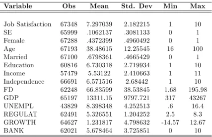
Table 1: Summary Statistics
Variable Obs Mean Std. Dev Min Max
Job Satisfaction 67348 7.297039 2.182215 1 10 SE 65999 .1062137 .3081133 0 1 Female 67288 .4372399 .4960492 0 1 Age 67193 38.48615 12.25545 16 100 Married 67100 .6798361 .4665429 0 1 Education 60816 6.730318 2.719934 1 10 Income 57479 5.53122 2.410663 1 11 Independence 66691 6.571516 2.68442 1 10 FD 62248 66.83599 38.53845 1.68 195.98 GDP 65197 13311.15 9797.721 317 43267 UNEMPL 43829 8.398348 4.252513 .6 16.4 REGULAT 62491 5.326551 1.204252 2.5 8.3 GROWTH 64627 1.231817 4.798632 -14.57 12.67 BANK 62021 5.678464 3.725851 0 10
Note: The table reports summary statistics for all variables used in the regressions. A de…nition of these variables can be found in Section 7.2.
Table 2: Job Satisfaction across countries
(1) (2) (3) (4) (5) (6)
Country Year SE SE Obs Self-Empl Std Error Obs
Argentina 1991 0,218 0,118 356 0,270 0,140 276 Austria 1990 0,021 0,112 689 0,049 0,116 663 Austria 1999 0,139 0,117 762 0,182 0,144 623 Belarus 2000 -0,232 0,204 636 -0,451 0,208 630 Belgium 1981 0,189 0,159 503 0,104 0,185 429 Belgium 1990 0,145 0,080 1282 0,099 0,107 825 Belgium 1999 0,183 0,129 836 0,318 0,146 711 Brazil 1991 0,073 0,097 797 0,092 0,100 764 Bulgaria 1990 0,080 0,186 414 -0,019 0,256 650 Bulgaria 1999 0,078 0,244 693 -0,024 0,199 397 Canada 1982 0,537 0,249 657 0,669 0,277 573 Canada 1990 0,363 0,129 1004 0,482 0,143 876 Chile 1990 -0,025 0,109 520 0,012 0,110 518 China 1990 -0,001 0,097 567 -0,024 0,098 560 Croatia 1999 -0,249 0,180 474 -0,362 0,193 459 Czech Republic 1990 0,192 0,269 610 0,158 0,270 607 Czech Republic 1991 0,287 0,142 1371 0,296 0,148 1322 Czech Republic 1999 0,409 0,114 981 0,379 0,121 891 Denmark 1981 0,338 0,168 674 0,299 0,179 622 Denmark 1990 0,280 0,140 639 0,564 0,180 571 Denmark 1999 0,914 0,207 627 0,768 0,218 578 Estonia 1990 0,073 0,296 768 0,061 0,297 767 Estonia 1999 0,293 0,167 575 0,313 0,218 494 Finland 1990 0,197 0,151 424 -0,022 0,031 424 Finland 2000 0,163 0,148 490 0,222 0,153 449 France 1981 0,500 0,149 588 0,712 0,198 465 France 1990 0,228 0,237 453 0,176 0,338 389 France 1999 0,224 0,227 736 0,166 0,278 610 Germany 1990 0,476 0,119 2124 0,479 0,125 2045 Germany 1999 0,055 0,117 862 0,106 0,173 607 Greece 1999 0,136 0,122 644 0,046 0,134 563 Hungary 1991 0,063 0,283 552 0,059 0,283 544 Hungary 1999 0,012 0,287 420 -0,118 0,301 409 Iceland 1984 0,168 0,107 679 0,175 0,112 642 Iceland 1990 0,201 0,107 559 0,046 0,022 434 Iceland 1999 0,273 0,100 732 0,294 0,105 695 India 1990 0,064 0,096 580 0,004 0,097 573 Ireland 1981 0,198 0,139 598 0,027 0,269 222 Ireland 1990 0,078 0,135 549 0,162 0,148 486 Ireland 1999 0,086 0,127 519 0,124 0,138 461 Italy 1981 0,522 0,092 699 0,464 0,108 541 Italy 1990 0,292 0,092 1030 0,268 0,114 782 Italy 1999 0,092 0,082 1031 0,102 0,093 795 Japan 1990 0,322 0,127 469 0,237 0,133 429
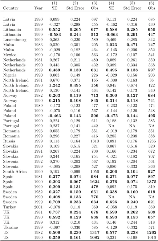
Table 2 continued
(1) (2) (3) (4) (5) (6)
Country Year SE Std Error Obs SE Std Error Obs
Latvia 1990 0,099 0,224 697 0,113 0,224 685 Latvia 1999 -0,327 0,298 455 -0,462 0,316 430 Lithuania 1990 0,552 0,265 677 0,588 0,285 650 Lithuania 1999 -0,583 0,244 513 -0,663 0,291 447 Luxembourg 1999 0,363 0,220 589 0,469 0,285 342 Malta 1983 0,520 0,301 205 1,023 0,471 147 Malta 1999 -0,029 0,182 464 -0,145 0,206 352 Mexico 1990 -0,170 0,106 563 -0,172 0,107 541 Netherlands 1981 0,267 0,211 480 0,089 0,261 350 Netherlands 1990 0,445 0,305 432 0,389 0,334 358 Netherlands 1999 0,489 0,130 631 0,495 0,138 597 Nigeria 1990 0,063 0,149 226 -0,029 0,156 203 North Ireland 1981 0,670 0,371 165 -0,300 0,163 36 North Ireland 1990 1,242 0,495 156 0,945 0,674 122 North Ireland 1999 0,130 0,141 464 0,142 0,173 340 Norway 1982 0,263 0,119 713 0,300 0,127 684 Norway 1990 0,215 0,108 845 0,314 0,118 741 Poland 1989 -0,173 0,122 477 -0,232 0,123 474 Poland 1990 -0,075 0,116 567 -0,144 0,120 548 Poland 1999 -0,463 0,143 506 -0,475 0,144 495 Portugal 1990 0,224 0,129 611 0,188 0,132 585 Portugal 1999 0,237 0,141 442 NA NA NA Romania 1993 0,055 0,179 551 -0,019 0,179 551 Romania 1999 0,296 0,227 416 0,285 0,238 388 Russia 1999 0,113 0,164 1310 0,091 0,176 1235 Slovakia 1990 0,109 0,515 321 0,067 0,516 320 Slovakia 1991 0,267 0,224 708 0,166 0,234 672 Slovakia 1999 0,244 0,165 754 -0,021 0,182 707 Slovenia 1992 0,270 0,202 567 0,192 0,204 561 Slovenia 1999 -0,085 0,208 527 0,080 0,332 366 South Africa 1990 0,192 0,099 1056 0,206 0,104 927 Spain 1981 0,277 0,074 984 0,271 0,077 897 Spain 1990 0,293 0,067 1624 0,276 0,074 1375 Spain 1999 0,299 0,131 478 0,092 0,175 319 Sweden 1982 0,327 0,150 651 0,338 0,160 619 Sweden 1990 0,408 0,133 770 NA NA NA Sweden 1999 0,709 0,233 634 0,626 0,240 621 Turkey 2001 -0,078 0,118 369 -0,058 0,119 369 UK 1981 0,737 0,224 678 0,590 0,262 509 UK 1990 0,592 0,129 838 0,593 0,153 657 UK 1999 0,312 0,210 434 0,146 0,244 318 Ukraine 1999 -0,097 0,330 585 -0,129 0,332 571 US 1982 0,506 0,230 1317 0,577 0,238 1262 US 1990 0,359 0,161 1082 0,321 0,168 1016
Note: This table reports the results of ordered probit regressions of job satisfaction on a dummy equal 1 if the individual is self-employed. Columns (1) and (4) report the estimated coe¢ cients. In columns (1)-(3), the controls are gender, age, age squared, education, marital status. In columns (4)-(6), income is also included in the controls. NA indicates that no observation on income is available for that country in that year. Coe¢ cients signi…cant at the 5% level are reported in bold.
Table 3: Partial Correlations
HAPPY RICH POOR FD GDP
HAPPY 1
RICH -0.0275* 1
POOR 0.0867* -0.1671* 1
FD 0.3296* -0.1122* 0.0608* 1
GDP 0.2983* -0.1913* 0.0255* 0.6476* 1
Note: The table reports partial correlation coe¢ cients. The star indicates signi…cance at the 1% level. HAPPY is a dummy equal 1 if the coe¢ cient on self-employment is positive and signi…cant at the 5% level in a ordered probit re-gression with job satisfaction as dependent variable. RICH is a dummy equal 1 if the coe¢ cient on self-employment is positive and signi…cant at the 5% level in a ordered pro-bit regression with income as dependent variable. POOR is a dummy equal 1 if the coe¢ cient on self-employment is negative and signi…cant at the 5% level in a ordered probit regression with income as dependent variable. All regres-sions include gender, age, age squared, education, marital status as controls.
Table 4: Financial Development and Job Satisfaction: Basic results (1) (2) (3) (4) (5) (6) (7) FD*SE 0.4932*** 0.3091** 0.4535*** 0.4391*** 0.3829*** (0.1074) (0.1390) (0.1109) (0.1310) (0.1308) BANK*SE 0.0278** (0.0141) GDP*SE 0.0101** 0.0103*** (0.0047) (0.0035) GROWTH*SE -0.0112 (0.0082) UNEMP*SE 0.0048 (0.0087) REGULAT*SE 0.0657 (0.0402) SE 0.3679*** 0.0496 0.0426 0.1095 0.0625 -0.2306 0.0823 (0.0478) (0.0910) (0.0916) (0.1015) (0.1519) (0.1984) (0.0900) Female 0.0004 0.0028 0.0077 0.0057 -0.0089 0.0063 0.0050 (0.0233) (0.0253) (0.0258) (0.0261) (0.0295) (0.0253) (0.0250) Age 0.0040 0.0036 0.0026 0.0032 0.0021 0.0036 0.0031 (0.0043) (0.0045) (0.0044) (0.0044) (0.0063) (0.0046) (0.0043) (Age)2 0.0001*** 0.0001*** 0.0002*** 0.0001*** 0.0002** 0.0001*** 0.0002*** (0.0000) (0.0000) (0.0000) (0.0000) (0.0001) (0.0001) (0.0000) Married 0.1870*** 0.1904*** 0.1905*** 0.1905*** 0.1817*** 0.1884*** 0.1854*** (0.0257) (0.0281) (0.0283) (0.0285) (0.0311) (0.0285) (0.0278) Education 0.0305*** 0.0309*** 0.0312*** 0.0323*** 0.0302*** 0.0306*** 0.0307*** (0.0067) (0.0071) (0.0072) (0.0073) (0.0080) (0.0073) (0.0071)
Fixed E¤ects YES YES YES YES YES YES YES
Observations 50510 46873 45996 45550 34836 45855 46353
R-squared 0.08 0.08 0.08 0.08 0.08 0.07 0.08
Note: This table reports the results of OLS regressions with job satisfaction as dependent variable. All regressions include country-year dummies. The coe¢ cient estimates and the standard errors for FD*SE are multiplied by 100. The coe¢ cient estimates and the standard errors for GDP*SE are multiplied by 1000. Robust standard errors, clustered at the country-employment status level, are in brackets. , and denote rejection of the null hypothesis of the coe¢ cient being equal to 0 at 10%, 5% and 1% signi…cance level, respectively.
Table 5: Financial Development and Job Satisfaction: Non-linear e¤ects
Sample Low FD High FD Low GDP High GDP Low EMPL High EMPL Full
(1) (2) (3) (4) (5) (6) (7) FD*SE 0.8217** 0.0747 0.3759* 0.2557 0.5120** 0.1477 2.4467*** (0.3476) (0.2238) (0.2124) (0.1896) (0.2546) (0.1779) (0.8745) GDP*SE 0.0120 0.0063 0.0387*** -0.0127 0.0052 0.0129* 0.0084* (0.0074) (0.0056) (0.0100) (0.0130) (0.0055) (0.0067) (0.0047) (FD*SE)2 -2.5535** (1.0127) (FD*SE)3 0.8337** (0.3308) SE -0.1703 0.3164 -0.1517 0.5758* -0.0362 0.1401 -0.3846* (0.1370) (0.2067) (0.1173) (0.2989) (0.1392) (0.1628) (0.2025) Female 0.0262 -0.0126 0.0148 -0.0013 0.0030 0.0140 0.0072 (0.0389) (0.0293) (0.0468) (0.0273) (0.0360) (0.0352) (0.0260) Age 0.0080 -0.0026 -0.0031 0.0067 -0.0003 0.0064 0.0025 (0.0072) (0.0061) (0.0079) (0.0050) (0.0055) (0.0085) (0.0044) (Age)2 0.0001 0.0002*** 0.0002** 0.0001* 0.0002*** 0.0001 0.0002*** (0.0001) (0.0001) (0.0001) (0.0001) (0.0001) (0.0001) (0.0000) Married 0.1951*** 0.1848*** 0.2095*** 0.1744*** 0.2255*** 0.1332*** 0.1902*** (0.0383) (0.0371) (0.0460) (0.0354) (0.0370) (0.0404) (0.0283) Education 0.0392*** 0.0238** 0.0563*** 0.0114* 0.0474*** 0.0048 0.0313*** (0.0106) (0.0104) (0.0129) (0.0061) (0.0095) (0.0076) (0.0072)
Fixed E¤ects YES YES YES YES YES YES YES
Observations 23359 22637 20989 25007 28737 17259 45996
R-squared 0.09 0.07 0.06 0.07 0.08 0.07 0.08
Note: This table reports the results of OLS regressions with job satisfaction as dependent variable. All regressions include country-year dummies. In columns (1)-(2), Low FD and High FD indicate that the sample is restricted to countries respectively below and above the median value of FD in our sample (equal to 71.78). Similarly, in columns (3)-(4), Low GDP and High GDP indicate that the sample is restricted to countries respectively below and above the median value of GDP in our sample (equal to 11,346); and in columns (5)-(6), Low EMPL and High EMPL indicate that the sample is restricted to countries respectively above and below the median value of UNEMPL in our sample (equal to 8.2). The coe¢ cient estimates and the standard errors for FD*SE are multiplied by 100. The coe¢ cient estimates and the standard errors for GDP*SE are multiplied by 1000. Robust standard errors, clustered at the country-employment status level, are in brackets. , and denote rejection of the null hypothesis of the coe¢ cient being equal to 0 at 10%, 5% and 1% signi…cance level, respectively.
Table 6: Financial Development and Job Satisfaction: Mechanisms
Sample Full Low FD High FD Full Low FD High FD
(1) (2) (3) (4) (5) (6) FD*SE 0.9113** -0.0249 0.4510 0.1818 (0.3576) (0.2366) (0.3431) (0.2117) GDP*SE 0.0153* 0.0090 0.0136 0.0124*** (0.0079) (0.0058) (0.0087) (0.0045) Income 0.1037*** 0.1142*** 0.0944*** (0.0097) (0.0135) (0.0145) Independence 0.3418*** 0.3287*** 0.3513*** (0.0089) (0.0123) (0.0124) SE 0.3259*** -0.2866** 0.3645* -0.3372*** -0.7240*** -0.6136*** (0.0506) (0.1347) (0.1858) (0.0471) (0.1442) (0.1873) Female 0.0001 0.0325 -0.0170 0.1067*** 0.1444*** 0.0772** (0.0250) (0.0433) (0.0292) (0.0216) (0.0336) (0.0308) Age 0.0031 0.0056 -0.0037 -0.0181*** -0.0155** -0.0241*** (0.0045) (0.0082) (0.0061) (0.0042) (0.0062) (0.0067) (Age)2 0.0002*** 0.0001 0.0002*** 0.0003*** 0.0003*** 0.0004*** (0.0001) (0.0001) (0.0001) (0.0000) (0.0001) (0.0001) Married 0.1111*** 0.1175** 0.1012** 0.1186*** 0.1409*** 0.1070*** (0.0292) (0.0454) (0.0414) (0.0239) (0.0331) (0.0360) Education 0.0114* 0.0198* 0.0036 -0.0197*** -0.0179** -0.0181** (0.0058) (0.0099) (0.0083) (0.0055) (0.0087) (0.0079)
Fixed E¤ects YES YES YES YES YES YES
Observations 43873 20526 18976 50049 23107 22519
R-squared 0.09 0.10 0.08 0.23 0.23 0.24
Note: This table reports the results of OLS regressions with job satisfaction as dependent variable. All regressions include country-year dummies. Low FD and High FD indicate that the sample is restricted to countries respectively below and above the median value of FD in our sample (equal to 71.78). The coe¢ cient estimates and the standard errors for FD*SE are multiplied by 100. The coe¢ cient estimates and the standard errors for GDP*SE are multiplied by 1000. Robust standard errors, clustered at the country-employment status level, are in brackets. , and denote rejection of the null hypothesis of the coe¢ cient being equal to 0 at 10%, 5% and 1% signi…cance level, respectively.
Table 7: Financial Development and Income
Sample Low FD High FD Full Low FD High FD
(1) (2) (3) (4) (5) FD*SE -0.4107** -1.3760*** -0.0027 (0.1956) (0.3989) (0.4473) GDP*SE 0.0027 0.0087 0.0022 (0.0059) (0.0084) (0.0094) SE 0.2935*** 0.1183 0.4228*** 0.7426*** 0.0473 (0.0728) (0.0823) (0.1082) (0.1273) (0.3842) Female -0.1175*** -0.0391 -0.0625 -0.1222*** 0.0063 (0.0360) (0.0567) (0.0395) (0.0369) (0.0642) Age -0.0042 0.0094 0.0071 -0.0046 0.0202 (0.0161) (0.0164) (0.0139) (0.0163) (0.0193) (Age)2 0.0000 -0.0000 -0.0001 0.0000 -0.0002 (0.0002) (0.0002) (0.0002) (0.0002) (0.0002) Married 0.7280*** 0.9110*** 0.8770*** 0.7369*** 1.0272*** (0.1318) (0.1231) (0.0960) (0.1312) (0.1270) Education 0.2202*** 0.2172*** 0.2289*** 0.2214*** 0.2373*** (0.0136) (0.0185) (0.0110) (0.0137) (0.0199)
Fixed E¤ects YES YES YES YES YES
Observations 20976 22897 39502 20526 18976
R-squared 0.35 0.31 0.32 0.35 0.29
Note: This table reports the results of OLS regressions with income as de-pendent variable. All regressions include country-year dummies. Low FD and High FD indicate that the sample is restricted to countries respectively below and above the median value of FD in our sample (equal to 71.78). The co-e¢ cient estimates and the standard errors for FD*SE are multiplied by 100. The coe¢ cient estimates and the standard errors for GDP*SE are multiplied by 1000. Robust standard errors, clustered at the country-employment status level, are in brackets. , and denote rejection of the null hypothesis of the coe¢ cient being equal to 0 at 10%, 5% and 1% signi…cance level, respectively.