Imputation of income variables in a survey context and estimation of variance for indicators of poverty and social exclusion

PhD Thesis submitted to the Faculty of Economics and Business

Institute of Statistics

University of Neuchâtel

For the degree of PhD in Statistics

by

Eric GRAF

Accepted by the dissertation committee:

Prof. Yves TILLÉ, University of Neuchâtel, thesis director

Prof. Catalin STARICA, University of Neuchâtel, jury president

Dr. Camelia GOGA, HDR, University of Bourgogne, France

Dr. Jean-Pierre RENFER, Swiss Federal Office of Statistics

Prof. Louis-Paul RIVEST, University of Laval, Canada

Defended on 3

rd

of November 2014

IMPUTATION OF INCOME VARIABLES IN A SURVEY

CONTEXT AND ESTIMATION OF VARIANCE FOR

INDICATORS OF POVERTY AND SOCIAL EXCLUSION

Faculté des Sciences Economiques Avenue du 1er-Mars 26

CH-2000 Neuchâtel

Acknowledgements

T

hiswork is funded and was carried out under a productive collabora-tion agreement between the Swiss Federal Office of Statistics (SFSO) and the Institute of Statistics (ISTAT) at the University of Neuchâtel. Let both parties being warmly thanked here. Let Pr. Yves Tillé be thanked here for the opportunity, the privilege and also the pleasure of working with him. I always found great support over the past three years when-ever I needed it. Let the Section of Methods (METH) and the Section of Income, Consumption and Living Conditions (EKL) of the SFSO also be thanked. Particularly I want to express my great gratitude to Dr. Philippe Eichenberger and Dr. Jean-Pierre Renfer from METH because they agreed and supported me in quitting my methodologist position at the SFSO in favour of transfer to ISTAT in order to produce this thesis. I have ex-tensively benefited from my working experience of nearly 9 years at the SFSO and also at the Swiss Household Panel (SHP) for the time it was still based at the University of Neuchâtel. The problems I encountered during these years of service and how they were solved really gave birth to my inspiration to pursue this thesis. I sincerely thank Pr. Catalin Star-ica who accepted to be the president of this jury, Pr. Louis-Paul RIVEST, Dr. Camelia Goga and Dr. Jean-Pierre Renfer who accepted to review this document. It is a great honour for me. Thanks also go to my colleagues and former colleagues, at the University of Neuchâtel, the SFSO and the SHP. I always had good contacts with them and I learnt a lot with them. Finally, I wish to thank my whole family and my friends who gave me support and encouragement.

Neuchâtel, 28 August 2014.

Contents

Contents 9

List of Figures 13

List of Tables 15

Introduction 23

1 The SILC survey in Switzerland 27

1.1 Sampling design and weighting scheme . . . 27

1.2 Variable of interest for development of an imputation strategy . . . 29

2 Sondage dans des registres de population et de mé-nages en Suisse : coordination d’enquêtes, pondéra-tion et imputapondéra-tion 31 2.1 Introduction . . . 32

2.2 Les différentes enquêtes auprès de la population des personnes et des ménages résidant enSuisse . . . 33

2.2.1 Le nouveau système de recensement de la population suisse 33 2.2.2 Les enquêtes sur les conditions de vie, le budget des mé-nages et la population active . . . 35

2.3 Enquêtes coordonnées dans le fichier SRPH . . . 36

2.3.1 Coordination d’échantillons . . . 37

2.3.2 Algorithme d’échantillonnage coordonné . . . 39

2.3.3 Sélection d’une seule personne par ménage . . . 45

2.4 Estimation et Pondération . . . 48

2.4.1 Calcul des probabilités d’inclusion . . . 48

2.4.2 Calcul de probabilités de réponse . . . 51

2.4.3 Calage. . . 54

2.4.4 Poids partagés et poids combinés . . . 57

2.5 Traitement des données et imputation . . . 59

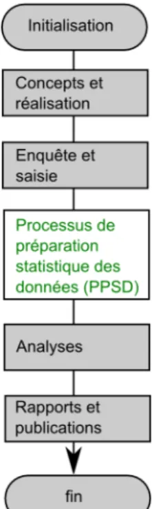
2.5.1 Processus de préparation statistique des données. . . 60

2.5.2 Non-réponse . . . 61

2.5.3 Valeurs erronées et valeurs aberrantes . . . 63

2.5.4 Imputations . . . 64

2.6 Estimation de variance . . . 67

2.6.1 Pour le relevé structurel et les autres enquêtes sélection-nées de manière coordonnée dans le fichier SRPH . . . . 67

2.7.2 Sur l’estimation de la variance due à l’imputation . . . . 70

2.7.3 Sur la sélection des échantillons pour les enquêtes de l’OFS dans un avenir proche . . . 70

2.8 Conclusions . . . 71

3 Variance Estimation Using Linearization for Poverty andSocial Exclusion Indicators 73 3.1 Introduction . . . 73

3.2 Review of given poverty indicators and their lin-earized variables . . . 74

3.2.1 Gini coefficient . . . 77

3.2.2 Quintile Share Ratio (QSR or S₈₀/S₂₀) . . . 78

3.2.3 Linearized variable of a quantile. . . 79

3.2.4 Median income and at-risk-of-poverty threshold . . . 80

3.2.5 At Risk of Poverty Rate . . . 80

3.2.6 Median income of individuals below the ARPT. . . 81

3.2.7 Relative Median Poverty Gap . . . 81

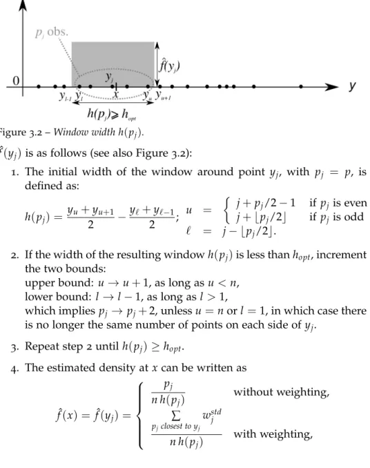
3.3 Estimating the income density function . . . 81

3.3.1 Using the logarithm . . . 82

3.3.2 Nearest neighbour with minimum bandwidth . . . 83

3.3.3 Robustness of the linearized variable . . . 85

3.4 Results . . . 85

3.5 Conclusions . . . 89

4 Variance Estimation for Regression Imputed Quan-tiles: A first step towards Variance Estimation for Regression Imputed Inequality Indicators 91 4.1 Introduction . . . 92

4.2 Notations . . . 93

4.3 Variance due to multiple regression imputation . . . . 94

4.3.1 Goal: obtain a confidence interval for the total Y . . . 94

4.3.2 Sampling variance: ˆV_sam . . . 96

4.3.3 Imputation variance: ˆV_imp . . . 97

4.3.4 Total variance: ˆV_tot . . . 98

4.4 Variance of inequality indicators . . . 99

4.4.1 Degree of a functional . . . 100

4.5 Total variance for quantiles . . . 101

4.5.1 Linearized variable of a quantile. . . 101

4.5.2 Sampling variance: ˆV_sam . . . 101

4.5.3 Imputation variance: ˆV_imp . . . 105

4.5.4 Total variance for the linearized variable of a quantile . . 106

4.6 Simulations from real data . . . 106

4.6.1 Simulations: employees’ income SILC09. . . 109

4.7 Results . . . 110

4.7.2 Components of total variance in the case of quantiles . . 111

4.7.3 Biais of estimators . . . 112

4.8 Conclusions . . . 115

4.9 Acknowledgements . . . 116

5 Imputation of income data with generalized calibra-tion procedure and GB2 distribution: illustration withSILC data 117 5.1 Introduction . . . 118

5.2 Notations . . . 119

5.3 GB2 distribution and fit . . . 121

5.4 Generalized calibration . . . 121

5.4.1 Instrumental variable regression . . . 123

5.4.2 Choosing the auxiliary and instrumental variables . . . . 127

5.5 Ranks, robustness and normal scores . . . 128

5.5.1 Weighted ranks . . . 128

5.5.2 Normal scores . . . 129

5.6 Imputation strategy . . . 129

5.7 Estimating the variance . . . 130

5.8 Real data application . . . 133

5.8.1 Segmentation . . . 133

5.8.2 Detailed imputation procedure . . . 134

5.8.3 Results . . . 139 5.9 Conclusion . . . 144 5.10 Acknowledgement . . . 146 6 Discussion 147 6.1 Notes on the GB2 . . . 147 6.1.1 GB2 distribution function . . . 148

6.1.2 Moments of the GB2 distribution . . . 148

6.1.3 Indicators of poverty and social exclusion in the EU-SILC and GB2 Distribution. . . 149

6.1.4 Note on the variance-covariance matrix of totals of the GB2 estimated scores . . . 151

6.2 Some remarks about the Durbin-Wu-Hausman test . . . 152

6.2.1 DWH tests with weighted observations . . . 155

6.2.2 Lessons learned so far with DWH tests . . . 157

General conclusion 159

A Proof of Proposition 4.3 161

B Proof of Proposition 4.4 165

C Expression for CQα,sas ₁₆₇

D Definition of the variables used 169

List of Figures

1.1 Employee’s income collected by CATI versus CCO-register

value. . . 30

2.1 Zone de sélection pour la première enquête. . . 40

2.2 Coordination positive, avecπ2 k ≤π1k. . . 41

2.3 Coordination négative lorsqueπ1 k+π2k ≤1. . . 41

2.4 Coordination négative lorsqueπ1 k+π2k ≥1. . . 41

2.5 Coordination d’un troisième échantillon. . . 42

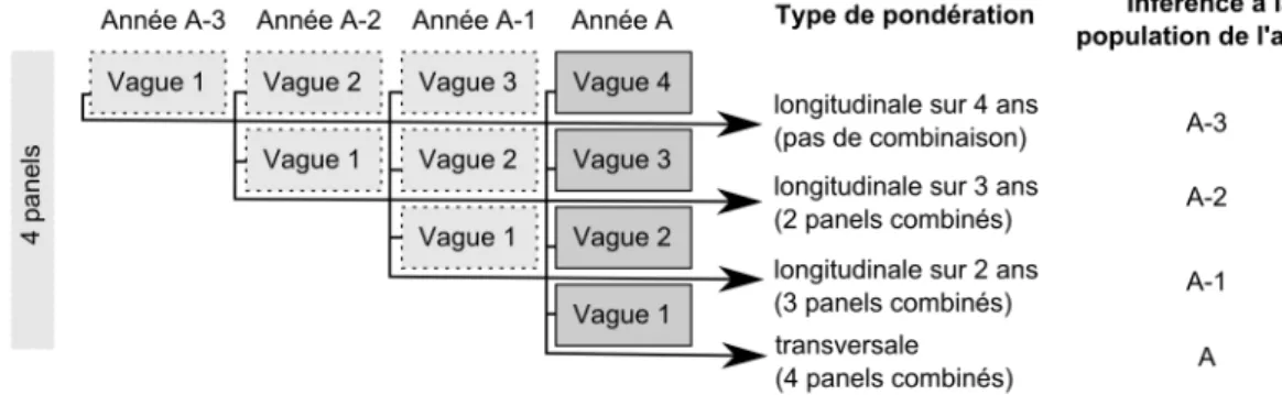
2.6 Plan rotatif de l’enquête SILC. . . 59

2.7 Schéma d’enquête. . . 60

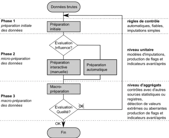
2.8 Processus de préparation statistique des données. . . 61

3.1 Gini coefficient, G, and Lorenz curve L(α). G = 2A, A+ B=1/2. . . 78

3.2 Window width h(p_j). . . 84

4.1 Descriptive statistics of the population used for the sim-ulations (employees’ income smaller than 200’000.- Swiss Francs, SILC09): kernel estimated density function with the R function drvkde from package feature. . . 108

5.1 Step 1: Income densities and GB2-fits. Left panel, compar-ison between the data and the GB2-fits. Right panel, GB2 fits using weights from generalized calibration with dif-ferent calibration functions: truncated (bounds=0,10), logit (bounds=0,10) and raking ratio. . . 138

5.2 Results. Top panel: income empirical densities. Mid-dle left panel: quantiles of the absolute imputation er-ror which corresponds to the real value minus the im-puted value, yCCO,k− ˆyimp,k, k ∈ o. Middle right and two bottom panels, quantiles of the relative imputation error, (yCCO,k− ˆyimp,k)/yCCO,k, k ∈ o; bottom left, zoom on origi-nal income below 20,000.-, bottom right, zoom on origiorigi-nal income over 20,000.- CHF. . . 142

ing observation. Top panels: income empirical densities. Four lower panels: quantiles of the absolute, yCCO,k− ˆyimp,k,

(middle ones) and relative, (yCCO,k − ˆyimp,k)/yCCO,k, k ∈ o

(bottom ones) imputation error, k∈o. . . 143

6.1 Links between the GB2 and other well-known distributions. 147 E.1 Segmentation tree first part. Refer to Table D.1 for the

defi-nitions of variables. . . 171 E.2 Segmentation tree second part. Refer to Table D.1 for the

List of Tables

1.1 Detailed nonresponse affecting employee personal income, CATI-variable. (NR = nonresponse, I.Q. = individual ques-tionnaire, F_cati = nonresponse flag for variable yCATI).

Nonresponse affecting the corresponding register variable (due to the failure of matching) is also detailed (F_cco = nonresponse flag for variable ycco). . . 29 1.2 Descriptives statistics of employee’s income, CCO-variable,

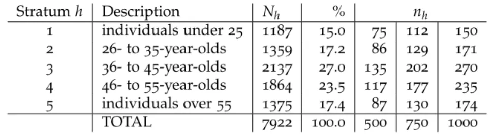
depending on the reasons for nonresponse to CATI. . . 30 3.1 Strata used in simulations with 2009 EU-SILC data and

three sample sizes (income of salaried individuals, N =7, 922) 86 3.2 Calibration margins in simulations with 2009 EU-SILC data

(income of salaried individuals, N =7, 922) . . . 87 3.3 Relative bias (3.8) of the variance obtained with 10,000

sim-ple random samsim-ples without replacement from the 2009 EU-SILC data (equivalent household income, N =17, 534) . . . 87 3.4 Relative bias (3.8) of the variance obtained with 10,000

sim-ple random samsim-ples without replacement from the 2009 EU-SILC data (income of salaried individuals, N =7, 922) . . . 88 3.5 Relative bias (3.8) of the variance obtained with 10,000

sim-ple random samsim-ples without replacement from Ilocos data (household income, N=632) . . . 88 3.6 Relative bias (3.8) of the variance obtained with 10,000

strat-ified random samples without replacement, with weights calibrated to eight sociodemographic margins, from the 2009 EU-SILC data (income of salaried individuals, N = 7, 922). . . 89 4.1 Descriptive statistics of the population used for the

simula-tions presented (employees’ income, SILC09), the distribu-tion has been cut to 200,000 Swiss francs to avoid problems due to extreme values. . . 107

out NR. C1: weighted samples but without modeling the NR. C2: weighted samples with weights modeling the NR. D1: imputed samples but imputation ignored. D2: imputed samples, plug-in method Deville & Särndal. D3: imputed samples, our method. . . 111 4.3 Estimated proportions of the various components of the

to-tal variance, see (4.27), V_totQα for the simulation on the em-ployee’s income from SILC 2009. The four components are: the design variance ignoring imputation, Vp(Zˆ•Qα), the

cor-rective term ˆCQα_{, see (4.24), the imputation variance Vimpξ,} see Proposition 4.4, and minus the squared bias ˆB_ξpq(Zˆ•Qα),

see (4.25). . . 112 4.4 Relative biases of the point estimates for the different

vari-ants with the simulations conducted on employee’s income in SILC 2009. B: samples without NR. C1: weighted sam-ples but without modeling NR. C2: weighted samsam-ples with weights modeling the NR. D: imputed samples. . . 114 4.5 Mean Monte-Carlo biases and estimated average bias

ˆB_{ξ pq}(ZˆQ•α) (bias through linearization) on the 2,000

sim-ulations for the three quantiles. . . 114 5.1 Post-control of the generalized calibration by adjusting

cor-responding WIV-regression model and comparing it with a WLS-model. x·j = auxiliary variables known on s, ˆBrzx =

estimated parameters through WIV-regression using the z_·j,

known at least on r, as instruments. ˆBr =estimated

param-eters through WLS, i.e. all x_·j instrumented by themselves. corr(eg, x·j) = correlations between the observed x·j, on r,

and the residuals of the adjusted WIV-regression (biserial correlation if x_·j dichotomous). corr(er, x·j) = correlations

between the observed x_·j, on r, and the residuals of the

ad-justed WLS-regression. corr(eg, z_·j) = correlations between

the observed z_·j, on r, and the residuals of the adjusted

WIV-regression. The 5th and 7th columns reflect the test of con-dition (i), see Section 5.4.1. Note that n−12

r =0.013. . . 136

5.2 Weights for y

CCO, on r, before and after calibration. The

5.3 Imputation-variance estimation from our imputation strat-egy. One can see that the imputation variance is very low compared to the other component, reaching at the maximum 6.6% of the total variance for the RMPG. EMP R + IMP = empirical estimation on respondents + non-respondents imputed by our imputation procedure (origi-nal survey weights). . . 140 5.4 Inequality indicators. All the estimations are weighted. 95%

confidence estimated intervals. EMP ALL = empirical esti-mation on all the individuals (no nonresponse, original sur-vey weights), EMP R = empirical estimation on respondents only (original survey weights, no nonresponse correction), EMP R Gen Calib = empirical estimation on respondents only using weights stemming from the generalized cali-bration, GB2 ALL = parametric estimation out of the GB2 fitted on all individuals (no nonresponse, original survey weights), GB2 R Gen Calib = parametric estimation out of the GB2 fitted on the respondents only using weights stem-ming from the generalized calibration, GB2 R = parametric estimation out of the GB2 fitted on the respondents using only the original survey weights (no nonresponse correc-tion), EMP R + IMP = empirical estimation on respondents + non-respondents imputed by our imputation procedure (original survey weights). All variance estimations are done through linearization techniques (see Section 5.7) and take the sampling design, several nonresponse corrections, panel combinations and calibrations into account. The variance due to imputation is evaluated through multiple imputa-tion. . . 141 D.1 The first column lists the variables at our disposal, the x_·j

-column is hooked if the variables were retained as auxiliary variables. Similarly the z·j-column is hooked if they were

retained as instrumental variables. The variables with an as-terisk are continuous, all others are dichotomic. The fourth column is hooked if the variables appear in the segmenta-tion tree (see Appendix E) modelling nonresponse. The last column is hooked if the variable correlates at least to 10% with the interst variable yCCO. . . 169

Abstracts

Imputation of income variables in a survey context and estima-tion of variance for indicators of poverty and social exclusion

Keywords : imputation, linearization, weighting, variance, general-ized calibration, GB2.

Abstract

This Phd thesis proposes to develop a method of imputation for in-come variables allowing direct analysis of the distribution of such data, particularly the estimation of complex statistics such as indicators for poverty and social exclusion as well as the estimation of their precision.

In an introduction chapter we present the Swiss Survey on Income and Living Conditions (SILC) which we extensively used to illustrate our research.

In a first article accepted for publication, co-written with Dr. Lionel Qualité, we present an overview of the production methods at the Swiss Federal Office of Statistics (SFSO). Samples are selected with coordination so as to spread the survey burden over the population. We present the computation of extrapolation weights adapted to different cases and needs with its main steps. The SFSO relies on international recommendations for data editing and imputation, and contributes to their elaboration. The precision of estimators is consistently evaluated, according to the different treatments and methods involved in their construction.

In a second published article, co-written with Pr. Yves Tillé, we have used the generalized linearization technique based on the concept of in-fluence function, as Osier (2009) has done, to estimate the variance of com-plex statistics such as Laeken indicators. Through simulations, we show that the use of Gaussian kernel estimation to estimate an income density function results in a strongly biased variance estimate. We propose two other density estimation methods that significantly reduce the observed bias.

In a working paper, we resume the idea presented by Deville & Särndal (1994) which consists in constructing an unbiased estimator of the vari-ance of a total based solely on the information at our disposal (i.e. on the selected sample and the subset of respondents) in the case of regression imputation. While these authors dealt with a conventional total of a vari-able of interest, we reproduce a similar development in the case where the considered total is one of the linearized variable of quantiles. We show by means of simulations on real survey data that regression imputation can have an important impact on the bias and variance estimations of social inequality indicators. This leads us to a method capable of taking into account the variance due to imputation in addition to the one due to the sampling design in the cases of quantiles.

In a submitted article, we present our new imputation method for in-come variables. Empirical studies have shown that the generalized beta distribution of the second kind (GB2) fits income data very well. We present a parametric method of imputation relying on weights stemming from generalized calibration. A GB2 distribution is fitted on the income distribution in order to determine whether these weights can compensate even for nonignorable nonresponse that affects the variable of interest. The success of the operation greatly depends on the choice of auxiliary and in-strumental variables used for calibration, which we discuss. We validate our imputation system on SILC data and compare it to imputations per-formed through the use of IVEware software. We have made great efforts to estimate variances through linearization, taking all the steps of our pro-cedure into account.

The last part of this Phd thesis discusses additional material which we could not include in the other chapters. Namely we give some more in-sights into the GB2 distribution, study the possibility of using Durbin-Wu-Hausman tests in the framework of generalized calibration and present a way of forming imputation classes for an income variable.

Imputation de variables de revenu provenant d’enquête et es-timation de variance pour des indices de pauvreté et d’exclusion sociale

Mots-clés : imputation, linéarisation, pondération, variance, calage généralisé, GB2.

Résumé

Cette thèse développe une méthode d’imputation pour des données de revenus permettant des analyses directes sur la distribution de ces vari-ables et également l’estimation de statistiques complexes telles que des indices de pauvreté et d’exclusions sociale ainsi que l’estimation de leur précision.

Dans un chapitre introductif, nous présentons l’enquête sur les revenus et conditions de vie (SILC) dont les données sont utilisées à plusieurs reprises pour illustrer nos recherches.

Dans un premier article accepté pour publication, co-écrit avec Dr. Lionel Qualité, nous présentons un aperçu des méthodes actuellement utilisées à l’Office Fédéral de la Statistique (OFS). Les échantillons sont sélectionnés de manière coordonnée afin de répartir au mieux la charge d’enquête sur les ménages et les personnes. Le calcul des pondérations, dont on présente les principales étapes, est adapté aux différents besoins et aux différentes situations rencontrées. L’Office se base sur les recomman-dations internationales, dont il participe à l’élaboration, pour le traitement des données d’enquête et les imputations. La précision des estimateurs est systématiquement évaluée en tenant compte des traitements réalisés.

Dans un deuxième article publié, co-écrit avec le Pr. Yves Tillé, nous avons mis en oeuvre la technique de linéarisation généralisée reposant sur le concept de fonction d’influence, tout comme l’a fait Osier (2009),

Abstracts 21

pour estimer la variance de statistiques complexes telles que les indices de Laeken. Des simulations montrent que, pour les cas où l’on a recours à une estimation par noyau gaussien de la fonction de densité des revenus considérés, on obtient un fort biais pour la valeur estimée de la variance. On propose deux autres méthodes pour estimer la densité qui diminuent fortement le biais constaté.

Dans un rapport de recherche, nous résumons l’idée proposée par Deville & Särndal (1994) consistant à construire un estimateur non biaisé de la variance d’un total basé uniquement sur l’information à disposition (c’est-à-dire l’échantillon sélectionné et le sous-ensemble des répondants) dans le cas d’une imputation par régression. Alors que ces auteurs ont traité le total conventionnel d’une variable d’intérêt, nous reproduisons un développement similaire dans le cas où le total considéré est celui de la variable linéarisée d’un quantile. Nous montrons à l’aide de simula-tions sur des données d’enquête réelles que l’imputation par régression peut avoir un impact important sur le biais de la variance estimée pour des indicateurs d’inégalité sociale. Cela nous mène à une méthode capa-ble de prendre en compte la variance due à l’imputation, en plus de celle du plan dans le cas de quantiles.

Dans un article soumis, nous présentons notre nouvelle méthode d’imputation pour des variables de revenus. Des études empiriques ont montré que la loi bêta généralisée de seconde espèce (GB2) s’ajuste très bien à des données monétaires. Nous présentons une méthode d’imputation paramétrique reposant sur l’utilisation de poids issus d’un calage généralisé. Une loi GB2 est ajustée sur la distribution des revenus pour valider ces poids capables de compenser même pour de la non-réponse non-ignorable. Le succès de l’opération dépend grandement du choix, qui est discuté, des variables auxiliaires et instrumentales utilisées pour le calage. Nous validons notre système d’imputation sur les données SILC et comparons les résultats avec ceux obtenus par des imputations réalisées avec le logiciel IVEware. Nous avons investi de gros efforts pour estimer les variances par linéarisation, en prenant toutes les étapes de la procédure en compte.

La dernière partie de la thèse discute du matériel additionnel qui n’a pas pu être inclus dans les autres chapitres. Nous donnons notamment quelques détails supplémentaires sur la distribution GB2, étudions la pos-sibilité d’utiliser des tests de Durbin-Wu-Hausman dans le cadre du calage généralisé et présentons une façon de former des classes d’imputation pour une variable de revenu.

Introduction

U

ndoubtedly, knowledge about income distribution of the population is of vital interest to all studies of economic markets in order to gov-ern economic and social decision-making. In economics and social statis-tics, the study of income distribution is at the heart of inequality measures and more generally of evaluations of social welfare.

In official national sample surveys of households and individuals, non-response in income variables is often a difficult and important problem in the sense that the phenomenon affects the image of the reality that the survey reflects. Without proper treatment, the outcomes of political or social decision-making based on the results of the survey may be wrong.

The initial motivation for this thesis was to attempt to improve the methodology of imputations used at the SFSO for income variables in two of its main surveys, namely the Survey on Income and Living Conditions (SILC) and the Swiss Labour Force Survey (SLFS). Indeed the author of this dissertation played an active role for almost three years developing and adapting acceptable imputations for these surveys. Most of the well-known methods were tested and the main concern was systematically how to adapt the theory to practice in a defensible, reasonable, documentable and reproducible manner.

Typically, the survey methodologist is given a survey-data file contain-ing misscontain-ing values. His mission is to compute survey-weights, imputa-tions or set up a variance estimation methodology for some given statis-tics. A conscientious person cannot be content with accomplishing such a task without obtaining information about what has been done at all stages of the Data Preparation Process (DPP, see Section 2.5.1) for this particular study. For example, we had noticed that the number of phone calls needed during the fieldwork to establish a first contact with a household in Com-puter Assisted Telephone Interview (CATI) surveys was a very important piece of information when modelling nonresponse at several levels of the data collection as well as when imputing missing data. Another example is that the treatment of outliers (in the sense of Chambers, 1986; Hulliger, 1999) or extreme values in the initial phase of the DPP (see Figure 2.8, Sec-tion 2.5.1) can have a major impact on computed weights or imputaSec-tions afterwards. To illustrate this point, sometimes policy decisions have to be met: if the richest person of Switzerland is randomly selected for part of the sample, that person’s fortune (over 35 billion of Swiss Francs1

) is thou-sands of times the median fortune of the Swiss individual or household (around 350,000 SFR, see Müller, 2014). In the fortune distribution, the

1

See BILAN journal, http://www.bilan.ch/300plusriches.

person will be a representative outlier as defined by Chambers (1986); Hul-liger (1999). Such an observation can have a huge and undesired effect on a regression model for example, although it is a true and correctly mea-sured unit. In such cases, the usual treatment is to put aside the influence of that observation or to reduce it, nevertheless without erasing it from the data file.

Red path and motivation

My thesis has been driven by the desire to explore the potential of a new imputation procedure for income variables which would perform better than IVEware (Raghunathan et al., 2001) software that I extensively used for imputations tasks in my work at the SFSO. In this sense, Chapter 5 represents the heart of my work.

Chapter 1 is a short introduction to the Swiss SILC 2009 survey data survey since the following chapters often use an extract of the data orig-inating from this survey to illustrate our different research. It allows the reader to gain more insights about the nature of the dataset. We also ex-plain how the data stemming from the CATI survey could be matched with a register providing exceptional possibilities for methodological re-search.

Chapter 2, which is co-written with Dr. Lionel Qualité, reproduces an article which was reviewed and accepted for publication in a special issue of the Journal de la Société Française de Statistiques. We present an overview of the production methods at the SFSO. Samples are selected with coordination so as to spread the survey burden over the population. We present the computation of extrapolation weights adapted to different cases and needs with its main steps. The SFSO relies on international rec-ommendations for data editing and imputation, and contributes to their elaboration. The precision of estimators is consistently evaluated, accord-ing to the different treatments and methods involved in their construction. This chapter can be considered as an extension of the introduction since it describes the framework in which this thesis is rooted. In the following chapters the reader is considered to be familiar with the notations and issues presented in Chapter 2.

Chapter 3, co-written with Pr. Yves Tillé, reproduces an article which was published in the Canadian journal Survey Methodology. In order to evaluate the results of my works, I was led to estimate the variance of estimators relying on imputed data. Having participated in the European project AMELI (Advanced Methodology for European Laeken Indicators, see European Union, 2011a), and having implemented the whole weight-ing and imputation procedures for SILC at the SFSO, I examined non-linear statistics as the inequality indicators (formerly called Laeken indi-cators, see Eurostat, 2003, 2005a). We have used the generalized lineariza-tion technique based on the concept of influence funclineariza-tion, as Osier (2009) has done, to estimate the variance of complex statistics such as Laeken indicators. In this area we have brought some substantial improvement in estimating the variance through the generalized linearization method

Introduction 25

(Deville, 1999b; Demnati & Rao, 2004b; Osier, 2009). Through simulations, we show that the use of Gaussian kernel estimation to estimate an income density function results in a strongly biased variance estimate. We pro-pose two other density estimation methods that significantly reduce the observed bias.

Chapter 4 studies the possibility of taking the imputation into account in the linearization procedure. Indeed, due to lack of time or of expertise, in practice, at the SFSO, the fact that a part of the data has been imputed is often neglected when it comes to estimating various statistics of interest. The files are delivered to the public with imputation flags allowing the user to identify which observations are real and which ones have been produced by imputation. Most of the time imputation is avoided and missing values are compensated by re-weighting. Or, if the missing rate is low (say<5%), imputation is neglected and all the values are considered as true measured values. Nevertheless, in the case of the SILC survey, EUROSTAT asks for files without missing values, which implies that some data have to be imputed. We resume the idea presented by Deville & Särndal (1994) which consists in constructing an unbiased estimator of the variance of a total based solely on the information at our disposal (on the selected sample and the subset of respondents) in the case of regression imputation. While these authors dealt with a conventional total of an interest variable, we reproduce a similar development in the case where the considered total is one of the linearized variable of quantiles. We show by means of simulations on real survey data that regression imputation can have a major impact on the bias and variance estimations of inequality indicators. This leads us to a method capable of taking into account the variance due to imputation in addition to the one due to the sampling design in the cases of quantiles. Some more work should be done in order to achieve variance estimating expressions for the other Laeken indicators. Of course, another means of estimating the variance due to imputations is to produce multiple imputations (see Section 2.6.2).

Chapter 5 reproduces a submitted article presenting a new imputa-tion method for income variables. Empirical studies have shown that the generalized beta distribution of the second kind (GB2) fits income data very well. We use a parametric method of imputation relying on weights obtained by generalized calibration. A GB2 distribution is fitted on the income distribution in order to determine whether these weights can compensate even for nonignorable nonresponse that affects the vari-able of interest. The success of the operation greatly depends on the choice of auxiliary and instrumental variables used for calibration, which we dis-cuss. We validate our imputation system on data from the Swiss Survey on Income and Living Conditions (SILC) and compare it to imputations performed through the use of IVEware software running on SAS⃝R_{. We}

have made great efforts to estimate variances through linearization, tak-ing all the steps of our procedure into account.

Finally, Chapter 6 is last part of this Phd thesis and discusses additional considerations which we could not include in the different articles because of length restrictions. Namely we give some more insights on the GB2

distribution, study the possibility of using Durbin-Wu-Hausman tests in the framework of generalized calibration.

A few appendices complete the document providing more details on some parts of the text.

1

The SILC survey in

Switzerland

T

hissurvey aims to study poverty, social exclusion and living conditions using comparable indicators at European level. The main indicators are those described in the Chapters 3 and 6. Multidimensional micro data, updated and comparable, on income, housing, work, education and health are collected annually. Two types of data are produced: cross-sectional data (covering a period or a specific time, typically the current year) and longitudinal data (relating to changes at the individual level, observed over a period up to four years). In Switzerland, as in most of the other participating countries, it is designed as a rotating panel over four years (as Figure 2.6 in Section 2.4.4 is illustrating it). More precisely, our analy-ses were conducted on the SILC 2009 data. The year 2009 was of special methodological interest because the survey data could be matched for the first time with a register. This paved the way for many studies and com-parisons to assess the quality of collected CATI-data. The SFSO delivered two files: one file of household-level data containing 7372 observations; and a file containing data on all individuals living in those households counting 17,561 rows.

1

.1

Sampling design and weighting scheme

This section aims to give minimal but sufficient information about the survey weights produced and delivered by the SFSO each year with the SILC data. We felt it necessary to give the reader some basic information about these weights, since they are used in almost all our investigations with the SILC 2009 data.

In Switzerland, the SILC survey was launched in 2007 for its first wave. It was preceded by three years of testing, in particular, in 2004 and 2005 a pilot study was conducted in close collaboration with the Swiss House-hold Panel (SHP). The sampling design of each wave of the SILC survey as well as the methodology of the weighting system have both been strongly inspired by the weighting scheme in place at the SHP. And the weighting scheme of the SHP was developed in the years 1999 and 2000 in collab-oration between the SHP, the SFSO and Statistics Canada. In Graf (2006, 2008a) we detailed the sampling design and weighting methodology for the swiss SILC. Very briefly the survey functions as follow. Every year,

a stratified simple random sample of households (in fact telephone num-bers) is drawn out of the sampling frame of the SFSO. That sample is then surveyed for four consecutive years and then dropped out of the survey. Complications arise from the fact that the survey has many stages: first a “grid” questionnaire collects very general information on the household and its members and then every individual has to answer an individual questionnaire. Moreover, one of these individuals called the “reference person” has to answer an additional household questionnaire. At every stage and for the four consecutive years, nonresponse may appear with more or less damaging effects. In the end, to simplify, three conceptually different sets of weights are produced annually:

• cross-sectional individual weights, • cross-sectional household weights,

• longitudinal individual weights, themselves of three different kinds:

– longitudinal individual weights for analyses of change over a two-years period,

– longitudinal individual weights for analyses of change over a three-years period,

– longitudinal individual weights for analyses of change over a four-years period.

The cross-sectional weights allow us to make inference on the Swiss pop-ulation of the currently surveyed year. That means, for the SILC 2009 data, cross-sectional weights allow us to make inference on the Swiss res-ident population of 2009. These are the survey weights we used as initial weights in the surveys presented in the following chapters.

The main steps applied to compute the weights are:

• sampling or initial weights, corresponding to the inverse of the

sam-ple inclusion probabilities,

• nonresponse correction factors are computed at various levels and

each time a refusal could happen (to the grid questionnaire, to the individual questionnaire and to the household questionnaire, as well as from one year to the next for the panellised units),

• from the second year on, weight sharing is used to attribute weights

to new members of surveyed households,

• panel combination: combine the different samples which are one to

four years old respectively,

• calibration on known population totals.

These steps are presented succinctly in Section 2.4 and described in detail in Graf (2008a) and, in an important article with regards to our work, Massiani (2013b) detailed the procedure of how to take them into account while estimating the variance of a total through linearization.

1.2. Variable of interest for development of an imputation strategy 29

1

.2

Variable of interest for development of an

imputa-tion strategy

We aimed to develop an imputation procedure for income variables, in particular the variable containing the individual employed or salaried in-come. In the original data, it is the variable yCATI = P09I57G which was,

as its name suggests, collected by CATI. This variable is subject to high non-response, Table 1.1 displays some details.

The SILC data could be matched with the register of the Central Com-pensation Office (CCO)1

allowing, among other things, to have access to the declared salary of the same individuals. These data are of good qual-ity for employees, which is why we have limited our study to these cases. Indeed, there are also similar data available for self-employed persons; however, experience has shown that the registered values are often below the actual income. On the other hand, data on self-employed take longer to be completed, which means that they are often not yet final when the SFSO wants to make the survey data available. Thus the salaried income of the CCO register is of good quality, still there subsists a small fraction (3%) of missing values due to unmatched records (see Table 1.1).

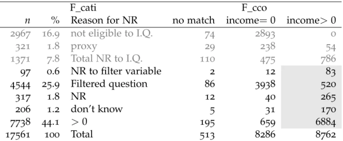
Table 1.1 – Detailed nonresponse affecting employee personal income, CATI-variable. (NR = nonresponse, I.Q. = individual questionnaire, F_cati = nonresponse flag for vari-able yCATI). Nonresponse affecting the corresponding register variable (due to the failure of matching) is also detailed (F_cco = nonresponse flag for variable ycco).

F_cati F_cco

n % Reason for NR no match income=0 income>0 2967 16.9 not eligible to I.Q. 74 2893 0

321 1.8 proxy 29 238 54 1371 7.8 Total NR to I.Q. 110 475 786 97 0.6 NR to filter variable 2 12 83 4544 25.9 Filtered question 86 3938 520 317 1.8 NR 12 40 265 206 1.2 don’t know 5 31 170 7738 44.1 >0 195 659 6884 17561 100 Total 513 8286 8762

We decided to restrict the study to the cases highlighted by the shaded area of Table 1.1. These correspond to observations with a strictly positive value to the CCO-variable and where, simultaneously, the CATI-variable showed item nonresponse (the categories corresponding to the first three rows of the Table have been excluded since they correspond to total nonre-sponse, which is treated by reweighting). Individuals of interest are those whose CCO-income is reported in Table 1.2.

Our framework is the following: we aim to develop an imputation method for the variable yCATI = P09I57G_cati which is subject to an

un-1

The CCO is based in Geneva, it is a public institution active in the field of social insurance 1st_{(AVS / AI / APG), http://www.zas.admin.ch/cdc/.}

known nonresponse mechanism. Luckily, we also have the complete vari-able yCCO = P09I57G_cdc. We apply the nonresponse observed for yCATI

to yCCO and develop the imputation method for yCCO. As we know the

true values of yCCO, we can evaluate the performance of the method.

By observing Table 1.2, we immediately notice that the nature of non-response to yCATI is dependent on the level of income of the person. It is

clearly a case of nonignorable nonresponse (NMAR) (Non Missing At

Ran-dom, in the sense of Little & Rubin, 2002), see Chapter 5 for more details).

Table 1.2 – Descriptives statistics of employee’s income, CCO-variable, depending on the reasons for nonresponse to CATI.

n % F_cati Mean Median SD Min Max

83 1.0 NR to filter variable 12’165 8’126 13’462 278 69’502 520 6.6 Filtered question 23’580 9’214 47’760 16 511’775 265 3.3 NR 79’050 69’200 74’406 322 559’013 170 2.1 don’t know 59’729 31’239 116’090 320 1’132’000 6884 86.9 >0 70’250 61’936 63’718 100 1’758’845 7922 100.0

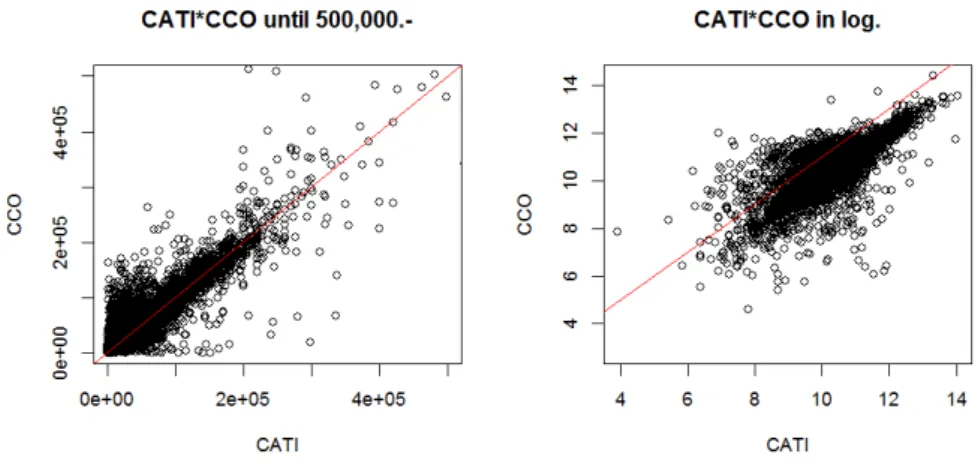
Note that variables yCATI and yCCO do not behave in quite the same

way. Indeed, the information collected by the telephone survey is not systematically very close to the one in the register. However, the two vari-ables correlate to 84%. Figure 1.1 gives a graphical view of the relationship between the two variables.

Figure 1.1 – Employee’s income collected by CATI versus CCO-register value.

As will be recalled in Chapters 3 and 5, we further restricted the num-ber of observations regarding the imputation model on units for which two other continuous variables were available, namely the housing costs and the occupation rate for the surveyed individuals. The number of full cases amounts to 6,188 out of 7,922 individuals, which means 21.89% non-response.

2

Sondage dans des registres

de population et de ménages

en

Suisse : coordination

d

’enquêtes, pondération et

imputation

Abstract

L’Office Fédéral de la Statistique harmonise ses enquêtes par échantillonnage auprès des personnes et des ménages en Suisse. Dans cet article, nous présen-tons un aperçu des méthodes actuellement utilisées. Les échantillons sont sélec-tionnés de manière coordonnée afin de répartir au mieux la charge d’enquête sur les ménages et les personnes. Le calcul des pondérations, dont on présente les principales étapes, est adapté aux différents besoins et aux différentes situa-tions rencontrées. L’Office se base sur les recommandasitua-tions internationales, dont il participe à l’élaboration, pour le traitement des données d’enquête et les im-putations. La précision des estimateurs est systématiquement évaluée en tenant compte des traitements réalisés. 1

The Swiss Federal Statistical Office is currently harmonizing its population and household survey operations. In this paper, we give an overview of its pro-duction methods. Samples are selected with coordination so as to spread the survey burden over the population. The computation of extrapolation weights adapted to different cases and needs is presented with its main steps. The Of-fice relies on international recommendations for data editing and imputation, and contributes to their elaboration. The precision of estimators is consistently evaluated, according to the different treatments and methods involved in their construction.

Keywords: calage, variance, segmentation, valeurs aberrantes, census, calibration, variance, segmentation, outliers

1

This chapter is a an authorized reprint of: Graf, E. & Qualité, L. (2014). Sondage dans des registres de population et de ménages en Suisse : coordination d’enquêtes, pondéra-tion et imputapondéra-tion. Journal de la Société Française de Statistique 155 No.4, 95–133.

2

.1

Introduction

L’Office Fédéral de la Statistique (OFS) achève d’harmoniser ses enquêtes par échantillonnage auprès des personnes et des ménages en Suisse. Dans cet article, nous présentons un aperçu des méthodes actuellement util-isées par l’office. Il ne s’agit en aucun cas d’un manuel de bonnes pratiques, mais de l’exposé de solutions et compromis qui ont été réal-isés pour les besoins spécifiques de l’OFS. L’uniformisation des méth-odes d’échantillonnage, de pondération, et de traitement des données d’enquête est l’occasion de réévaluer toutes ces pratiques pour en dégager un corpus de méthodes solide et applicable aux divers cas rencontrés par l’office.

Dans une première partie, nous décrivons les enquêtes auprès de la population et auprès des ménages réalisées par l’OFS. On y présente les pendants suisses de grandes enquêtes européennes ainsi que le nouveau système de recensement, en partie basé sur des enquêtes annuelles par échantillonnage, qui remplace le recensement décennal de la population.

Dans une deuxième partie, nous présentons la méthode de tirage avec coordination utilisée pour les enquêtes du nouveau système de re-censement et qui sera utilisée à terme pour toutes les enquêtes de l’OFS. Le tirage coordonné d’échantillons permet de mieux répartir la charge d’enquête sur la population.

Dans la troisième partie, nous présentons les méthodes d’estimation et de pondération utilisées pour les enquêtes de l’OFS. Les estimateurs utilisés sont en principe des estimateurs par dilatation, c’est-à-dire des sommes pondérées de valeurs observées (ou imputées). Nous présentons les étapes-clés de la construction des pondérations : calcul des probabil-ités d’inclusion dans l’échantillon, estimation des probabilprobabil-ités de réponse, partage des poids, combinaison d’échantillons, calages.

Dans la quatrième partie, nous présentons le principe de traitement des données et d’imputation appliqué à l’OFS. L’Office suit les recomman-dations issues de plusieurs grands projets européens quant au traitement des valeurs manquantes, aberrantes, erronées ou extrêmes. Nous men-tionnons les principales techniques d’imputation utilisées en production.

Dans la cinquième partie, nous traitons les méthodes d’estimation de la variance utilisées à l’OFS. Celles-ci sont pensées pour tenir le mieux possible compte des principaux facteurs influençant la variance des esti-mateurs produits : le plan de sondage, la non-réponse et son traitement, les partages ou combinaisons de poids, enfin les calages et imputations. Dans la pratique, un compromis doit être réalisé car la prise en compte de tous ces aspects rend le problème extrêmement complexe. Des approxi-mations simples sont donc utilisées.

Dans la sixième partie, nous donnons un aperçu sur les évolutions planifiées dans un futur proche : le traitement de la non-réponse par calage généralisé, l’estimation de la variance due à l’imputation ainsi que les dernières améliorations prévues quant à la coordination des échantil-lons.

2.2. Les différentes enquêtes auprès de la population des personnes et des ménages résidant

en Suisse 33

2

.2

Les différentes enquêtes auprès de la population

des personnes et des ménages résidant en

Suisse

2.2.1 Le nouveau système de recensement de la population suisse

Le traditionnel recensement décennal de la population suisse est rem-placé, depuis 2010, par la création et l’exploitation par l’OFS d’un cadre d’échantillonnage2

de population et de ménages appelé SRPH (Stich-probenrahmen für Personen und Haushaltserhebungen), et un système d’enquêtes annuelles. L’office ne gère pas de registre centralisé de la pop-ulation, mais utilise différents registres pour créer le fichier SRPH. Celui-ci est essentiellement construit en agrégeant les registres administratifs du contrôle des habitants des communes et des cantons. L’inscription dans le registre de la commune de résidence est en effet obligatoire en Suisse, à quelques exceptions près, parmi lesquelles on peut citer les personnes ayant le statut de fonctionnaire international. Le fichier ainsi obtenu est encore enrichi par l’utilisation de registres fédéraux : le registre des de-mandeurs d’asile, le registre central des étrangers, le registre des fonc-tionnaires internationaux et le registre informatisé de l’état civil Infostar. La livraison des données par les communes et cantons, et la création du cadre d’échantillonnage, sont effectuées quatre fois par an, en dates de valeur des 31 décembre, 31 mars, 30 juin et 30 septembre. Les données sont disponibles environ six semaines après ces dates de référence.

Le fichier SRPH contient des informations démographiques basiques sur les personnes habitant en Suisse : sexe, date de naissance, état civil, permis de séjour, nationalité, date d’arrivée en Suisse et au lieu de rési-dence actuel, ainsi que l’adresse, le statut de résirési-dence (résirési-dence princi-pale dans un ménage privé, résidence secondaire, ménage collectif, etc.). L’OFS a la conviction que ce répertoire offre une très bonne couverture de la population résidant de manière permanente en Suisse, l’inscription au registre de la commune étant nécessaire pour bénéficier d’un certain nombre de prestations, et déterminante pour le recouvrement de l’impôt sur le revenu. La pertinence de ce cadre de sondage pour les opérations statistiques est garantie par l’utilisation permanente du numéro unique de sécurité sociale comme identifiant à toutes les étapes de sa création, ainsi que par des procédures de contrôle de la qualité, depuis la livraison des données par les communes jusqu’à la constitution finale du fichier SRPH. Depuis la fin décembre 2012, les communes ont l’obligation légale de fournir le numéro de bâtiment et de logement de chaque personne. Ces numéros, qui permettent de connaître la constitution des ménages, sont extraits du registre des bâtiments et logements entretenu à l’OFS. Cette obligation était déjà largement respectée depuis 2010, mais avec une cer-taine hétérogénéité selon les cantons et communes.

Le premier élément du nouveau système de recensement est le résultat de l’exploitation, chaque année, du répertoire de population du 31 décem-bre précédent. Les données utilisées pour constituer le fichier SRPH du

2

La locution “cadre d’échantillonnage” utilisée en Suisse est équivalente à “base de sondage”. Il s’agit de la traduction du mot allemand “Stichprobenrahmen”.

31décembre font l’objet de traitements supplémentaires pour produire la statistique de la population et des ménages (Statpop). Cette exploitation permet de fournir une première série de résultats, et également la pop-ulation de référence pour les enquêtes complémentaires du système de recensement. Les données démographiques individuelles sont utilisées. Le taux de couverture de cette statistique sera évaluée sur la base d’une enquête réalisée en 2013. La constitution des ménages n’a pas été exploitée pour ces premiers résultats de comptages, tant que l’obligation légale de renseigner n’était pas en vigueur. Elle est par contre utilisée dans les pro-cessus de production de l’OFS au moment de l’échantillonnage.

Le deuxième élément du nouveau système de recensement est une enquête annuelle, par échantillonnage aléatoire, de grande ampleur : l’enquête structurelle. L’échantillon de base, financé par la confédéra-tion helvétique, est dimensionné de manière à obtenir approximativement 200’000 questionnaires renseignés par des personnes ayant leur résidence permanente en Suisse, et âgées de 15 ans ou plus. Cela représente un taux de sondage de 3% environ. Les cantons et communes peuvent fi-nancer une augmentation de l’échantillon les concernant, jusqu’à le dou-bler. Ponctuellement, en 2010, ils avaient la possibilité de quadrupler l’échantillon. Le questionnaire de cette enquête reprend en grande par-tie les questionnaires des recensements précédents en omettant les infor-mations disponibles dans le cadre d’échantillonnage SRPH. Les thèmes abordés sont, entre autres, le niveau d’éducation, le statut d’activité et la branche d’activité, les trajets domicile-travail, la langue employée, la composition du ménage et les relations familiales, ainsi que le statut d’occupation du logement et le loyer s’il y a lieu. Le taux de réponse ob-servé à cette enquête obligatoire est de 90% environ. Le mode de collecte est en principe le questionnaire papier à retourner ou la télédéclaration par internet, le choix étant laissé au répondant.

Le troisième élément du système de recensement suisse est une en-quête thématique annuelle, avec un échantillon de base de 10’000 à 40’000 répondants selon le thème. Chacun des cinq thèmes suivants est traité à son tour tous les cinq ans : la mobilité et les transports, la formation initiale et continue, la santé, la famille, les langues les religions et les cultures. L’échantillon de ces enquêtes est constitué de 3 à 4 blocs sélec-tionnés dans les différents cadres d’échantillonnage de l’année d’enquête. La collecte est principalement réalisée par entretien téléphonique assisté par ordinateur. Enfin, le quatrième élément du système de recensement est une enquête téléphonique annuelle auprès d’environ 3’000 répondants, appelée enquête Omnibus, sur des thèmes qui sont décidés chaque année. Tous ces échantillons sont sélectionnés dans le cadre d’échantillonnage le plus récent. L’OFS fournit également des échantillons tirés dans le SRPH pour les enquêtes menées par d’autres institutions sur des thèmes d’intérêt national, dont en particulier les projets soutenus par le Fonds National de la Recherche Scientifique.

L’apparition de l’enquête structurelle, qui touche chaque année une part non négligeable de la population suisse, a motivé l’utilisation d’une procédure pour coordonner les échantillons de l’OFS. En effet, si l’on ne

2.2. Les différentes enquêtes auprès de la population des personnes et des ménages résidant

en Suisse 35

prenait aucune mesure pour l’éviter, des dizaines de milliers de person-nes seraient sélectionnées à deux enquêtes structurelles successives ou à plusieurs enquêtes de l’OFS en même temps, sans que cela n’ait une util-ité statistique. Cela pourrait conduire à une baisse des taux de réponse, à une dégradation de l’image de l’office et à une surcharge de travail liée au traitement des plaintes venant du public. On essaye donc d’éviter de sol-liciter de manière répétée les personnes et les ménages lorsque cela n’est pas utile. La procédure de sélection coordonnée d’échantillons utilisée à l’OFS pour répondre à ce besoin est décrite en Section 2.3.

2.2.2 Les enquêtes sur les conditions de vie, le budget des ménages et

la population active

Outre les enquêtes du système de recensement, l’OFS réalise chaque année trois grandes enquêtes par échantillonnage auprès des ménages et des personnes résidant de manière permanente en Suisse dans des ménages privés. Il s’agit de l’enquête sur les revenus et conditions de vie SILC (Survey on Income and Living Conditions), l’Enquête sur le Budget des Ménages (EBM), et l’Enquête Suisse sur la Population Active (Espa).

L’enquête SILC est la source de référence pour les comparaisons statis-tiques en matière de distribution de revenu et d’exclusion sociale pour l’Union Européenne. Elle est, depuis 2007, le pendant suisse de l’enquête européenne EU-SILC réalisée dans plus de 30 pays d’Europe. Elle doit de ce fait satisfaire aux exigences et recommandations données par Euro-stat dans de nombreux domaines, en particulier sur la manière de calculer les pondérations (Eurostat, 2004b, 2005b; Graf, 2008a), sur les tailles mini-males des échantillons de répondants, ménages et individus (Graf, 2006), et enfin sur la précision des indicateurs clés qui sont livrés chaque année à Eurostat.

L’enquête SILC utilise un panel rotatif de répondants : chaque an-née, un quart de l’échantillon est renouvelé, et chaque ménage enquêté est théoriquement sollicité pendant quatre années. Elle permet ainsi de produire des résultats pour une année donnée, mais aussi d’estimer des évolutions avec une bonne précision. SILC est réalisée annuellement par téléphone auprès d’environ 7’000 ménages comprenant 17’000 personnes. L’objectif principal de l’enquête Espa est de fournir des données sur la structure de la population active et sur les comportements en matière d’activité professionnelle. Grâce à l’application stricte de définitions inter-nationales, les données de la Suisse peuvent être comparées avec celles des pays de l’OCDE et de l’Union européenne. Il s’agit d’une enquête auprès des personnes, qui est réalisée chaque année depuis 1991. L’organisation de l’enquête a été revue en 2010 pour permettre d’obtenir des estimations trimestrielles, mais aussi des estimations d’évolutions trimestrielles et an-nuelles précises. Les unités enquêtées sont ré-interrogées après 3, 12 et 15 mois, avant de sortir de l’échantillon. À un trimestre donné, l’échantillon est constitué de quatre blocs. L’un est interrogé pour la première fois, et les autres respectivement pour la deuxième, troisième et quatrième fois (Renfer, 2009; OFS, 2012). L’échantillon de l’Espa est complété par un

échantillon de personnes de nationalité étrangère sélectionné dans le reg-istre central des étrangers (Système d’information central sur la migration - Symic). L’Espa est réalisée auprès d’un échantillon annuel d’environ 105’000 personnes, augmenté d’un sur-échantillon annuel de 21’000 per-sonnes étrangères.

Les résultats de l’EBM permettent d’adapter chaque année la compo-sition du panier-type pour le calcul de l’indice suisse des prix à la con-sommation, ainsi que d’étudier la structure et l’évolution des revenus et des dépenses des ménages. Cette enquête se base sur des fondements et définitions méthodologiques en accord avec les directives internationales, notamment la nomenclature des fonctions de consommation des ménages COICOP (Classification Of Individual COnsumption by Purpose) définie par le Bureau International du Travail (BIT). L’EBM comporte environ 3’000 ménages interviewés chaque année. L’échantillon de l’EBM est par-titionné en douze sous-échantillons qui sont interrogés chacun leur tour durant un mois. Cette enquête est réalisée annuellement à l’OFS depuis 2000.

Hormis l’échantillon spécifique d’étrangers de l’Espa, les échantillons de ces trois enquêtes sont tous actuellement sélectionnés dans le reg-istre de numéros de téléphone Castem (Cadre de sondage pour le tirage d’échantillons de ménages) constitué à partir des livraisons des opéra-teurs téléphoniques actifs en Suisse. La collecte de données est en principe réalisée par entretien téléphonique assisté par ordinateur, éventuellement complétée par des questionnaires papiers ou électroniques. Afin de limiter la charge d’enquête demandée à la population, les numéros de téléphone qui ont été sélectionnés pour une enquête sont écartés pour une durée déterminée de la liste des numéros sélectionnables. Cette pratique est, à l’OFS, appelée “historisation”. Cette procédure n’est acceptable sur le plan méthodologique que lorsque les échantillons représentent une part négligeable et non spécifique de la population. D’ici à la fin 2014, les échantillons de ces trois enquêtes seront désormais sélectionnés dans le cadre d’échantillonnage SRPH. Elles pourront ainsi être coordonnées avec les enquêtes du système de recensement. La procédure “d’historisation” des numéros de téléphone déjà sélectionnés sera abandonnée au profit de la méthode de coordination développée pour le système de recensement.

2

.3

Enquêtes coordonnées dans le fichier SRPH

La méthode décrite dans cette section permet la sélection d’échantillons positivement ou négativement coordonnés, c’est à dire d’échantillons dont l’intersection est volontairement importante ou au contraire petite, voire vide. Une coordination négative est utile pour répartir la charge d’enquête équitablement sur la population en évitant que les mêmes unités soient sélectionnées dans plusieurs échantillons lorsque cela n’est pas néces-saire. Elle devient particulièrement importante lorsqu’un grand nombre d’enquêtes sont réalisées, dont certaines ont de forts taux de sondage. Une coordination positive est souhaitable lorsque l’on veut mettre à jour un échantillon de panel, ou lorsque l’on veut pouvoir comparer avec précision

2.3. Enquêtes coordonnées dans le fichier SRPH 37

les résultats d’une nouvelle enquête avec ceux d’une enquête précédente. La méthode proposée est utilisable avec des probabilités d’inclusion iné-gales, dans une population dynamique avec des naissances, ou entrées, et des décès, ou sorties, d’unités.

La coordination des échantillons est un problème qui a et qui continue d’être largement étudié, et pour lequel de nombreuses solutions ont été développées en particulier par les Instituts Nationaux de Statistique (INS). On peut entre autres se référer à Patterson (1950); Keyfitz (1951); Kish & Scott (1971); Rosén (1997a,b); Brewer et al. (1972); De Ree (1983); Van Huis et al. (1994a,b); Cotton & Hesse (1992a,b); Rivière (1998, 1999, 2001a,b); Ohlsson (1995); Ernst (1996) et Kröger et al. (1999). Les méthodes de co-ordination développées dans les INS sont essentiellement prévues pour fonctionner avec des plans de sondage aléatoires simples ou stratifiés. Il est toutefois apparu très difficile de développer une méthode de tirage co-ordonnée qui respecte exactement ces plans de sondage lorsque la popula-tion et la définipopula-tion des strates changent entre les enquêtes. A l’exceppopula-tion de l’enquête Espa qui contient un sur-échantillon d’étrangers, les plans de sondage pour les enquêtes de l’OFS ont tous des spécifications très sem-blables : les probabilités d’inclusion sont uniformes au sein des cantons ou des communes pour toutes les personnes résidentes permanentes âgées de 15 ans ou plus. Cependant, les échantillons que l’OFS fournit à ses parte-naires pour leurs propres enquêtes peuvent avoir des caractéristiques très diverses. Ces instituts peuvent par exemple souhaiter cibler des sous-populations spécifiques identifiables grâce aux données contenues dans le SRPH. Il a donc été nécessaire de développer un système très souple qui permette de se départir d’une stratification fixe.

Brewer et al. (1972) ont inventé l’approche dite des numéros aléatoires permanents. Ce sont des méthodes qui reposent sur l’utilisation d’un même jeu de nombres aléatoires pour sélectionner les différents échantil-lons au cours du temps. Dans certains cas, dont celui qui est présenté ici, un nombre aléatoire entre 0 et 1 est attribué à chaque unité lorsqu’elle entre dans la population ou dans le cadre de sondage, et ce nombre lui reste attaché jusqu’à ce qu’elle sorte de la population ou du cadre. D’autres méthodes nécessitent de permuter les nombres aléatoires entre unités de la population, suivant les tirages passés (Cotton & Hesse, 1992a; Rivière, 2001a). Une des caractéristiques de la méthode de Brewer et coll. Brewer et al. (1972) est qu’elle permet de choisir librement les probabil-ités d’inclusion de chaque unité de la population à chaque enquête. Elle ne requiert donc pas de stratification fixe de la population et possède la flexibilité nécessaire à l’OFS. Une présentation des méthodes à nombres aléatoires permanent se trouve dans Ohlsson (1995).

2.3.1 Coordination d’échantillons

Il existe différentes définitions de ce qu’est la coordination d’échantillons. Le fait que les processus aléatoires qui permettent de sélectionner les échantillons de deux enquêtes soient ou non indépendants n’est pas ce qui est réellement intéressant. Une définition utile conduit à minimiser

ou bien à maximiser, et généralement à contrôler le nombre d’unités com-munes à deux échantillons. La notion que nous utilisons ici est légèrement différente, et plus adaptée au cas des enquêtes à probabilités inégales : nous travaillons sur les probabilités, pour chaque unité, d’appartenir si-multanément à deux ou une certaine collection d’enquêtes. Considérons un plan de sondage pour T enquêtes, c’est à dire une loi de probabilité

P(s1, s2, . . . , sT),

sur les T échantillons sélectionnables s1, s2, . . . , sT. Ces échantillons ne sont pas nécessairement tous sélectionnés dans la même population. Les distri-butions marginales d’ordre 1 de P(·)sont les plans de sondages (appelés transversaux) des T enquêtes considérées. La probabilité qu’une unité k soit sélectionnée dans un échantillon si est désignée par

πi

k =P(si ∋ k),

et la probabilité qu’une unité k soit sélectionnée dans l’échantillon si et dans l’échantillon sj est notée

πi,j

k =P(si ∋k & sj ∋ k).

Definition 2.1 On dit qu’il y a une coordination positive pour l’unité k entre les enquêtes i et j

si πi,j k > π i k·π j k, et qu’il y a une coordination négative si au contraire

πi,j k < π i k·π j k.

La coordination, positive ou négative, est dite optimale pour l’unité k si le max-imum ou minmax-imum théorique de πi,j_k , qui vaut respectivement min(π_ki,π_kj) et

max(0,π_ki +π_kj −1), est atteint.

Si la coordination est optimale et positive (resp. négative) entre les enquêtes i et j, au sens de la définition 2.1, pour toutes les unités, alors la taille espérée de l’intersection des échantillons si _{et s}j_,

ni,j =E [ #(si∩sj) ] =

∑

k πi,j k ,

est maximale (resp. minimale). Cela signifie que parmi toutes les dis-tributions de probabilité P(·) sur les couples d’échantillons, ayant des marginales fixées P(si_{) et P(s}j_{), la valeur de n}i,j _{est maximale (resp.}

minimale) lorsque P(·) fournit une coordination positive optimale (resp. négative optimale) pour toutes les unités k selon la définition 2.1. Cela n’implique pas que la taille #(si_∩sj_{)de l’intersection des échantillons s}i