HAL Id: hal-02951111
https://hal.archives-ouvertes.fr/hal-02951111
Submitted on 8 Oct 2020
HAL is a multi-disciplinary open access
archive for the deposit and dissemination of
sci-entific research documents, whether they are
pub-lished or not. The documents may come from
teaching and research institutions in France or
abroad, or from public or private research centers.
L’archive ouverte pluridisciplinaire HAL, est
destinée au dépôt et à la diffusion de documents
scientifiques de niveau recherche, publiés ou non,
émanant des établissements d’enseignement et de
recherche français ou étrangers, des laboratoires
publics ou privés.
global models
Maarten Krol, Marco de Bruine, Lars Killaars, Huug Ouwersloot, Andrea
Pozzer, Yi Yin, Frederic Chevallier, Philippe Bousquet, Prabir Patra, Dmitry
Belikov, et al.
To cite this version:
Maarten Krol, Marco de Bruine, Lars Killaars, Huug Ouwersloot, Andrea Pozzer, et al.. Age of air as
a diagnostic for transport timescales in global models. Geoscientific Model Development, European
Geosciences Union, 2018, 11 (8), pp.3109-3130. �10.5194/GMD-11-3109-2018�. �hal-02951111�
https://doi.org/10.5194/gmd-11-3109-2018 © Author(s) 2018. This work is distributed under the Creative Commons Attribution 4.0 License.
Age of air as a diagnostic for transport timescales in global models
Maarten Krol1,2,3, Marco de Bruine2, Lars Killaars4, Huug Ouwersloot5, Andrea Pozzer5, Yi Yin6,a,Frederic Chevallier6, Philippe Bousquet6, Prabir Patra7, Dmitry Belikov8, Shamil Maksyutov9, Sandip Dhomse10, Wuhu Feng11, and Martyn P. Chipperfield10,11
1Meteorology and Air Quality, Wageningen University, Wageningen, the Netherlands 2Institute for Marine and Atmospheric Research, Utrecht University, Utrecht, the Netherlands 3Netherlands Institute for Space Research SRON, Utrecht, the Netherlands
4Faculty of Science and Engineering, University of Groningen, Groningen, the Netherlands 5Max Planck Institute for Chemistry, Mainz, Germany
6Laboraroire de Sciences du Climat et de l’Environnement (LSCE), Gif-sur-Yvette, France 7Japan Agency for Marine-Earth Science and Technology (JAMSTEC), Yokohama City, Japan 8Hokkaido University, Sapporo, Hokkaido, Japan
9Center for Global Environmental Research, National Institute for Environmental Studies, Tsukuba, Ibaraki, Japan 10School of Earth and Environment, University of Leeds, Leeds, UK
11National Centre for Atmospheric Science, University of Leeds, Leeds, UK anow at: Jet Propulsion Laboratory, Pasadena, California, USA
Correspondence: Maarten Krol ([email protected])
Received: 18 October 2017 – Discussion started: 7 November 2017
Revised: 16 July 2018 – Accepted: 19 July 2018 – Published: 3 August 2018
Abstract. This paper presents the first results of an age-of-air (AoA) inter-comparison of six global transport models. Following a protocol, three global circulation models and three chemistry transport models simulated five tracers with boundary conditions that grow linearly in time. This allows for an evaluation of the AoA and transport times associated with inter-hemispheric transport, vertical mixing in the tro-posphere, transport to and in the stratosphere, and transport of air masses between land and ocean. Since AoA is not a directly measurable quantity in the atmosphere, simula-tions of222Rn and SF6 were also performed. We focus this
first analysis on averages over the period 2000–2010, taken from longer simulations covering the period 1988–2014. We find that two models, NIES and TOMCAT, show substan-tially slower vertical mixing in the troposphere compared to other models (LMDZ, TM5, EMAC, and ACTM). However, while the TOMCAT model, as used here, has slow transport between the hemispheres and between the atmosphere over land and ocean, the NIES model shows efficient horizontal mixing and a smaller latitudinal gradient in SF6compared to
the other models and observations. We find consistent differ-ences between models concerning vertical mixing of the
tro-posphere, expressed as AoA differences and modelled222Rn gradients between 950 and 500 hPa. All models agree, how-ever, on an interesting asymmetry in inter-hemispheric mix-ing, with faster transport from the Northern Hemisphere sur-face to the Southern Hemisphere than vice versa. This is attributed to a rectifier effect caused by a stronger seasonal cycle in boundary layer venting over Northern Hemispheric land masses, and possibly to a related asymmetric position of the intertropical convergence zone. The calculated AoA in the mid–upper stratosphere varies considerably among the models (4–7 years). Finally, we find that the inter-model dif-ferences are generally larger than difdif-ferences in AoA that re-sult from using the same model with a different resolution or convective parameterisation. Taken together, the AoA model inter-comparison provides a useful addition to traditional ap-proaches to evaluate transport timescales. Results highlight that inter-model differences associated with resolved trans-port (advection, reanalysis data, nudging) and parameterised transport (convection, boundary layer mixing) are still large and require further analysis. For this purpose, all model out-put and analysis software are available.
1 Introduction
The composition of the atmosphere is determined by ex-change processes at the Earth’s surface, transport processes within the atmosphere, and chemical and physical conver-sion processes. For example, the atmospheric distribution of the CH4mixing ratio is driven by natural and anthropogenic
emissions at the Earth’s surface, atmospheric transport, and removal that is primarily driven by the atmospheric oxidants OH, Cl, and O(1D) (Myhre et al., 2013). The estimated at-mospheric lifetime of CH4is approximately 9 years (Prather
et al., 2012) mainly due to oxidation within the troposphere. Although some CH4 destruction occurs in the stratosphere
(Boucher et al., 2009), as witnessed by the decaying mixing ratios with altitude, the slow atmospheric transport from the troposphere to the stratosphere limits its impact on the at-mospheric lifetime of CH4. Other atmospheric constituents
have widely different budgets. SF6, for instance, has purely
anthropogenic sources, mostly in the Northern Hemisphere (NH), and is only broken down in the upper stratosphere (Kovács et al., 2017), resulting in a very long atmospheric lifetime of more than 1000 years. In contrast,222Rn emanates naturally from land surfaces and quickly decays radioactively with a half-life of 3.8 days.
To better understand the changes in the atmosphere, gen-eral circulation models (GCMs) or chemistry transport mod-els (CTMs) are used to simulate its composition. While CTMs use archived meteorological fields to calculate trans-port, GCMs calculate their own meteorology. To track the ob-served state of the atmosphere, the GCMs can be nudged to-wards meteorological reanalysis data (e.g. Law et al., 2008). Comparing results of these models to atmospheric obser-vations allows the assessment of the model performance. Depending on the atmospheric compound, various aspects of atmospheric transport can be investigated. Jacob et al. (1997) used 222Rn and other short-lived tracers to evaluate the convective and synoptic-scale transport in CTMs. Since the early 1990s, the atmospheric tracer transport model inter-comparison project (TransCom) has carried out studies to quantify and diagnose the uncertainty in inversion calcula-tions of the global carbon budget that result from errors in simulated atmospheric transport. Initially, TransCom focused on non-reactive tropospheric species such as SF6(Denning
et al., 1999) and CO2(Law et al., 1996, 2008). A more
re-cent TransCom model inter-comparison (Patra et al., 2011) focused on the ability of models to properly represent at-mospheric transport of CH4, focussing on vertical gradients,
its average long-term trends, seasonal cycles, inter-annual variations (IAVs) and inter-hemispheric (IH) gradients. The study concluded that models with faster IH exchange for SF6have smaller IH gradients in CH4. The estimated IH
ex-change time, calculated based on a time-invariant SF6
emis-sion rate, remained relatively constant over the period of the analysis (1996–2007). Interestingly, a recent study high-lighted the importance of IH transport variations in
explain-ing the CO2mixing ratio difference between Mauna Loa in
the NH and Cape Grim, Tasmania, in the Southern Hemi-sphere (SH) (Francey and Frederiksen, 2016). Specifically, the 0.8 ppm step-like increase in this difference between 2009 and 2010 was attributed to the opening and closing of the upper-tropospheric equatorial westerly duct (Waugh and Funatsu, 2003), with an open-duct pattern from July 2008 to June 2009 (fast IH exchange), followed by closed-duct conditions from July 2009 to June 2010 (slow IH exchange). Confirming this mechanism, Pandey et al. (2017) also found faster IH transport of CH4during the strong La Niña in 2011
using the TM5 CTM. The timescale of IH transport is an im-portant parameter for atmospheric inversion studies. In these studies atmospheric observations are used to infer surface flux magnitude and distribution. For a long-lived greenhouse gas like CH4fast IH transport implies that a larger fraction of
the emissions will be attributed to the NH (Patra et al., 2014, 2011).
The efficiency of models to mix the planetary boundary and to vent emissions to the overlying free atmosphere has been studied using SF6and has generally revealed too slow a
mixing over midlatitude continents in the TM5 (Peters et al., 2004) and MOZART models (Gloor et al., 2007). Together with the convective parameterisation, this determines the rate by which emissions (e.g. SF6and222Rn) are mixed vertically
and inter-hemispherically (Locatelli et al., 2015a).
Another transport timescale relevant for atmospheric composition studies is troposphere–stratosphere exchange (Holton et al., 1995), driven by the Brewer–Dobson circu-lation (Butchart, 2014). Depending on the greenhouse gas scenario, global climate model projections predict an accel-eration of this global mass circulation of tropospheric air through the stratosphere. Stratospheric AoA and its temporal trend have been determined from SF6 measurements from
the MIPAS satellite (Stiller et al., 2012) and from balloon observations (Engel et al., 2009). Using a suite of strato-spheric observations, Fu et al. (2015) quantified the acceler-ation of the Brewer–Dobson circulacceler-ation as 2.1 % per decade for 1980–2009. Other modelling and experimental studies re-vealed that the atmospheric composition of the tropopause layer strongly depends on the mixing processes that occur on a wide range of spatiotemporal scales (Berthet et al., 2007; Hoor et al., 2010; Prather et al., 2011; Hsu and Prather, 2014).
Transport of trace gases in CTMs and GCMs is deter-mined by several factors, for which various choices are pos-sible. First, winds and the choice of advection scheme drive the large-scale dispersion and IH transport of tracers. While CTMs directly use winds from a meteorological reanalysis product, GCMs calculate their own meteorology and option-ally apply a nudging scheme to simulate the transport of trac-ers (e.g. Law et al., 2008). Second, parameterised sub-grid-scale processes such as boundary layer mixing and convec-tion determine vertical gradients and the rate of IH transport (e.g. Locatelli et al., 2015a). Finally, other differences may be
caused by the horizontal and vertical grid of the model and other issues related to spatial and temporal integration. For example, by doubling the vertical resolution of their GCM, Locatelli et al. (2015a) largely improved the representation of SF6transport from the troposphere to the stratosphere.
Sim-ilarly, Bând˘a et al. (2015) reported large differences in the stratospheric dispersion of the 1991 Pinatubo plume when increasing the vertical resolution in TM5 from 34 to 60 lev-els.
To investigate the impact of these choices on the partic-ipating models, this paper will present the first results of the TransCom AoA inter-comparison study. The concept of AoA originates from stratospheric studies (Hall and Prather, 1993; Hall and Plumb, 1994; Neu and Plumb, 1999; Hall et al., 1999). In brief, the age spectrum in the stratosphere G(x, t |t0) is calculated as a type of Green’s function that
propagates a tropospheric mixing ratio boundary condition into the stratosphere. Given a location x in the stratosphere, Gδt represents the fraction of air at x that was lost in the tro-posphere in the time interval between t − t0and t − t0+δt
(Hall et al., 1999). In practical model applications focussing on stratospheric age spectra, G(x, t |t0)is calculated as the
response of a time-dependent boundary condition δ(t − t0)
specified in a forcing volume in the troposphere. More re-cently, this concept has also been applied to tropospheric studies (Holzer and Hall, 2000; Waugh et al., 2013; Holzer and Waugh, 2015). In this AoA inter-comparison, we will only analyse the mean AoA. In the terminology of Holzer and Hall (2000), AoA is defined as the mean transit time, with the age spectrum being the transit-time probability den-sity function. This property can be easily extracted from model simulations of a passive tracer with linearly grow-ing boundary conditions in a specified atmospheric volume. We will outline the inter-comparison protocol in Sect. 2. The resulting model output focussing on the simulation period 2000–2010 is compared in Sect. 3 and discussed in Sect. 4. Finally, the main conclusions are summarised in Sect. 5.
2 Method
2.1 AoA protocol
In order to compare transport timescales of a suite of CTMs and GCMs, a protocol was developed that allows a straight-forward implementation in existing atmospheric models. We defined five AoA tracers (Table 1) for which linearly grow-ing boundary conditions are applied. These AoA tracers are chosen to study IH transport, transport to the stratosphere, and air mass transport between land and ocean. The mixing ratios of these tracers in the models are initialised to zero on 1 January 1988 and simulations are run to the end of 2014.
According to the protocol, the mixing ratio of each AoA tracer in its respective forcing volume is set every time step to a value B = f × t , with t the elapsed time (in
Table 1. The five AoA tracers and their forcing volume. AoA tracer Forcing volume
Surface Surface < 100 m NHsurface NH surface < 100 m SHsurface SH surface < 100 m Land Land < 100 m Ocean Ocean < 100 m
s) since January 1988 and f a forcing constant of 1 × 10⁻¹⁵mol mol−1s−1. As a result, the mixing ratio in the forcing volume will have a value of 852.0768 nmol mol−1 at the end of the simulation and lower values elsewhere. In theory, numerical issues with advection might lead to small wiggles in the vicinity of strong mixing ratio gradients. This may result in small unphysical negative mixing ratios that cannot be handled by some model transport schemes. To remedy this, models may be initialised with a uniform 100 nmol mol−1 initial condition, a value that is subtracted before further analysis.
Modellers are requested to calculate the exact fraction of each grid box within the forcing volume. This calculation in-volves the land mask, the fraction of the grid box in either the NH and SH, and the geopotential height. The protocol pro-vides example code to help with the implementation. Impor-tantly, the mixing ratio of the grid boxes within the forcing volume was set according to
Xnew=fset×B + (1 − fset) × Xold, (1)
where fsetis the fraction of the grid box within the forcing
volume and Xoldthe mixing ratio before the forcing
proce-dure. Note that in locations where fset=0, nothing needs to
be changed, and the mixing ratio changes are purely driven by transport from the forcing volume. To diagnose AoA, the simulated mixing ratios X in the atmosphere can be con-verted into AoA by L = t −Xf, with L the AoA in seconds and t the elapsed time of the simulation.
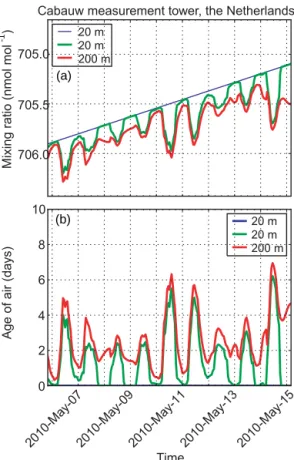
Figure 1 shows the simulated mixing ratios and applied forcing for the tracer “Surface” at the location of the Cabauw tower from 6 to 15 May 2010, together with the derived AoA. We use here output from the TM5 model on 1×1◦resolution (see Table 4). At 20 m above the surface during the night-time, AoA is generally close to zero, due to the fact that the volume is forced in the lowest 100 m, and vertical mixing is limited in a stable nocturnal boundary layer. During the day-time, however, older air from aloft is mixed in, and the AoA increases depending on the depth of the mixing layer and the strength of the vertical mixing. At 200 m, outside the forc-ing volume, air is generally older. Durforc-ing some nights, e.g. from 8 to 9 May, the surface becomes decoupled from the air masses aloft, signalling a stable boundary layer. Note that the depth of the lowest model layer is approximately 20 m, which implies that this layer is entirely within the forcing
Cabauw measurement tower, the Netherlands M ix in g ra tio ( nm ol m ol ) 705.0 705.5 706.0 A ge o f ai r (d ay s) 10 8 6 4 2 0 2010-M ay-07 2010-M ay-09 2010-M ay-11 2010-M ay-13 2010-M ay-15 Time 20 m 20 m 200 m 20 m 20 m 200 m -1 (a) (b)
Figure 1. (a) Mixing ratios of an AoA tracer simulated by the TM5 model (TM5_1x1) forced at the surface along the Cabauw measure-ment tower in the Netherlands during May 2010. The blue line rep-resents the applied forcing. (b) Similar, but transferred to AoA.
volume (the applied forcing is indicated by the blue line). However, TM5 still calculates a non-zero AoA in the low-est model layer because the mixing ratios are sampled af-ter vertical transport, which mixes in older air (Krol et al., 2005). We do not provide recommendations on the sampling strategy. For instance, models that sample right after forc-ing, simulate a linear mixing ratio increase at 20 m (blue line in Fig. 1a) and a constant and zero AoA at 20 m (blue line in Fig. 1b). The current paper will focus on large-scale transport timescales, and we found no major influence of this sampling strategy on the results.
To complement the AoA tracers, modellers were also re-quested to simulate the tracers listed in Table 2. Simula-tions of 222Rn are intended to study vertical and synoptic-scale transport (Jacob et al., 1997); SF6 is used to
diag-nose IH transport, stratosphere–troposphere exchange, and stratospheric AoA; E90 is used to diagnose the “chemical” tropopause and will be compared to Prather et al. (2011). Note that we also included a222Rn simulation with monthly varying emissions over Europe during 2006–2010, based on the high-resolution emission maps presented in Karstens et al. (2015). The current paper will, however, not analyse these simulations.
Homogeneous surface emissions (in kg m−2s−1) of E90 (EE90) are calculated such that the mean steady-state
atmo-spheric mixing ratio of E90 will approach 100 nmol mol−1:
EE90=
Matm×100 × 10−9
τE90×4π r2
, (2)
with Matm the atmospheric mass (kg), r the radius of the
Earth (m), and τE90 the e-folding lifetime (90 days in units
s) of E90.
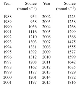
Emissions of SF6 based on EDGAR4.0 (Emission
Database for Global Atmospheric Research) with corrections suggested by Levin et al. (2010) are given in Table 3. The emission distribution is similar to Patra et al. (2011).
NetCDF-formatted input files were provided with emis-sions on 1◦×1◦ resolution and initial SF6 mixing ratios
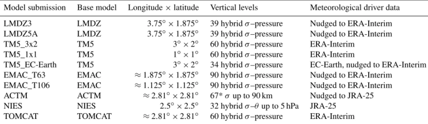
for 1 January 1988. In terms of output, modellers were re-quested to provide monthly mean 3-D mixing ratios and hourly mixing ratio time series at 247 atmospheric mea-surement stations (interpolated or grid value). Furthermore, hourly atmospheric profiles of mixing ratios and meteoro-logical variables (u wind, v wind, surface pressure, bound-ary layer height, geopotential height) were requested at 119 locations. In this first analysis, we will concentrate on the output of monthly mean mixing ratios that have been pro-vided by three CTMs and three GCMs, some of them run-ning in different configurations. Table 4 lists the participat-ing models along with their horizontal and vertical resolu-tion. Three models (LMDZ, EMAC, ACTM) run in “on-line” mode, meaning that meteorology is calculated by the physics module of the model and nudged towards a reanaly-sis dataset, such as ERA-Interim (Dee et al., 2011), provided by the European Centre for Medium-Range Weather Fore-casts and JRA-25 from the Japanese Meteorological Agency (Onogi et al., 2007; Chiaki and Toshiki, 1016). Three other models (TM5, NIES, TOMCAT) run in “offline” mode, and directly read in meteorological driver data from a reanalysis. TM5_Earth reads in meteorological data from the EC-Earth model (Hazeleger et al., 2010) that is nudged to ERA-Interim (see Sect. 2.3)
In the next subsections, specific information on the partic-ipating models and the measurements is given.
2.2 LMDZ
LMDZ, developed at Laboratoire de Météorologie Dy-namique with “Z” standing for zoom capacity, is the global general circulation model of the IPSL Earth system model (Hourdin et al., 2006, 2012). Here, we include two offline versions of LMDZ – LMDZ3 and LMDZ5A –, both with a horizontal resolution of 1.875◦(latitude) ×3.75◦(longitude) and a vertical resolution of 39 hybrid sigma–pressure levels, commonly chosen for global inverse studies using LMDZ (Chevallier, 2015; Locatelli et al., 2015b; Yin et al., 2017). These two versions are different in terms of the physical pa-rameterisation of deep convection and boundary layer
mix-Table 2. Additional tracers in the model inter-comparison. Tracer Remarks
222Rn Radon tracer, similar to Jacob et al. (1997), Law et al. (2008), Patra et al. (2011)
222RnE As222Rn, but with specific monthly emissions over Europe in 2006–2010 (Karstens et al., 2015)
SF6 SF6tracer, similar to Patra et al. (2011), but with updated yearly emissions (Table 3)
E90 Tracer with surface emissions and atmospheric lifetime of 90 days (Prather et al., 2011)
Table 3. Yearly emissions of SF6for the period 1988–2015.
Year Source Year Source
(mmol s−1) (mmol s−1) 1988 934 2002 1223 1989 938 2003 1258 1990 1036 2004 1268 1991 1116 2005 1299 1992 1210 2006 1366 1993 1303 2007 1475 1994 1381 2008 1555 1995 1392 2009 1577 1996 1312 2010 1599 1997 1208 2011 1642 1998 1162 2012 1685 1999 1177 2013 1729 2000 1201 2014 1772 2001 1197 2015 1816
ing. LMDZ3 uses the deep convection scheme of Tiedtke (1989) and the boundary layer mixing scheme of Louis (1979). LMDZ5A is an updated version that uses the deep convection scheme of Emanuel (1991) and the boundary layer mixing parameterisation from Louis (1979), further ad-justed according to Deardorff (1966). More details regarding the configurations of the physics and comparison to other versions are described in Locatelli et al. (2015a). Sea sur-face temperature and sea ice coverage from ERA-Interim are used as boundary conditions. Horizontal winds are nudged towards ERA-Interim wind fields with a relaxation time of 3 h.
2.3 TM5
The TM5 model (Krol et al., 2005) has different application areas with a common core. TM5 allows for a flexible grid definition with two-way nested zoom regions. This version is mainly used in inverse modelling applications, focussing on CO2 (Peters et al., 2010), CH4 (Bergamaschi et al., 2013;
Houweling et al., 2014), and CO (Krol et al., 2013). The chemistry version of TM5 (Huijnen et al., 2010) was recently adapted for massive parallel computing (Williams et al., 2017). The AoA simulations were conducted in this so-called TM5-MP version.
The TM5 model is used in three versions that differ in horizontal resolution and in the way meteorological data are used. The version named TM5_3x2 simulated the AoA ex-periment at a resolution of 3◦×2◦ (longitude × latitude). In the version TM5_1x1, a horizontal resolution of 1◦×1◦
was used. TM5_1x1 and TM5_3x2 refer to simulations with the offline TM5-MP version that reads in the meteorologi-cal fields from files. Like earlier model versions, TM5_1x1 and TM5_3x2 are driven by ERA-Interim and updated every 3 h, with time interpolation during time integration. For this inter-comparison, we include all 60 vertical levels provided by the ECMWF ERA-Interim reanalysis. Convective mass fluxes are derived from entrainment and detrainment rates from the ERA-Interim dataset. This replaces the convec-tive parameterisation used in the previous TransCom inter-comparison (Patra et al., 2011), which was based on Tiedtke (1989). According to Tsuruta et al. (2017) the mass fluxes produced with the ERA-Interim dataset lead to faster inter-hemispheric transport compared to the old model version us-ing the Tiedtke (1989) scheme that was used in the earlier TransCom study (Patra et al., 2011).
The vertical diffusion in the free troposphere is calculated according to Louis (1979) and in the boundary layer by the approach of Holtslag and Boville (1993). Diurnal variabil-ity in the boundary layer height is determined using the pa-rameterisation of Vogelezang and Holtslag (1996). Advective fluxes are calculated using the slopes scheme (Russel and Lerner, 1981), with a refinement in time step whenever the Courant–Friedrichs–Lewy (CFL) criterion is violated.
TM5_EC-Earth is the atmospheric transport model of the earth system model EC-Earth version 3.2.2 (Version 2.3 is described in Hazeleger et al., 2010, 2012) The main dif-ferences between the two versions are an increased resolu-tion (from T159 with 62 vertical layers in version 2.3 to T255 with 91 vertical layers in version 3.2.2) and updated versions of the separate model components. Only the atmo-spheric components are used in this study. The dynamical core of EC-Earth is based on the Integrated Forecasting Sys-tem (IFS), version cy36r4 (Molteni et al., 2011). In con-trast to the offline versions of TM5, the dynamical properties of the atmosphere are simulated by EC-Earth in TM5_EC-Earth. EC-Earth was nudged towards ERA-Interim data for temperature, vorticity, divergence, and the logarithm of the surface pressure. The nudging used a relaxation time of 6 h, allowing for continuous atmospheric dynamics when
follow-Table 4. Short-hand notation of the models participating in this study, along with model information.
Model submission Base model Longitude × latitude Vertical levels Meteorological driver data LMDZ3 LMDZ 3.75◦×1.875◦ 39 hybrid σ –pressure Nudged to ERA-Interim LMDZ5A LMDZ 3.75◦×1.875◦ 39 hybrid σ –pressure Nudged to ERA-Interim
TM5_3x2 TM5 3◦×2◦ 60 hybrid σ –pressure ERA-Interim
TM5_1x1 TM5 1◦×1◦ 60 hybrid σ –pressure ERA-Interim
TM5_EC-Earth TM5 3◦×2◦ 34 hybrid σ –pressure EC-Earth, nudged to ERA-Interim EMAC_T63 EMAC ≈1.875◦×1.875◦ 90 hybrid σ –pressure Nudged to ERA-Interim
EMAC_T106 EMAC ≈1.125◦×1.125◦ 90 hybrid σ –pressure Nudged to ERA-Interim
ACTM ACTM ≈2.81◦×2.81◦ 67* σ up to 90 km Nudged to JRA-25
NIES NIES 2.5◦×2.5◦ 32 hybrid σ –θ up to 5 hPa JRA-25
TOMCAT TOMCAT ≈2.81◦×2.81◦ 60 hybrid σ –pressure ERA-Interim * Only the lower 50 layers have been submitted.
ing the ERA-Interim data. Every 6 h, the meteorological data are transferred via de OASIS3 coupler (Valcke, 2013) to TM5-MP, which uses these data to calculate the actual atmo-spheric transport as described above. Apart from the meteo-rological data, the model code of TM5-EC-Earth is similar to TM5_3x2, but with a reduced number of vertical levels (34, i.e. a subset of the 91 levels used in IFS, instead of 60).
2.4 EMAC
The EMAC (ECHAM/MESSy Atmospheric Chemistry) model employed in this study, combines an updated ver-sion 2.50 of the MESSy (Modular Earth Submodel System) framework (Jöckel et al., 2005, 2010) with version 5.3.02 of the ECHAM5 (European Centre Hamburg) general circula-tion model (Roeckner et al., 2006). The version of the EMAC model used here, first described by Jöckel et al. (2006), in-corporates a recent update to convective transport of tracers (Ouwersloot et al., 2015) and is further improved upon to fa-cilitate the nudging of AoA tracers. These modifications are included in version 2.52 of MESSy.
Dynamical properties are simulated by EMAC itself. The model dynamics are weakly nudged in the spectral space, nudging temperature, vorticity, divergence, and surface pres-sure (Jeuken et al., 1996). Different nudging coefficients are used for different vertical levels, with no nudging in the boundary layer and above ∼ 10 hPa and with maximum nudging in the free troposphere. Convective mass fluxes are diagnosed in the CONVECT submodel (Tost et al., 2006), while the resulting transport is calculated by the CVTRANS model (Tost et al., 2010; Ouwersloot et al., 2015). The sim-ulations with EMAC make use of 90 vertical hybrid sigma– pressure levels. Data are available for two horizontal resolu-tions: T63 (192 × 96 grid) with a fixed time step of 6 min and T106 (320 × 160 grid) with a fixed time step of 4 min.
2.5 ACTM
The CCSR/NIES/FRCGC (Center for Climate System Re-search/National Institute for Environmental Studies/Frontier Research Center for Global Change) atmospheric general cir-culation model (AGCM)-based chemistry transport model (ACTM) has been developed for simulations of long-lived gases in the atmosphere (Numaguti et al., 1997; Patra et al., 2009a, 2014). The ACTM simulations are performed at a horizontal resolution of T42 spectral truncation (∼ 2.8 × 2.8◦) with 67σ levels in the vertical and model top at ∼ 90 km. The horizontal winds and temperature of ACTM are nudged with JRA-25. The nudging forces the AGCM-derived meteorology towards the reanalysed horizontal winds (u and vcomponents) and temperature (T ) with relaxation times of 2 and 5 days, respectively, except for the top and bottom model layers.
The heat and moisture exchange fluxes at the Earth’s sur-face are calculated using inter-annually varying monthly-mean sea ice and sea surface temperature from the Hadley Centre observational data products (Rayner et al., 2003). Tracer advection is performed using a fourth-order flux-form advection scheme comprising of the monotonic piecewise parabolic method (Colella and Woodward, 1984) and a flux-form semi-Lagrangian scheme (Lin and Rood, 1996).
Sub-grid-scale vertical fluxes are approximated using a non-local closure scheme based on Holtslag and Boville (1993) and the level 2 scheme of Mellor and Yamada (1974). The cumulus parameterisation scheme is simplified from Arakawa and Schubert (1974) and used for calculating the updraft and downdraft of tracers by cumulus convection.
2.6 NIES
The NIES Eulerian three-dimensional offline transport model is driven by the JRA-25 dataset. It employs a reduced hor-izontal latitude–longitude grid with a spatial resolution of 2.5◦×2.5◦ near the equator (Maksyutov and Inoue, 1999) and a flexible hybrid sigma–isentropic (σ –θ ) vertical
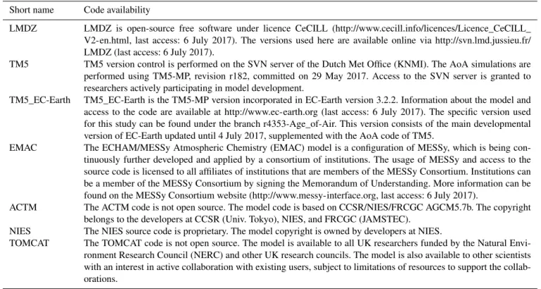
coordi-Table 5. Availability of source code for the models featured in this paper. Short name Code availability
LMDZ LMDZ is open-source free software under licence CeCILL (http://www.cecill.info/licences/Licence_CeCILL_ V2-en.html, last access: 6 July 2017). The versions used here are available online via http://svn.lmd.jussieu.fr/ LMDZ (last access: 6 July 2017).
TM5 TM5 version control is performed on the SVN server of the Dutch Met Office (KNMI). The AoA simulations are performed using TM5-MP, revision r182, committed on 29 May 2017. Access to the SVN server is granted to researchers actively participating in model development.
TM5_EC-Earth TM5_EC-Earth is the TM5-MP version incorporated in EC-Earth version 3.2.2. Information about the model and access to the code are available at http://www.ec-earth.org (last access: 6 July 2017). The specific version used for this study can be found under the branch r4353-Age_of-Air. This version consists of the main developmental version of EC-Earth updated until 4 July 2017, supplemented with the AoA code of TM5.
EMAC The ECHAM/MESSy Atmospheric Chemistry (EMAC) model is a configuration of MESSy, which is being con-tinuously further developed and applied by a consortium of institutions. The usage of MESSy and access to the source code is licensed to all affiliates of institutions that are members of the MESSy Consortium. Institutions can be a member of the MESSy Consortium by signing the Memorandum of Understanding. More information can be found on the MESSy Consortium website (http://www.messy-interface.org, last access: 6 July 2017).
ACTM The ACTM code is not open source. The model code is based on CCSR/NIES/FRCGC AGCM5.7b. The copyright belongs to the developers at CCSR (Univ. Tokyo), NIES, and FRCGC (JAMSTEC).
NIES The NIES source code is proprietary. The model copyright is owned by developers at NIES.
TOMCAT The TOMCAT code is not open source. The model is available to all UK researchers funded by the Natural Envi-ronment Research Council (NERC) and other UK research councils. The model is also available to other scientists with an interest in active collaboration with existing users, subject to limitations of resources to support the collab-orations.
nate, which includes 32 levels from the surface up to 5 hPa (Belikov et al., 2013b). The vertical transport for all levels above the tropopause and higher than a potential temperature level of 295 K follows a climatological adiabatic heating rate. The parameterisation of turbulent diffusivity separates trans-port processes in the planetary boundary layer (provided by the ECMWF ERA-Interim reanalysis) from the free tropo-sphere following the approach by Hack et al. (1993). Vertical mass fluxes due to cumulus convection are based on the con-vective precipitation rate provided by the reanalysis dataset (Austin and Houze Jr., 1973; Belikov et al., 2013a). A mod-ified Kuo-type parameterisation scheme (Grell et al., 1994) is used to set cloud top and cloud bottom height. Transport by convective updrafts and downdrafts includes entrainment and detrainment processes as described by Tiedtke (1989).
2.7 TOMCAT
TOMCAT/SLIMCAT is a global 3-D offline chemical trans-port model (Chipperfield, 2006). It is used to study a range of chemistry–aerosol–transport issues in the troposphere (e.g. Monks et al., 2017) and stratosphere (e.g. Chipperfield et al., 2015). The model is usually forced by ERA-Interim, al-though GCM output can also be used. When using ECMWF fields, as in the experiments described here, the model reads in the 6-hourly fields of temperature, humidity, vorticity, di-vergence, and surface pressure. The resolved vertical motion is calculated online from the vorticity. The model has differ-ent options for the parameterisations of sub-grid-scale tracer
transport by convection (Stockwell and Chipperfield, 1999; Feng et al., 2011) and boundary layer mixing (Louis, 1979; Holtslag and Boville, 1993). Tracer advection is performed using the conservation of the second-order moment scheme of Prather et al. (1987). For the experiments the model was run at a horizontal resolution of 2.8◦×2.8◦with 60 hybrid σ–pressure levels from the surface to ∼ 60 km. These follow the vertical levels from the meteorological fields from ERA-Interim, which are used to force the model. Convective mass fluxes were diagnosed online using a version of the Tiedtke scheme (Stockwell and Chipperfield, 1999) and mixing in the boundary layer is based on the local scheme of Louis (1979). Previous work with the model has shown that these schemes tend to underestimate the mixing out of the bound-ary layer and convective transport to the upper troposphere (e.g. Feng et al., 2011), but these were the options available for the multi-decadal runs analysed here.
2.8 Measurement data
We will compare model results to latitudinal SF6gradients
measured by the National Oceanic & Atmospheric Admin-istration Earth System Research Laboratory (NOAA/ESRL) (Hall et al., 2011). We use the combined dataset con-structed from flask data measured by the Halocarbons and other Atmospheric Trace Species (HATS) group and hourly Chromatograph for Atmospheric Trace Species (CATS) data (downloaded from https://www.esrl.noaa.gov/gmd/hats/ combined/SF6.html, last access: 6 July 2017) and include
P ressur e (hP a) LSCE_LMDZ5A TM5_3x2 EMAC_T63 ACTM_T42L67 NIES TOMCAT Latitude -50 0 +50 Latitude -50 0 +50 Days Surface 90 75 60 45 30 15 0 100 300 500 700 900 100 300 500 700 900 100 300 500 700 900
Figure 2. Zonally averaged AoA (days) in the troposphere for the tracer “Surface”. The results have been averaged over the period 2000–2010 (11 years). The light grey areas correspond to the zonal mean orography in the models. The thin black lines denote the mid-pressure levels of the models. For reference, the dotted black line in all panels denotes the climatological tropopause (Lawrence et al., 2001). The white areas correspond to areas in which the air is older than 100 days.
only stations with a full measurement record in the period 2000–2011. To account for model–data offsets, 11-year time series with monthly resolution were constructed of the sta-tions’ mixing ratios with respect to the South Pole. The mean and standard deviations of these time series are added to the modelled latitudinal gradients below.
In Appendix A we further compare the simulated SF6
lat-itudinal and vertical gradients to measurements made dur-ing the High-performance Instrumented Airborne Platform for Environmental Research (HIAPER) Pole-to-Pole Obser-vation (HIPPO) campaigns (Wofsy et al., 2011), similar to comparisons presented in Patra et al. (2014).
3 Results
3.1 Tropospheric AoA
First, we focus on zonal and multi-year averages to investi-gate differences among the models in IH and vertical trans-port in the troposphere. We created these averages by (i) av-eraging the monthly mean mixing ratios of the participating models zonally and over time and (ii) converting the mean mixing ratios to AoA. These latitude–pressure cross sections are presented in Fig. 2 for the AoA tracer Surface and in Fig. 3 for the AoA tracers “NHsurface” and “SHsurface” (see Table 1).
The AoA in the troposphere derived from the tracer Sur-face is generally younger than 100 days (Fig. 2). The 100-day contour sharply marks the transition to the stratosphere at around 300 hPa at the poles. In the tropics this transition is located at a pressure lower than 100 hPa, which generally agrees with the definition of the climatological tropopause given by Lawrence et al. (2001). Deep convective transport drives the vertical transport in the tropics, and this deep con-vective region is bounded by tongues of older air, signalling intrusions of stratospheric air (Holton et al., 1995). Although all models agree on this general pattern, clear differences are also present. Deep convective mixing in the tropics is strongest in ACTM, while TOMCAT and NIES generally show slower vertical transport and larger AoA gradients be-tween the surface and the upper troposphere.
The tracers NHsurface (Fig. 3a) and SHsurface (Fig. 3b) are used to diagnose IH transport. Generally, the air at high latitudes has an age of between 0.6 and 1.2 years in the hemi-sphere opposite to the forcing volume. Here, all models agree on an interesting asymmetry: AoA derived from SHsurface around the North Pole is 0.10–0.17 years older than AoA derived from NHsurface around the South Pole. TOMCAT, diagnosed with slow vertical mixing, has older air at high latitudes, while NIES (also slow vertical mixing) has high-latitude ages more in line with other models, indicating fast horizontal transport near the surface. Figure 3 illustrates the fact that the exchange of air between the hemispheres pro-ceeds faster at higher altitudes (200–500 hPa) (Prather et al., 1987), and consequently steep AoA gradients are observed close to the surface in the tropics.
3.2 AoA derived from the “Land” and “Ocean” tracers
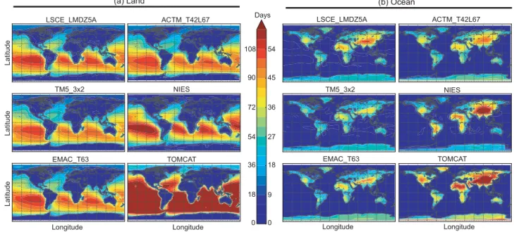
Figure 4 shows AoA derived from the tracers Land (panel a) and Ocean (panel b) evaluated at the lowest model level. Oldest air related to last contact with land is found over the Southern Ocean, with ages older than 100 days. Models gen-erally agree on the fact that old air is found in the station-ary high-pressure areas over the ocean that are related to the Hadley and Walker circulations. This agrees qualitatively with previous findings using the E90 tracer (Prather et al., 2011). The TOMCAT model, in the configuration used here, has systematically larger AoA at the surface. Dominant land– ocean transport patterns are easily discerned from the simu-lations with the Land tracer. Young air over oceans is found south-east of South America, north-west of Australia, and to-wards the north-east of North America and Asia, associated with the position of the upper-air jet stream. The oldest air in the southern east Pacific for the tracer Land indicates that this region is most isolated from the NH emissions. In accor-dance with this, the lowest CH4mixing ratios on the Earth’s
surface are found at the NOAA site Easter Island (EIC). Pa-tra et al. (2009b) attributed these to “old” air in combination with the strong removal of CH4by OH at tropical latitudes.
LSCE_LMDZ5A TM5_3x2 EMAC_T63 ACTM_T42L67 NIES TOMCAT Latitude -50 0 +50 Latitude0 +50 -50 1.26 1.05 0.84 0.63 0.42 0.21 0.00 Years P ressur e (hP a) LSCE_LMDZ5A TM5_3x2 EMAC_T63 ACTM_T42L67 NIES TOMCAT Latitude -50 0 +50 Latitude -50 0 +50
(a) NH_surface (b) SH_surface
100 300 500 700 900 100 300 500 700 900 100 300 500 700 900
Figure 3. Zonally averaged AoA (years) in the troposphere for the tracers “NHsurface” (a) and “SHsurface” (b). The results have been averaged over the period 2000–2010 (11 years). The light grey areas correspond to the zonal mean orography in the models. The white areas correspond to regions in which the air is older than 1.4 years.
54 45 36 27 18 9 0 LSCE_LMDZ5A TM5_3x2 EMAC_T63 ACTM_T42L67 NIES TOMCAT Longitude Longitude 108 90 72 54 36 18 0 LSCE_LMDZ5A TM5_3x2 EMAC_T63 ACTM_T42L67 NIES TOMCAT Latitude Longitude Latitude Latitude Longitude Days
(a) Land (b) Ocean
Figure 4. Latitude–longitude plot of the AoA (days) derived from the tracers “Land” (a) and “Ocean” (b), evaluated in the lowest model layer. The results have been averaged over the period 2000–2010 (11 years). Ages older than 120 days (land tracer) or 60 days (ocean tracer) appear in dark red.
The AoA derived from the tracer Ocean (Fig. 4b) gener-ally shows ages less than 60 days over land, with the older ages logically located in deep inland areas. Its AoA over land is strongly determined by dominant circulation patterns such as the monsoon, trade winds, and jet streams. Although these patterns are similar in all models, the spread is considerable, with TOMCAT again showing the oldest air and TM5 show-ing the youngest air over land surfaces. These differences are
related to the boundary layer parameterisations in the models and in the case of TOMCAT the use of the simple local Louis (1979) scheme. Earlier studies (Wang et al., 1999; Chipper-field, 2006) revealed that this type of local boundary layer (BL) mixing scheme leads to a slower exchange between the BL and the free atmosphere.
3.3 Stratospheric AoA
We use the tracer Surface to compare the simulated strato-spheric AoA. Here, it should be noted that differences in tropospheric mixing influence the results. For instance, the TOMCAT and NIES AoA are systematically older at the tropopause (see Fig. 2). Figure 5 shows the stratospheric AoA for all models from 100 hPa to the top of the atmo-sphere, averaged over the period 2000–2010 (11 years). As expected, the oldest AoA is found at the high-altitude poles. Considerable model spread is found with the oldest air (up to 7 years) in LMDZ5A and the youngest air in ACTM (< 5 years). The transport in EMAC, TOMCAT, LMDZ, and TM5 is driven by – or nudged to – ERA-Interim meteo-rology (see Table 4), and one would expect similar spheric AoA in these models. However, AoA in the strato-sphere is not only determined by the driving meteorological data but also by the treatment of advection (specifically tical transport), nudging parameters, and the number of ver-tical layers in the model (Prather et al., 2008). According to a stratospheric AoA study by Diallo et al. (2012), the use of instantaneous wind fields at 3- or 6-hourly time intervals in CTMs may under-sample fast vertical variations during these time intervals. For GCMs that are nudged to reanal-ysis meteorological data, gravity wave noise may influence the stratospheric AoA. Finally, the vertical coordinate sys-tem may influence numerical transport effects (Chipperfield, 2006; Diallo et al., 2012). Other studies on stratospheric AoA (Garny et al., 2014; Ploeger et al., 2015) highlighted the importance of separating stratospheric mixing into a (slow) residual circulation and (fast) eddy mixing. Further analysis on the stratospheric AoA in this model ensemble is, however, left for future exploration.
3.4 Inter-hemispheric transport
In this section, we compare the inter-hemispheric transport times using the tracers NHsurface and SHsurface to the sim-ulated latitudinal gradients of SF6. To this end, we show in
Fig. 6a the simulated zonal average latitudinal SF6
gradi-ent at the surface. All gradigradi-ents have been scaled relative to the South Pole SF6 mixing ratio. Also included in the
fig-ure are the latitudinal gradients measfig-ured by NOAA/ESRL (Hall et al., 2011). Since the selected model results are av-erages over all longitudes, including the land masses with high emissions, modelled zonal averages exceed the observa-tions at NH midlatitudes. Most notably, high-altitude staobserva-tions such as Niwot Ridge (3523 m above sea level (m a.s.l.)) and Mauna Loa (3397 m a.s.l.) show much smaller mixing ratio differences with respect to the South Pole than, for example, Cape Kumukahi at sea level. This is confirmed by panel (b) of Fig. 6, in which the modelled SF6fields are zonally
av-eraged over the Pacific Ocean only (from 150 to 210◦E). In this average all models except NIES agree well within 0.1 pmol mol−1 on the latitudinal gradient. Due to too
re-P ressur e (hP a) LSCE_LMDZ5A TM5_3x2 EMAC_T63 ACTM_T42L67 NIES TOMCAT Latitude -50 0 +50 Latitude -50 0 +50 Years 6.30 5.25 4.20 3.10 2.10 1.05 0.00 0 20 40 60 80 100 0 20 40 60 80 100 0 20 40 60 80 100 Surface
Figure 5. Zonally averaged AoA (years) in the stratosphere for the tracer Surface. The results have been averaged over the period 2000–2010 (11 years). The thin black lines denote the mid-pressure levels of the model. For the ACTM model, this level is at around 17 hPa for the uppermost 50th layer. The dotted black line denotes the climatological tropopause. Note the linear y scale that starts at 100 hPa.
duced a vertical mixing combined with fast latitudinal trans-port, the NIES model underestimates the latitudinal SF6
gra-dient. The TOMCAT model simulates the observed latitudi-nal gradient of SF6 on clean background stations well but
also shows high accumulation over land (see Figs. 4 and 6a). In Appendix A we further compare the simulated SF6
lati-tudinal and vertical gradients to measurements made during the HIPPO campaigns (Wofsy et al., 2011).
Panel (c) of Fig. 6 depicts a composite of the AoA of the tracer NHsurface at the SH surface and of the tracer SHsur-face at the NH surSHsur-face. Again, all results are zonal averages over 2000–2010 (11 years) and include all longitudes. Panel (d) of Fig. 6 confirms the NH–SH asymmetry noted earlier in Sect. 3.1 but also makes it clear that the asymmetry dif-fers with model. Panel (d) of Fig. 6 highlights the NH–SH asymmetry by subtracting the NHsurface AoA sampled at the SH surface from the SHsurface AoA sampled at the NH sur-face. In all models, differences grow gradually from 10◦ lat-itude to the pole, where the AoA differences range between 0.10 years (TM5_3x2) and 0.17 years (EMAC_T106). The model versions with higher spatial resolution (TM5_1x1, EMAC_T106) show larger AoA differences compared to the lower-resolution versions. The TM5_EC-Earth version dif-fers from the other TM5 versions, likely because the physics of the EC-Earth model (IFS version cy36r4) leads to differ-ences in boundary layer mixing and convection, compared to the IFS model version that was used for the ERA-Interim simulation (cy31r2).
-50 0 +50 Latitude 0.8 0.6 0.4 0.2 S F 6 (p m ol m ol ) re la tiv e to S ou th P ol e 0.0 0.4 0.3 0.2 0.1 0.0 A ge o f ai r (y ea r) 1.2 1.0 0.8 0.6 0.4 -50 0 +50 Latitude spo cgo smo kum mlo nwr mhdbrw alt spo cgo smo
kum
mlo nwr mhd brw alt
Pacific Ocean zonal average Zonal average over all longitudes (a) (b) (c) (d) 0.20 0.10 0.15 0.05 0.00 -0.05 -0.10 0.25 A ge o f ai r N -S d iff er en ce ( ye ar ) | Latitude | 10 20 30 0 40 50 60 70 80 90 LSCE_LMDZ3 LSCE_LMDZ5A TM5_3x2 TM5_1x1 TM5_EC_Earth EMAC_T63 EMAC_T106 NIES ACTM_T42L67 TOMCAT -0.15 -1
Figure 6. Panels (a) and (b): latitudinal gradient of SF6(pmol mol−1) at the surface, averaged over 2000–2010 (11 years). Panel (a) includes
all longitudes in the modelled zonal average, while panel (b) includes only longitudes over the Pacific Ocean (150 to 210◦E). Modelled gradients have been scaled with respect to the South Pole. The grey symbols and their variability are calculated from the combined dataset constructed from flask data measured by the HATS group from NOAA/ESRL and hourly CATS data (https://www.esrl.noaa.gov/gmd/hats/ combined/SF6.html, last access: 6 July 2017). Three-letter codes refer to the stations (alt: Alert, Canada; brw: Pt. Barrow, Alaska, USA; mhd: Mace Head, Ireland; nwr: Niwot Ridge, Colorado, USA; kum: Cape Kumukahi, Hawaii, USA; mlo: Mauna Loa, Hawaii, USA; smo: Cape Matatula, American Samoa; cgo: Cape Grim, Tasmania, Australia; spo: South Pole). Variability is calculated as the standard deviation of monthly time series of the station data relative to the South Pole station. Panel (c): composite of the AoA (years) of the tracer NHsurface at the SH and the tracer SHsurface at the NH (see main text; averaged over 2000–2010). Panel (d): AoA difference (years) calculated from the values of panel (c). The AoA at the SH of the tracer NHsurface is subtracted from the AoA at the NH of the tracer SHsurface and plotted against latitude.
From Fig. 6a and c it is obvious that the TOMCAT model shows the strongest SF6 gradient, along with the slowest
IH transport as diagnosed from the tracers NHsurface and SHsurface. NIES shows smaller SF6 gradients but IH AoA
values in line with other models. Differences between the other models are less pronounced. The gradient of SF6 is
driven by emissions that take place mainly at midlatitude land masses in the NH. In contrast, the tracers NHsurface and SHsurface are forced at the entire surface of both hemi-spheres. To make a meaningful comparison to the simulated latitudinal gradients of SF6, we evaluate the AoA of the
trac-ers NHsurface and SHsurface at 50◦S and 50◦N, respec-tively, and at the surface of the models. By adding these two ages, we align the resulting composite AoA with the bulk of the calculated latitudinal SF6gradient between the South
Pole and 50◦N in panel (b) of Fig. 6. The result is shown in Fig. 7. In this representation, the NIES model deviates by simulating weaker latitudinal SF6gradients. TOMCAT
sim-ulates a similar SF6gradient compared to other models but
differs in the composite AoA. Both models have weak ver-tical mixing (see Fig. 2), but NIES has fast horizontal trans-port, while TOMCAT accumulates SF6 over the source
re-gions over land (see Fig. 6a). Different model versions
clus-ter together in this representation, but differences between the LMDZ5A and LMDZ3 are larger. This illustrates the impact of the parameterisation of convective mixing in the LMDZ models (see Sect. 2.2).
3.5 Vertical transport
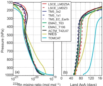
In this section, we focus on the vertical transport in the tropo-sphere, as diagnosed from the tracer Land and the simulated vertical gradients of222Rn. To this end, we show in Fig. 8a the simulated mean vertical profiles, area-weighted between 60◦S and 60◦N on a log scale. Clearly, the TOMCAT and NIES models retain the222Rn closer to the surface because of slower vertical mixing. The other models mix the222Rn to higher altitudes, but larger differences are found at pressures smaller than 400 hPa, where some models exhibit stronger increases at 150–300 hPa (e.g. ACTM, LMDZ5A), associ-ated with the parameterisation of convective mixing. Fig. 8b shows the vertical profiles of the AoA of the tracer Land, averaged in the same manner.
To investigate the consistency of differences in vertical mixing between the models, Fig. 9 compares the simulated vertical gradient in222Rn to the simulated AoA profiles of
2.2 2.1 2.0 1.9 1.8 1.7 C omposit e A oA (y ear) 1.6
SF6 gradient 50° N - South Pole (pmol mol )
0.25 0.30 0.35 0.40 0.45
-1
Figure 7. Composite AoA (years) plotted against the modelled SF6 gradient. The composite AoA is calculated as the sum of the 50◦N AoA of the tracer SHsurface and the 50◦S AoA of the tracer NHsur-face. The SF6gradient is taken as the concentration difference
be-tween 50◦N and the South Pole from Fig. 6b. Results are averaged over 2000–2010 (11 years).
the tracer Land. Because222Rn decays radioactively with a half-life of 3.8 days, we convert the vertical gradient of222Rn mixing ratio as
1 =ln222Rn(950 hPa) − ln222Rn(500 hPa), (3) where we do not sample directly at the surface to avoid dif-ferences in sampling strategies between models (see Sect. 2). Here, we quantify the gradient with respect to the 500 hPa level. In Fig. 9 we plot the AoA gradient between 500 and 950 hPa against 1. The results of the different models show a high degree of linear correlation, indicating that models with efficient vertical mixing (e.g. TM5, ACTM) have small AoA differences between the boundary layer and 500 hPa along with a flatter222Rn profile. Models with slow vertical mixing (NIES, TOMCAT) show steeper 222Rn profiles along with larger 1 values. Interestingly, the TM5 and EMAC mod-els show that higher spatial-resolution modmod-els lead to faster vertical mixing. This is different to the results found for IH transport and likely due to the fact that deep convective mix-ing is a scale process. Numerics of such sub-grid-scale processes are less prone to numerical diffusion com-pared to the advection process that drives the IH gradient. As expected, the two model versions of LMDZ that differ by their convective parameterisation show distinct differences in the vertical profiles.
3.6 Mapping the tropopause
Prather et al. (2011) introduced an idealised tracer (E90) to delineate the boundary between troposphere and stratosphere in transport models. Driven by surface emissions and a de-cay rate of 90 days−1, tracer E90 is meant to quantify the
P ressur e (hP a) 100 200 300 400 500 600 700 800 900 1000
222Rn mixing ratio (mol mol )
-21 -20 -19
10
10 10
Land AoA (days)
0 40 80 120 160 LSCE_LMDZ5A LSCE_LMDZ3 TM5_3x2 TM5_1x1 TM5_EC_Earth EMAC_T63 EMAC_T106 ACTM_T42L67 NIES TOMCAT -1 (a) (b)
Figure 8. Vertical profiles of 222Rn (a, mol mol−1, logarithmic axis) and the AoA of the Land tracer (b, in days) simulated by the different models. The vertical profiles have been area-weighted-averaged between 60◦N and 60◦S and over the years 2000–2010 (11 years).
rate of mixing of tropospheric air. Through numerical ex-periments, the tropopause in the UCI CTM (Prather et al., 2011) was defined as the surface on which the mixing ratio of E90 is 90 nmol mol−1. Note that emissions of E90 are de-fined such that the global stationary state concentration of E90 is 100 nmol mol−1 (see Sect. 2). Mixing ratios in the stratosphere are lower, due to the long transport times. As an alternative to E90, the AoA tracer Surface may also be used to delineate the stratosphere from the troposphere, as shown in Fig. 2. In order to compare the tropopause pressure calculated by either E90 or the AoA surface tracer, we plot the tropopause pressure as a function of latitude in Fig. 10. The tropopause pressure is calculated based on 2000–2010 zonal averages of E90 (unit nmol mol−1) and Surface AoA (unit days). For each latitude the tropopause pressure is de-termined by interpolation to E90 = 90 nmol mol−1 (dotted lines in Fig. 10) and to Surface AoA = 90 days (solid lines in Fig. 10). Results show consistency for these two met-rics, although larger differences occur for several models. Differences in tropopause pressure based on E90 and the tracer Surface are likely caused by the transport character-istics of the models. The Surface AoA simulation is forced by linearly increasing boundary conditions which are con-verted to AoA, while the E90 simulation is driven by sur-face emissions and a decay process with a 90-day turnover time. This causes different tracer gradients and hence a dif-ference in advective and convective transport. As a result, ACTM calculates systematically higher tropopause pressures for E90, while for NIES the reverse is observed. Other mod-els show similar estimates for both tracers. When modmod-els are compared, both tracers calculate similar tropopause pressure
Ln( Rn) 950 hPa–Ln( Rn) 500 hPa
1.2
1.4
1.6
1.8
2.0
2.2
222 222 A oA (500 hP a) - A oA (950 hP a) (da ys)50
45
40
35
30
25
20
15
Figure 9. The 500–950 hPa difference in AoA (days) of the Land tracer plotted against 1: a measure for the vertical gradient in222Rn (see main text). The vertical profiles used for the calculations are shown in Fig. 8.
differences, with NIES showing a very deep tropopause at higher latitudes and TOMCAT a shallower tropopause. Of-fline models that use the same driver meteorological data (e.g. TOMCAT and TM5) would be expected to have a sim-ilar tropopause based on common temperature fields. How-ever, since the tropopause pressures derived here depend on the transport of tracers by advection and convection, substan-tial differences are found that also depend on the choice of concentration (for tracer E90) and AoA (for the tracer Sur-face) at which the tropopause is evaluated. Finally, all models agree on a hemispheric asymmetric average tropopause with a tropopause pressure maximum around 55◦S, likely
asso-ciated with an enhanced stratosphere–stratosphere exchange in the SH (Holton et al., 1995). In most models, this pressure maximum is more pronounced for tracer E90.
4 Discussion
This TransCom AoA inter-comparison shows that the tropo-spheric AoA concept provides useful information on model transport characteristics. It was shown that the IH transport timescale in a particular model is strongly connected to the efficiency of vertical mixing and hence to the specific imple-mentation of sub-grid-scale convective transport. Thus, the AoA metric may be used to better understand flux differ-ences derived from CO2and CH4flux inversions (Law et al.,
2008; Patra et al., 2011). The NIES model, which has slow convective mixing, still shows fast IH mixing, a small IH SF6 gradient, and a deep extra-tropical tropopause. In
con-trast, the TOMCAT model in the configuration used here combines weak vertical mixing with a stronger SF6
gradi-ent between land and ocean and a shallower tropopause. The
P ressur e (hP a) 50 100 150 200 250 300 350 -50 0 +50 Latitude LSCE_LMDZ5A TM5_3x2 EMAC_T63 ACTM_T42L67 NIES TOMCAT
Figure 10. Zonal average tropopause pressure (averaged over 2000– 2010) as a function of latitude, obtained from the AoA tracer Sur-face (solid lines) and E90 (dashed lines) for different models (see legend). Tropopause pressure is obtained from 1-D linear interpo-lation to 90 days for the AoA tracer Surface and to 90 nmol mol−1 for E90.
TM5 model, which was diagnosed with slow IH transport in the TransCom methane inter-comparison (Patra et al., 2011), now uses the convective fluxes stored in the ECMWF ERA-Interim archive, which are based on Gregory et al. (2000) and other changes (Tsuruta et al., 2017; Dee et al., 2011). This brings the IH transport times close to other models (see Fig. 7). This confirms the fact that the parameterisa-tion of sub-grid convective fluxes in CTMs deserves atten-tion, specifically when used in atmospheric inversion stud-ies. This is in line with the study of Stephens et al. (2007), who showed that the attribution of the global CO2land sink
depends strongly on the vertical mixing in models.
We found an interesting hemispheric asymmetry in the IH transport times, with “older” NH air diagnosed with an AoA tracer forced at the SH surface, compared to the age of SH air, diagnosed with an AoA tracer forced at the NH surface. We tentatively attribute this asymmetry to the effect of land masses in the NH, which lead to an atmospheric stabilisa-tion in winter, decoupling the BL from the overlying free troposphere (FT). In the AoA protocol, this affects the sur-face forcing. The situation is reversed in summer, with more efficient mixing over land masses. The resulting net effect is well known as the “seasonal rectifier” (Denning et al., 1995). In Appendix B we present a simplified numerical experiment that shows that the mean AoA in the upper atmosphere short-ens with a larger seasonal cycle in near-surface mixing, in line with the asymmetry in IH transport as found in all mod-els. Thus, the AoA metric can also be used to quantify the strength of these rectifier effects in CTMs. Another (related)
factor that might be responsible for this asymmetry is the mean position of the intertropical convergence zone (ITCZ) north of the equator (Schneider et al., 2014).
A further important timescale in GCMs and CTMs is the mixing time of the BL and its coupling with the overlying FT. Together with the aforementioned “convection” timescale, these two quantities appear responsible for the main model diversity in this inter-comparison. For instance, the TM5 model shows a relatively strong coupling between the BL and the FT, witnessed by (i) relatively young air of the Ocean AoA tracer over land (Fig. 4), (ii) only a small IH difference in the AoA (Fig. 6d), and (iii) a small 950–500 hPa verti-cal gradient in222Rn and the Land AoA tracer (Fig. 9). Dif-ferences with the EMAC, LMDZ, and ACTM models seem to be determined by the strength of this BL–FT coupling. Differences with NIES and TOMCAT, however, seem to be driven by differences in the convective parameterisation.
Other model differences, such as resolution, advection scheme, the meteorological driver data, nudging, and the ver-tical coordinate system may also play a role and may become more apparent on the smaller spatial and temporal scales that are not part of this first analysis. In mapping the tropopause with either E90 or the AoA derived from the surface tracer (Fig. 10), model-dependent differences appeared that may be related to the treatment of atmospheric transport. AoA tracers with a linearly growing boundary condition lead to different concentration gradients than tracers with surface emissions and first-order decay, such as E90. In regions with large gradients, such as the planetary boundary layer and the tropopause, differences in the numerical treatment of advec-tion may lead to different transport characteristic of AoA tracers, compared to tracers with physical sources and sinks. Our multi-model results agree qualitatively with the study of Waugh et al. (2013) that focused on SF6and an AoA tracer
in a single model (GMI-MERRA). They found older AoA than the age derived from SF6observations. The AoA
sim-ulations presented here allow for more detailed analyses in the future, including comparisons to earlier efforts to quan-tify tropospheric AoA based on observations (e.g. Holzer and Waugh, 2015).
The simple AoA concept exploited here is easily imple-mented in CTMs and GCMs, and other modellers are en-couraged to implement AoA tracers in their models. The AoA protocol is also useful as a benchmark for model de-velopment, similar to Prather et al. (2008). Analysis of AoA simulations performed with a single model with different ad-vection schemes, convective parameterisations, or nudging schemes can be used to study their impact on large-scale transport features, such as IH and vertical transport. AoA studies with a single transport model and different meteoro-logical driver data (e.g. ERA-Interim versus JRA-25) would reveal the potential role of the meteorological driver data on AoA biases. Finally, the entire time series (1988–2015) may be used to study trends in the Brewer–Dobson circulation (Fu et al., 2015) or IH transport timescales.
5 Conclusions
This paper presents the first results of the TransCom AoA inter-comparison. Six models simulated five AoA tracers and four additional tracers over the time period 1988–2015. AoA tracers were forced by linearly growing boundary conditions in a predefined atmospheric volume. Advantages of this ap-proach are that (i) the forcing volume can be flexibly cho-sen and (ii) transport timescales can easily be derived based on simulated mixing ratios that indicate when an air mass was last in contact with the boundary. Disadvantages are that (i) there are no known atmospheric species with linear grow-ing boundary conditions and (ii) artificial mixgrow-ing ratio gra-dients introduced close to the forcing volume may be chal-lenging for advection schemes. Successful implementation of the protocol in six global models revealed interesting dif-ferences in large-scale transport features. In this paper we mainly analysed averages over the 2000–2010 period. The main findings of this study are as follows:
1. The inter-hemispheric transport time depends strongly on the strength of the convective parameterisation in the participating models. Although convective mixing is identified as a major cause for inter-model differ-ences, other causes, such as the source of reanalysis data, nudging, and advection scheme, cannot be ruled out at the moment. It is recommended to apply the AoA protocol in a single model with different set-ups to study the impact on large-scale transport features.
2. Inter-hemispheric transport proceeds faster from the NH to the SH than from the SH to the NH. This is at-tributed to the seasonal rectifier effect caused by NH land masses, with strong mixing in summer and weak mixing in winter as shown in Appendix B.
3. Boundary layer mixing and venting to the free tropo-sphere over land varies among models, which leads to consistent differences in modelled vertical gradients. The TM5 model shows fast vertical mixing, with conse-quently relatively young air of the Ocean AoA tracer over land (Fig. 4). In contrast, the TOMCAT model shows slow vertical mixing and old air of the Ocean AoA tracer over land.
4. The AoA concept can be used to map the tropopause. At the tropopause the air has last been in contact with the surface 90 days ago (AoA = 90 days). For most models, the derived tropopause pressure is in good agreement with the E90 tracer (Prather et al., 2011).
5. Upper-stratospheric AoA varies considerably among the participating models (4–7 years).
In general, further analysis is required to fully exploit the simulations presented in this paper. For instance, the analy-sis of inter-annual variations in inter-hemispheric transport and stratospheric AoA may reveal interesting differences be-tween the models. Most of all, further analysis should fo-cus on the causes of the still large spread in the participating models.
Code availability. The AoA protocol and analysis software in the form of a Jupyter Notebook (Python) are available to the com-munity through github (https://github.com/maartenkrol/AoA) and are available at https://doi.org/10.23728/b2share.d6849238d65f435 c8f022221f2107cdd (Krol et al., 2018). The Python notebook aoa_paper.ipynb needs AoA_tools.py. The model output, converted to a standard format, can be downloaded from the ftp location men-tioned in AoAprotocol.pdf. Apart from the AoA tracers discussed in this paper, AoA tracers are also available that are forced in the troposphere and stratosphere. These tracers are forced above and below a climatological pressure surface given by Lawrence et al. (2001). Results are not discussed because not all models used the correct definition. Information on the availability of source code for the models featured in this paper is given in Table 5.
Appendix A: Comparison with HIPPO SF6
Figure A1 compares monthly mean SF6 output from the
models to observations made during the HIPPO campaigns (Wofsy et al., 2011). Only HIPPO flights over the Pacific Ocean are included, and the corresponding model mixing ratios are averaged over the Pacific Ocean only (from 150 to 210◦E). Hippo 1 observations are compared to monthly means of January 2009, Hippo 2 to November 2009, Hippo 4 to June and July 2011 averages, and Hippo 5 to August 2011. Panel (a) shows the latitudinal gradients averaged over 1– 3 km. Since models used different SF6 1988 mixing ratios
as initial fields and show different accumulation rates in the lower atmosphere, models have been shifted to match the 2009 observations. Note that the shifts (mentioned in the caption) range from +1.3 ppt for TOMCAT to −0.4 ppt for NIES. During the 2009–2011 HIPPO period differences be-tween these two models gradually increase further. This is likely related to fast accumulation in NIES due to limited vertical mixing, combined with fast horizontal transport in the lower atmosphere. TOMCAT was also diagnosed with
Gradient -1 -1 Gradient -1 Gradient -1 Gradient -1 -1 -1 -1 -1 -1 -1 -1 -1 -1 (a) (b)
Figure A1. Comparison of modelled monthly-mean SF6(averaged over the Pacific Ocean only, from 150 to 210◦E) to the High-performance
Instrumented Airborne Platform for Environmental Research (HIAPER) Pole-to-Pole Observation (HIPPO) campaigns (Wofsy et al., 2011), similar to comparisons presented in Patra et al. (2014). Panel (a) show models and observations averaged over 1–3 km altitude. Panel (b) shows the gradient between 5–7 km averages and 1–3 km averages. Models have been shifted to match the HIPPO latitudinal gradients in 2009. Magnitudes of the shifts are indicated in the caption.
slow vertical transport (see Fig. 2) but also with slow hor-izontal mixing (signalled by old air over the ocean for the AoA tracer Land in Fig. 4). Other models agree on a faster increase in SF6 in the models compared to observations,
signalling a likely overestimate of the emissions in 2009– 2011 (see Table 3). The latitudinal gradients are very similar among the models (except for NIES as in Fig. 6) and gen-erally agree well with observations. Figure A1b shows the modelled and measured vertical SF6gradients, calculated by
taking the difference between 5–7 km averages and 1–3 km averages, as in Patra et al. (2014). Modelled and measured vertical gradients are very small and measurement noise pre-vents us from drawing firm conclusions about the ability of models to correctly simulate SF6vertical gradients.
Appendix B: Seasonal rectifier effect
The intention of this Appendix is to calculate the effect of seasonal vertical mixing over land on the calculated mean AoA in the upper atmosphere. In the main paper it is spec-ulated that a seasonal rectifier effect partly explains why the AoA derived from SHsurface around the North Pole in the models is 0.10–0.17 years older than AoA derived from NHsurface around the South Pole (Fig. 6d). With more land cover, seasonality in mixing is stronger in the NH com-pared to the SH. To illustrate the seasonal rectifier effect, we implemented the AoA protocol in a simplified three-box model. To this end, we force a surface three-box of 100 m (pressure difference 1p1 between bottom and top: 13 hPa)
with a linearly growing mixing ratio as a boundary condi-tion. The surface box mixes with an overlying boundary layer box (1p2=137 hPa). This boundary layer box additionally
mixes with the overlying free atmosphere (1p3=600 hPa).
Mixing timescales between the boundary layer and the forced surface layer (τ1), and between the boundary layer and free
atmosphere (τ2) vary with season according to
τ1= (a1sin(2π t ) + 1.0) 1 365, (B1) τ2= (a2sin(2π t ) + 1.0) 7 365, (B2)
where time t is measured in years and a1and a2are the
am-plitudes of the seasonal cycles imposed on the standard mix-ing timescales τ1 and τ2of 1 and 7 days, respectively. The
following set of differential equations is solved to simulate the mixing ratios x1, x2, and x3according to the AoA
proto-col: dx1 dt =1, dx2 dt = x1−x2 τ1 −x2−x3 τ2 , dx3 dt = 1p2 1p3 x2−x3 τ2 , where 1p2
1p3 accounts for the fact that boxes 2 and 3 have
dif-ferent pressure thicknesses. We now performed two simu-lations: one representing the SH with no seasonal cycle in mixing (a1=a2=0) and one representing the NH, with a
50 % amplitude in seasonal mixing (a1=a2=0.5). Results
of the simulations, with mixing ratios converted into AoA units (AoA = t − x), are plotted in Fig. B1a. As expected, NH AoA (solid lines) shows a seasonal cycle in the bound-ary layer and free atmosphere, while the SH simulation (dot-ted lines) reaches a steady-state AoA in the free atmosphere of about 37 days, roughly in line with the multi-year aver-aged AoA of the tracer Surface in Fig. 2. Figure B1b shows the percentage difference in the 1-year moving average of the NH and SH simulations, calculated as 100 ×SH−NHNH . In-deed, the average AoA in the free atmosphere and boundary
(a)
(b)
Figure B1. Panel (a): simulated AoA in the simple three-box model described in the main text. The solid lines show the NH simula-tion with a 50 % seasonal cycle in vertical mixing. The dotted lines show the SH simulation with no seasonal cycle in vertical mixing. Panel (b): difference in the 1-year moving average AoA calculated as 100 ×SH−NHNH .
layer is younger by about 3 % when a seasonal cycle is ap-plied to the vertical mixing. Thus, even when the mean mix-ing timescales between the boxes are the same, the resultmix-ing mean AoA in the upper atmosphere is different. In a real at-mosphere, other factors may also play a role, such as con-vection and the asymmetry in the mean position of the ITCZ north of the equator (Schneider et al., 2014). Nevertheless, this simple example shows that a rectifier effect may partly explain the asymmetry in inter-hemispheric mixing as seen in all models (Fig. 3).