HAL Id: hal-03165188
https://hal-amu.archives-ouvertes.fr/hal-03165188
Submitted on 10 Mar 2021HAL is a multi-disciplinary open access archive for the deposit and dissemination of sci-entific research documents, whether they are pub-lished or not. The documents may come from teaching and research institutions in France or abroad, or from public or private research centers.
L’archive ouverte pluridisciplinaire HAL, est destinée au dépôt et à la diffusion de documents scientifiques de niveau recherche, publiés ou non, émanant des établissements d’enseignement et de recherche français ou étrangers, des laboratoires publics ou privés.
Phytoplankton distribution from Western to Central
English Channel, revealed by automated flow cytometry
during the summer-fall transition
Arnaud Louchart, Fabrice Lizon, Alain Lefebvre, Morgane Didry, François
Schmitt, Luis Felipe Artigas
To cite this version:
Arnaud Louchart, Fabrice Lizon, Alain Lefebvre, Morgane Didry, François Schmitt, et al.. Phyto-plankton distribution from Western to Central English Channel, revealed by automated flow cytom-etry during the summer-fall transition. Continental Shelf Research, Elsevier, 2020, 195, pp.104056. �10.1016/j.csr.2020.104056�. �hal-03165188�
1
Please note that this is an author-produced PDF of an article accepted for publication following peer review. The definitive publisher-authenticated version is available on the publisher Web site.
Continental Shelf Research
April 2020, Volume 195, Pages 104056 (16p.) https://doi.org/10.1016/j.csr.2020.104056 https://archimer.ifremer.fr/doc/00601/71324/
Archimer
https://archimer.ifremer.fr
Phytoplankton distribution from Western to Central English
Channel, revealed by automated flow cytometry during the
summer-fall transition
Louchart Arnaud 1, *, Lizon Fabrice 1, Lefebvre Alain 2, Didry Morgane 1, 3, Schmitt François G. 1,
Artigas Luis Felipe 1, *
1 Univ. Littoral Côte D’Opale, Univ. Lille, CNRS, UMR 8187, LOG, Laboratoire D’Océanologie et de
Géosciences, F 62930, Wimereux, France
2 IFREMER, LER/BL, Boulogne sur Mer, France
3 Aix Marseille Univ., Université de Toulon, CNRS, IRD, MIO, UM110, 13288, Marseille, France
* Corresponding authors : Arnaud Louchart, email address : arnaud.louchart@gmail.fr ; Luis Felipe Artigas, email address : felipe.artigas@univ-littoral.fr
Abstract :
Automated pulse shape-recording flow cytometry was applied to address phytoplankton spatial distribution, at high frequency, in stratified and well mixed water masses in the Western and Central English Channel during the summer-fall transition. Cytometric pulse shapes derived from optical features of single cells allowed the characterization of eight phytoplankton groups. Abundance and total red fluorescence (chlorophyll a autofluorescence) per group were used to define six phytoplankton communities. Their distribution revealed high spatial heterogeneity. Abundance presented a longitudinal gradient for six over the eight groups and succession of brutal shifts along the cruise. Maximum values were often located near the Ushant front in the Western English Channel. A latitudinal gradient characterized the Central English Channel waters under the influence of the Seine estuary. Picophytoplankton (Synechococcus-like cells and picoeukaryotes) represented up to 96% of total abundance and half of the total red fluorescence of the communities near the main front and the Bay of Seine, whereas nanoeukaryotes and microphytoplankton, represented only 4% and less than 1% respectively of total abundance. Both nanoeukaryotes and microphytoplankton dominated the total red fluorescence of the communities of the Central English Channel. The study of traits within each group showed a high variability of traits between communities. The comparison between traits showed that they were independent from each other for some groups (size and red fluorescence per cell for PicoHighFLR and Coccolithophore-like cells; orange and red fluorescence for all the groups), whereas they were dependent for other groups (red fluorescence per cell was dependent of size for picophytoplankton, NanoLowFLR, NanoHighFLR, Cryptophyte-like cells and Microphytoplankton). Variance partitioning revealed that the environmental parameters (temperature, salinity and turbidity) accounted less than spatial descriptors (physical and biological processes) in shaping the communities. Hydrological structures (frontal structures, eddies and tidal streams) were responsible for patches of phytoplankton and defined the structure at the sub-mesoscale (1 – 10 km) in this area.
2
Please note that this is an author-produced PDF of an article accepted for publication following peer review. The definitive publisher-authenticated version is available on the publisher Web site.
Highlights
► Automated flow cytometry addresses phytoplankton community changes at high frequency. ► Eight cytometric groups are characterized from pico-to microphytoplankton size range. ► Variation in cytometry-derived traits can be characterized between communities. ► Frontal structures drive phytoplantkon spatial distribution at sub-mesoscale.
Keywords : English Channel, phytoplankton distribution, high resolution, automated flow cytometry,
1. Introduction
52
Carbon uptake and fixation through photosynthesis (Falkowski, 1994; Falkowski et al., 1998; Gregg et 53
al., 2003) make phytoplankton account for up to 50% of the annual global net primary production, 54
while its biomass only represents 2% of the total global biomass (Falkowski et al., 2003; Field et al., 55
1998). Furthermore, phytoplankton are involved in many biogeochemical cycles (Falkowski, 1994; 56
Falkowski et al., 1998; Gregg et al., 2003) and in most of the marine food webs being a prey for 57
grazers affecting growth, cellular processes and community composition (Holligan and Harbour, 1977; 58
Lampert et al., 1986; Rassoulzadegan et al., 1988). Given the importance of phytoplankton in marine 59
ecosystems, there is a consequent need to perform accurate estimates of abundance and biomass 60
(which are also defined as biological descriptors in the Marine Strategy Framework Directive (MSFD 61
2008/56/EC) and Water Framework Directive (2000/60/EC) in order to understand the populations 62
assembly into different communities and how these communities influence/determine biogeochemical 63
cycles as well as higher trophic levels (e.g. Falkowski et al., 1998; Litchman, 2007; Litchman et al., 64
2007). The large size-range and diversity of phytoplankton characterise high variations of 65
surface/volume ratios as well as physiological capacities, leading to a different capacity of growth 66
among phytoplankton, sometimes dividing twice a day (Alpine and Cloern, 1988). In addition, 67
environmental drivers are often episodic, contributing to quick changes of phytoplankton responses 68
over space and time scales. Current monitoring sampling strategies might fail to detect these responses 69
(Pearl et al., 2007). Therefore, a trade-off in phytoplankton sampling strategies is needed in order to 70
understand the determinism of phytoplankton changes and distribution, considering both fine space 71
and time scales and environmental parameters. 72
Considering the techniques available, the use of microscopy and HPLC pigment analysis provide, 73
respectively, high taxonomical and pigmentary composition. However, they are not suitable for high 74
space and time resolution studies (Cullen et al., 1997; Millie et al., 1997; Richardson and Pinckney, 75
2004) because of the time-consuming and highly specialised work to be carried out back at the 76
laboratory. On the other hand, despite in vivo fluorometry could reach a reliable space and time 77
coverage (Rantajärvi et al., 1998), it provides only bulk measurements as estimates of total chlorophyll 78
a (as a proxy of phytoplankton biomass). Several innovative techniques (e.g. multispectral 79
fluorometry, automated flow cytometry, remote sensing) have shown to give representative insights 80
into phytoplankton composition (at least at the functional level), abundance and/or chlorophyll a at 81
high resolution (Bonato et al., 2015; De Monte et al., 2013; Lefebvre and Poisson-Caillault, 2019; 82
Marrec et al., 2018, 2014; Thyssen et al., 2015). Among these techniques, automated “pulse shape-83
recording” flow cytometry (PSFCM) addresses almost the whole phytoplankton size-range (c.a. from 84
less than 1µm to 800 µm width) at single-cell or single-colony level and characterizes them based on 85
their combined or integrated optical properties (i.e. light scattering, fluorescence; Dubelaar et al., 86
2004, 1999). Indeed, this technique records the entire pulse shape of a single particle (Rutten et al., 87
2005; Thyssen et al., 2008b, 2008a), from small cells as Prochlorococcus-like (Marrec et al., 2018) up 88
to large cells and/or colonies of diatoms or Phaeocystis globosa (Bonato et al., 2016, 2015; Rutten et 89
al., 2005). Moreover, the cytometric optical properties provide useful proxies of cell length, width, 90
morphology, internal composition and physiology which can be assimilated to functional derived 91
traits. Therefore, the variation of phytoplankton traits at high frequency remain to be investigated 92
across the different spatial scales. 93
The Western and Central part of the English Channel are well-documented areas which benefit from 94
sustained monitoring (e.g. Astan Buoy, Astan & Estacade SOMLIT stations, L4 and E1 stations; 95
Eloire et al., 2010; Goberville et al., 2010; Not et al., 2004; Smyth et al., 2010; Sournia et al., 1987). 96
This epicontinental sea is strongly impacted by climate variability (Goberville et al., 2010) making 97
seasonal and interannual variation in the hydrological and climatic conditions responsible of changes 98
in plankton communities composition (Foulon et al., 2008; Marie et al., 2010; Tarran and Bruun, 99
2015; Widdicombe et al., 2010). In the Western English Channel (WEC), from May to October, the 100
hydrological conditions go from well-stratified to well-mixed conditions and shape the position of the 101
Ushant tidal front (Pingree and Griffiths, 1978). Eddies that bring high nutrient concentrations in 102
addition to the light, make communities accumulating along the front, especially diatoms and 103
dinoflagellates, and contribute to high biomass (Landeira et al., 2014; Pingree et al., 1979, 1978, 104
1977). Moreover, the geostrophic flow, eddies, wind upwelling and tidal streams occur along the front 105
allowing phytoplankton dispersion and crossing the front (Pingree et al., 1979). Therefore, the front 106
extends on scales from meters to kilometres (d’Ovidio et al., 2010; Ribalet et al., 2010). In the Central 107
English Channel (CEC), both the English and the French coast are influenced by river run-off. In the 108
French part, the Seine River contributes to form permanent halocline stratification (Brylinski and 109
Lagadeuc, 1990; Menesguen and Hoch, 1997). During the late summer-fall period, the Bay of Seine is 110
initially characterised by high abundance of diatom (Jouenne et al., 2007). Then, when the depletion of 111
nutrient occurs in summer, diatom abundance decrease and dinoflagellate abundance increase (Thorel 112
et al., 2017). Along the English coast, the Southampton Water estuarine system contributes largely to 113
enhance nutrients along the coast (Hydes and Wright, 1999). Nutrients are especially brought by the 114
Test and Itchen rivers, which drain agricultural land as well as sewage discharge effluents (Hydes and 115
Wright, 1999) resulting in chlorophyll a peaks in spring and summer (Iriarte and Purdie, 2004; Kifle 116
and Purdie, 1993; Leakey et al., 1992). 117
Despite most of phytoplankton studies in the English Channel concerned the coastal areas (e.g. Hydes 118
and Wright, 1999; Iriarte and Purdie, 2004; Jouenne et al., 2007; Marie et al., 2010; Not et al., 2004; 119
Pannard et al., 2008; Smyth et al., 2010; Tarran and Bruun, 2015; Widdicombe et al., 2010), some of 120
them concerned coastal-offshore gradients focusing both in the Eastern English Channel (EEC, Bonato 121
et al., 2016, 2015; Lefebvre and Poisson-Caillault, 2019), Central English Channel (WEC, Napoléon 122
et al., 2014, 2012) and Western English Channel (Garcia-Soto and Pingree, 2009; Marrec et al., 2014, 123
2013; Napoléon et al., 2013) (Garcia-Soto and Pingree, 2009; Marrec et al., 2014, 2013; Napoléon et 124
al., 2014, 2013, 2012). Some attempts were carried out on transects crossing the English Channel in 125
the WEC and CEC (Garcia-Soto and Pingree, 2009; Marrec et al., 2014, 2013; Napoléon et al., 2013). 126
However, these studies reflected three major drawbacks: first of all, some transects were carried out 127
along a latitude gradient, missing the longitude component in which spatial gradients are particularly 128
known to occur in the English Channel (Napoléon et al., 2014, 2013, 2012). Secondly, most of them 129
resulted in a spatial aliasing by missing any fine spatial scale variability. Finally, these spatiotemporal 130
studies mainly sampled the largest organisms (> 20 µm) of the phytoplankton compartment, missing 131
most of the picophytoplankton and the small nanophytoplankton (< 20µm) fraction. 132
In the present study, we analyse the spatial distribution of some phytoplankton size- and optically-133
defined functional groups as well as their assembly in communities, highlighting the relation between 134
environmental and spatial features with phytoplankton communities’ variability, addressed at high 135
frequency, on a high spatial sampled gridded area. Phytoplankton single-cells and colonies were 136
characterised by continuous recording of sub-surface pumped seawater, by using an automated “pulse 137
shape-recording” flow cytometer coupled to continuous recording hydrological features. With a high 138
resolution spatial sampling strategy, our aims were: (i) to study the phytoplankton distribution per 139
functional group and the variation of the traits within each group across space with respect to meso- to 140
sub-mesoscale hydrological features as frontal areas (ii) to identify the key environmental and spatial 141
variables that could explain the variability between communities’ composition and (iii) to define the 142
scale of variability of phytoplankton communities among sites. 143
2. Materials and methods
144
2.1 Cruise outlines
145
Samples were collected during a multidisciplinary cruise focusing on an ecosystemic end-to-end 146
approach of fisheries in the Western English Channel. The CAMANOC (CAmpagne MANche 147
OCcidentale, Travers-Trolet and Verin, 2014) cruise took place on board the RV Thalassa (Ifremer) 148
from the 16th of September to the 16th of October 2014, during the summer-fall transition. The ship 149
crossed the English Channel from West to East (Fig. 1). A Pocket-FerryBox system (PFB, 4H-JENA) 150
was coupled to a pulse shape-recording flow cytometer (PSFCM, CytoSense, Cytobuoy), a 151
thermosalinometer (SeaBird SBE21) and an in vivo fluorometer (Turner Designs 10-AU). In vivo 152
fluorometer required a two steps calibration. The first one used a blank water (de-ionized water) and 153
the second one used a solid standard. The water intake was at the front of the ship’s cooling system at 154
a fixed depth (4 m), and in normal ship operation seawater is constantly pumped. The PFB was 155
assembled with sensors for salinity and temperature (Seabird 45 micro TSG), and turbidity (Seapoint). 156
Seawater was pumped at 4 m depth and was continuously analysed by all the sensors. The acquisition 157
of data was continuously performed, and we obtained an integration of the measurement from 1 158
minute (PFB) to 10 minutes (PSFCM). Because of a relatively brief transit time of water from the 159
water intake to PFB, the observations are representative of sub-surface conditions. The lower 160
resolution was kept to merge phytoplankton functional features with environmental data. The ship 161
navigated at the speed of 11 knots for 1 month. This led to a resolution of approximately 3.4 km (for 162
automated flow cytometry) with a total of 2910 samples, considering stops for discrete fisheries, 163
benthos, plankton and hydrological sampling. 164
166
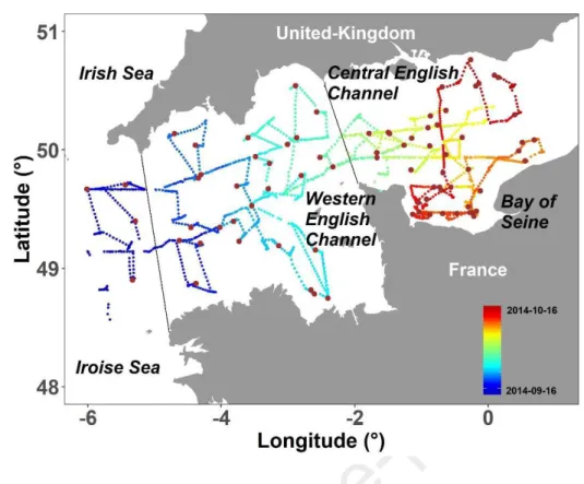
Figure 1: Continuous recording every 10 minutes by a pulse shape-recording flow cytometer (PSFCM) 167
during the CAMANOC cruise from Sept. 16th (blue dots) to Oct. 16th (red dots) and 78 discrete (CTD) 168
stations (brown dots). Dashed lines correspond to geographical separation of the main regions: Celtic 169
Seas (including Irish and Iroise Sea), Western English Channel and Central English Channel. 170
171
2.2 Stratification and mixing of water masses
172
CTD (Seabird SBE 21) casts (78) were performed during the cruise. Temperature (°C), salinity, 173
density (kg.m-3) and depth (m) were recorded at a rate of 1 measure per second. We used the density 174
from the CTD casts to calculate the squared of buoyancy frequency, N² (s-2; 3), in order to quantify the 175
vertical density gradient throughout the water column which quantifies the stratification: 176
(3) N² ≡ g/ρ0 × (δρ(z) / δz) 177
where g (m.s-2) is the acceleration due to gravity, ρ0 (1026 kg.m -3
)is seawater reference density, 178
δρ (kg.m-3) is the density differential along the water column and δz is the depth of the water column, 179
between surface and bottom. 180
2.3 Plankton analysis
181
Continuous pumped waters as well as discrete samples were analysed by a CytoSense (Cytobuoy b.v., 182
Netherlands), an automated flow cytometer (FCM) with the ability of recording the entire optical pulse 183
shape of each particle (“pulse shape-recording flow cytometer”: PSFCM). Five signals compose a 184
particle optical profile. The forward scatter (FWS) is collected via a PIN photodiode whereas the 185
sideward scatter (SWS) and three types of fluorescence: red fluorescence (FLR: 668-734 nm), orange 186
fluorescence (FLO: 604-668 nm) and yellow fluorescence (FLY: 536-601 nm) are collected via a 187
photomultiplier. The instrument uses a solid-state laser (Coherent Inc, 488 nm, 50 mV) to analyse, 188
count and characterise single-cells and colonies (Dubelaar et al., 2004; Pomati et al., 2013; Pomati and 189
Nizzetto, 2013) from 1 µm to 800 µm width and a few mm length (Dubelaar et al., 1999). Each 190
particle passes through a 5 µm laser beam at a speed of 2 m s-1. A trigger-level was used on the red 191
fluorescence (FLR) in order to separate phytoplankton and non-fluorescent particles (Thyssen et al., 192
2015). Continuous recording was performed with this configuration and the trigger-level was set at 15 193
mV during 9 min at a flow rate of 4.5 µL s-1. The clustering was performed manually with the 194
CytoClus software (Cytobuoy b.v., www.cytobuoy.com). The determination of each group was 195
processed considering the amplitude and the shape of the five signals, referring also to previous work 196
on automated flow cytometry in this area (Bonato et al., 2016, 2015; Thyssen et al., 2015) and 197
according to bead size calibration. In addition, the CytoClus software provides several statistical 198
features on each signal (e.g. Length, Total, Average...) as well as the distribution of the different 199
populations of events. The length of the FWS was used as a proxy for cell size. A standardisation of 200
each particle from each cluster was carried out with calibrated beads of 3µm. Two thresholds were set 201
up: the first around 3µm in order to separate picoeukaryotes from nanoeukaryotes and the second 202
around 20 µm in order to separate nanoeukaryotes from microphytoplankton. A group was named 203
according to its estimated size and to its pigmentary features. Following Bonato et al. (2015) particle 204
size was corrected with the measured length FWS of the beads (1 & 2). 205
(1) Correction factor = real beads size / Measured beads size 206
(2) Estimated particles size (µm) = Measure particles size × Correction factor 207
Based on the common vocabulary for automated FCM (available at https://www.seadatanet.org), we 208
characterised 6 main functional groups by automated flow cytometry: Synechococcus-like cells, 209
picoeukaryotes, nanoeukaryotes, Cryptophyte-like cells, Coccolithophore-like cells and 210
Microphytoplankton. In addition, sub-groups were characterised within the picoeukaryotes and 211
nanoeukaryotes groups, according to their red fluorescence’s level. Finally, we defined three 212
picophytoplankton groups (<3µm): Synechococcus-like cells, PicoLowFLR, PicoHighFLR; four 213
nanoeukaryotes groups (3 to 20µm): Cryptophyte-like cells, Coccolithophore-like cells, NanoLowFLR 214
and NanoHighFLR; and one microphytoplankton group (>20µm; Fig. 2). 215
216
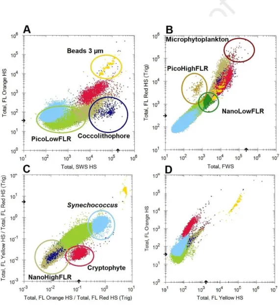
Figure 2: Cytograms allowing the characterisation of different phytoplankton groups. (A) Total 217
Orange Fluorescence (TFLO) vs. Total Sideward Scatter (Total SWS). (B) Total Red Fluorescence 218
(TFLR) vs. Total Forward Scatter (Total FWS). (C) Ratio of Total Yellow Fluorescence over Total 219
Red Fluorescence and Total Orange Fluorescence over Total Red Fluorescence 220
(TFLY/TFLR)/(TFLO/TFLR). (D) Total Orange Fluorescence (TFLO) vs. Total Yellow Fluorescence 221
(TFLY). Clusters of single, doubles and triples of beads of 3 µm are merged here. 222
2.4 Statistical analysis and mapping
223
We considered the environmental parameters (i.e. temperature, salinity and turbidity) and in vivo total 224
fluorescence obtained either by the thermo-salinometer (temperature and salinity), the PFB (turbidity) 225
and the Turner fluorometer (in vivo total fluorescence) to compute a hierarchical classification analysis 226
based on Euclidean distance. A hierarchical classification was computed also for cytometric groups, 227
separately, to characterize the similarity between the phytoplankton communities among the sites. We 228
used scaled data to detect the similarity among the relative changes in community composition, and 229
we computed the Jaccardized Czekanowski similarity index (also known as quantitative Jaccard). In 230
most recent studies on the spatial distribution of phytoplankton, the common procedure is a 231
computation of Bray-Curtis dissimilarity matrix to define communities (Legendre and Legendre, 232
1998). However, Bray-Curtis generates a semi-metric matrix which is not as strong as the quantitative 233
Jaccard which generates a metric matrix for cluster analysis. Thus, the Jaccardized Czekanowski index 234
would be more suitable than Bray-Curtis for similarity studies (Schubert and Telcs, 2014). This 235
distance was computed per phytoplankton feature (i.e. abundance, red fluorescence) calculated from 236
the cytometric groups such as described in Bonato et al., (2015) in order to get the similarity between 237
pairs of samples. We processed the computation of an average similarity matrix between a matrix 238
based on abundance and a matrix based on red fluorescence. This method is more reliable than using 239
them separately because abundance and red fluorescence (proxy of chlorophyll content which in turn 240
is used as a proxy of biomass) are considered as the main features to discriminate the communities. 241
Each function was weighted between 0 and 1. Abundance accounted for 0.5 as well as red 242
fluorescence. We coupled the final similarity matrix with the Ward method (Ward, 1963) which 243
consist in aggregating at each step the two clusters with the minimum within-cluster inertia and detect 244
the homogeneity of the clusters. Then, the optimal classification cut level was obtained by selecting 245
the maximum average silhouette over the Cophenetic distances. These analyses were processed using 246
the packages “vegan”, “analogue” and “cluster” on R. The importance of environment and space 247
(defined as the Euclidean distance between a pair of latitude and longitude coordinates) for structuring 248
phytoplankton communities was studied among each community by processing a variation partitioning 249
(Borcard et al. 1992, Peres-Neto et al. 2006). In our model, the total variance is represented by four 250
fractions [a + b + c + d] where [a +b] represents the environmental fraction; [b + c] represents the 251
space fraction; [b] is the interaction between environment and space and [d] the residual variance. 252
Space was redefined by the calculation of the principal coordinates of neighbour matrices (PCNM, 253
Borcard and Legendre, 2002) to define them as spatial descriptors of the relationship among sampling 254
units. We used the pcnm function from the “vegan” package design for R environment. Phytoplankton 255
communities were detrended using the Hellinger transformation which is appropriate for 256
compositional data by reducing the impact of rare events which are more susceptible to sampling error 257
(Legendre and Gallagher, 2001). In addition, transformation of the data will give the same weight to 258
rare or very abundant groups. Partitions were tested by ANOVA over 999 permutations. Finally, we 259
carried out a multivariate Mantel correlogram to investigate the relationship between geographical 260
distance extracted from the latitude-longitude coordinates and phytoplankton communities over the 261
water bodies. This analysis allowed the detection of the minimal distance at which the correlations 262 disappear. 263 3. Results 264 3.1 Hydrobiology 265
Each continuous-recorded physical variable as well as in vivo total fluorescence (µg equivalent of 266
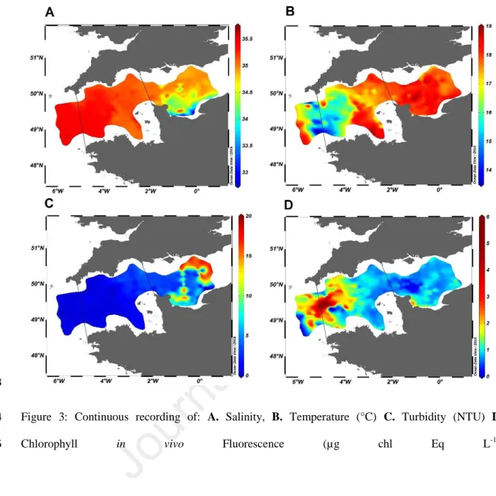
chlorophyll a per L) showed a strong spatial structure. The highest salinity values were recorded in the 267
Western English Channel (35.5; WEC) and decreased moderately towards the East (35). In the Central 268
English Channel (CEC) salinity strongly decreased from 35 in offshore waters to 33 in the inner part 269
of the Bay of seine (BOS; Fig. 3A). Colder waters characterised the entrance of the WEC and were 270
surrounded by warmer waters both in the Celtic Seas as well as in mid WEC waters (Fig. 3B). Sharp 271
transitions were evidenced (of only a few kilometres) both at the West and East of the colder area. 272
273
Figure 3: Continuous recording of: A. Salinity, B. Temperature (°C) C. Turbidity (NTU) D. 274
Chlorophyll in vivo Fluorescence (µg chl Eq L-1).
The highest turbidity values were recorded in the CEC, both in offshore and coastal waters (Fig. 3C). 276
A sharp increase in chlorophyll in vivo fluorescence was evidenced from the outer shelf to the WEC 277
(values shifted from around 0.1 µg chl Eq L-1 to 5.7 µg chl Eq L-1). Then, fluorescence levels 278
decreased rapidly eastward in WEC (from 5.7 µg chl Eq L-1 to 1-1.5 µg chl Eq L-1; Fig. 3D). Spearman 279
ranks correlation were negative and significant with temperature (ρ = -0.45, p<0.001) and turbidity 280
(ρ = -0.29, p<0.001) whereas Spearman rank correlation between fluorescence and salinity was 281
positive and significant (ρ = 0.31, p<0.001). 282
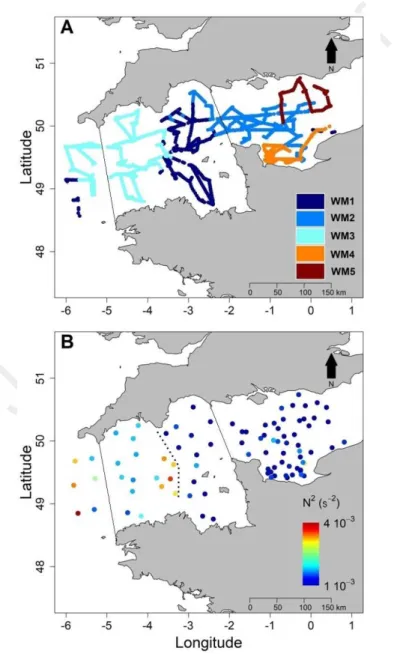
Applying hierarchical clustering on the similarity matrix revealed 5 water masses (WM) in the English 283
Channel (Fig. 4A). Mapping these water masses revealed that Western and Central English Channel 284
were structured in hydrological blocks. WM1 corresponded to the eastern part of the Western English 285
Channel and Celtic Seas out of the Channel (Iroise and Irish Seas), whereas WM3 was located in 286
between, in the centre of the WEC. WM2 was located in offshore waters mainly in the CEC. WM4 287
was under the influence of the Bay of Seine and WM5 was considered as mainly corresponding to the 288
English coastal and offshore waters of the CEC. 289
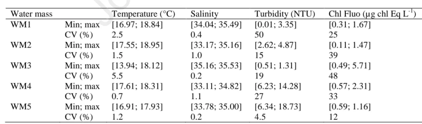
Table 1: Minimum and maximum values of temperature, salinity, turbidity and in vivo chlorophyll 290
fluorescence (Chl Fluo) among the 5 water masses. 291
Water mass Temperature (°C) Salinity Turbidity (NTU) Chl Fluo (µg chl Eq L-1) WM1 Min; max [16.97; 18.84] [34.04; 35.49] [0.01; 3.35] [0.31; 1.67] CV (%) 2.5 0.4 50 25 WM2 Min; max [17.55; 18.95] [33.17; 35.16] [2.62; 4.87] [0.11; 1.47] CV (%) 1.5 1.0 15 39 WM3 Min; max [13.94; 18.12] [35.16; 35.53] [0.51; 1.31] [0.49; 5.71] CV (%) 5.5 0.2 19 48 WM4 Min; max [17.61; 18.31] [33.11; 34.82] [6.23; 14.28] [0.57; 2.31] CV (%) 0.7 1.1 27 33 WM5 Min; max [16.91; 17.93] [33.78; 35.00] [6.34; 18.73] [0.59; 1.16] CV (%) 1.2 0.2 4.5 12 292
The lowest temperature was recorded in the WM3 revealing also the strongest gradient (∆T = 4.18°C, 293
Fig.3B and table 1) whereas this water mass exhibited high stable salinity thus the lowest salinity 294
gradient (∆SAL = 0.37, Fig.3A and table 1) among the water masses. The opposite pattern was 295
observed in the WM1, WM2, WM4 and WM5, the difference of temperature was comprised between 296
0.70°C (WM4) and 1.87°C (WM1) with higher values than in WM3 whereas the salinity difference 297
was comprised between 1.22 (WM5) and 1.99 (WM2) with lower values than in the WM3. Turbidity 298
was also lower in WM3 than in any other WM and showed a small difference (∆TURB = 0.8 NTU). 299
The highest range of turbidity values were found in the WM4 and WM5 (respectively ∆TURB = 8.05 300
NTU and ∆TURB = 12.39 NTU), both WM under the influence of the Solent (UK) and Seine (France) 301
estuaries. In WM3, in vivo chlorophyll fluorescence (Chl Fluo) was higher than in any other water 302
mass and showed the highest variability (∆Chl Fluo = 5.22 µg chl Eq L-1). 303
304
Figure 4: A. Identification of water masses based on results from the Euclidean distance matrix on 305
temperature, salinity, turbidity and in vivo chlorophyll fluorescence. B. Stratification, value of N², as 306
derived from CTD casts. The dashed line distinguishes homogeneous water masses from 307
heterogeneous water masses and marks the front. 308
309
On the West of the main frontal structure (WEC, Fig. 4B), corresponding to WM3, N² values were 310
higher and displayed more heterogeneous waters than in the East side (CEC and BOS), where the 311
values of N² were lower and displayed homogeneous waters. In the WEC (WM3), N² values reached 312
up to 10-3 s-2 whereas in the CEC and the BOS (WM2, WM4 and WM5), the order of magnitude of N² 313
values was between 10-4 and 10-5 s-2 (Fig. 4B). In the Celtic seas, the N² was recorded between 3.5 and 314
4.5 10-3 s-2 decreasing sharply eastward with the shift of temperature to reach 1.5 10-3 s-2 in the WEC. 315
They define the outer thermal front as well as the western limit between WM1 and WM3. Then a 316
second change occurred between the WEC and the CEC. The values of the N² in WM3 of up to 4.0 10 -317
3
s-2 shifted to 10-4 /10-5 s-2 the CEC (WM2, WM4) and the BOS (WM5) defining the inner thermal 318
front. 319
3.2 Phytoplankton abundance, fluorescence and spatial distribution.
320
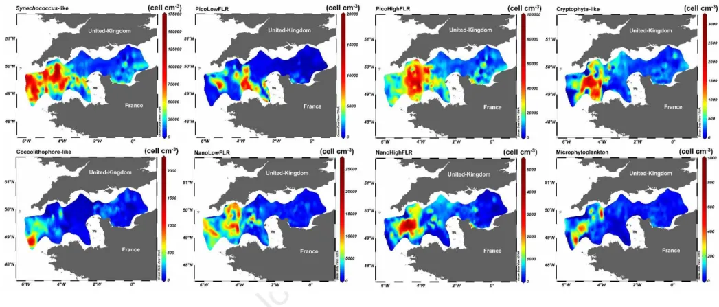
Picoeukaryotes (PicoLowFLR and PicoHighFLR) and Synechococcus-like cells dominated the 321
phytoplankton abundance. They were structured along a decreasing West-East longitudinal gradient 322
but showing an important heterogeneity in spatial distribution (Fig. 5). High abundance was recorded 323
in the Western English Channel (mostly in WM3) whereas low values were recorded in the Central 324
English Channel and, for Picoeukaryotes, at the western entrance of the English Channel (Celtic Seas, 325
Fig. 5 and 6). However, the abundance of Synechococcus-like cells was high out of the Channel and in 326
the WEC, and low in the CEC (Fig. 5A). PicoLowFLR abundance exhibited patches reaching more 327
than 1 × 10⁴ cell mL-1 in the WEC (5% of the highest abundance were representing 950 km2) and close 328
to the Channel isles (Fig. 5B). PicoHighFLR (Fig. 5C) and Cryptophyte-like cells (Fig. 5D) showed 329
the same patterns: low abundance out of the English Channel, sharp increase and high abundance in 330
the WEC (both coastal and offshore waters, WM3), then a sharp decrease and low abundance in the 331
eastern WEC and CEC. Coccolithophore-like cells (Fig. 5E) exhibited high abundance out of the 332
Channel (western WM1), while the abundance remained low elsewhere. NanoLowFLR (Fig. 5F) 333
showed several patches of high abundance (5% of the highest abundance represented 1000 km2) 334
between the limits of WM3 (out of the Channel and in the WEC). In the CEC and BOS, the abundance 335
was low. NanoHighFLR high abundance was also detected in WM3, forming a large patch in offshore 336
waters of the WEC (Fig. 5G), decreasing westward and eastward, showing an increase in a restricted 337
area in the Bay of Seine. Microphytoplankton abundance (Fig. 5H) was low out of the English 338
Channel. Then, patches of high abundance were observed in western WM3, in offshore waters of the 339
WEC. In the CEC and BOS, the abundance was low. 340
The abundance of each group was compared with respect to the distance of the inner WEC thermal 341
tidal front used as an arbitrary geographical reference (Ushant front, Fig. 6). Samples located to the 342
West of the front were represented by a negative distance whereas samples located to the East of the 343
front were represented by a positive distance. A global view revealed that abundance increased as the 344
sample got collected closer to the Ushant frontal area (Fig. 6). This was the case for PicoHighFLR 345
(Fig. 6.C), Cryptophyte-like cells (Fig. 6.E), and NanoLowFLR (Fig. 6.F). On the other hand, 346
NanoHighFLR (Fig. 6.G.) and Microphytoplankton groups (Fig. 6.H.) showed maximum abundance 347
slightly offset (westward) of the front (microphytoplankton also showing high values all along the 348
front). For these groups (PicoHighFLR, Cryptophyte-like cells, NanoLowFLR, NanoHighFLR and 349
Microphytoplankton), the highest levels of abundance were recorded in WM3 which is the most stable 350
water mass observed here. PicoLowFLR (Fig. 6.B), Synechococcus-like cells and Coccolithophore-351
like cells showed a different pattern. The first two groups exhibited high abundance along and across 352
the front in the Western English Channel and in the Celtic Seas (Fig. 6.A) whereas Coccolithophore-353
like cells showed highest abundance only in shelf waters at the western entrance of English Channel 354
(Fig. 6.D) where waters remained warm and stable (outer front of the WEC). At the East of the inner 355
front, the abundance decreased slowly to reach low values at 100 km from the main frontal system 356
(Fig. 6). At 200 km from the front, a second increase of abundance was observed (Fig. 6) for some 357
groups. A Synechococcus-like cells (Fig. 6.A.), PicoLowFLR (Fig. 6.B), PicoHighFLR (Fig. 6.C), 358
NanoHighFLR (Fig. 6.G) and, to a lesser extent, Microphytophytoplankton (Fig. 6.H) and 359
Coccolithophore-like cells (Fig. 6.D) showed high values compared to the remaining CEC. However, 360
this second peak was 2 to 3 times lower than the one observed close to the main front and could be 361
related to the Seine river plume. 362
363
Figure 5: Spatio-temporal distribution of the abundance of the eight phytoplankton groups characterised by the PSFCM.
364
366
Figure 6: Distribution of the abundance in relation to the distance to the Ushant front (km) for the eight phytoplankton groups characterised by the CytoSense.
368
The dashed line represents the position of the inner thermal front. Negative distance represents samples at the West of the front. Positive distance represents
369
samples at the East of the front.
3.3 Phytoplankton communities structure analysis.
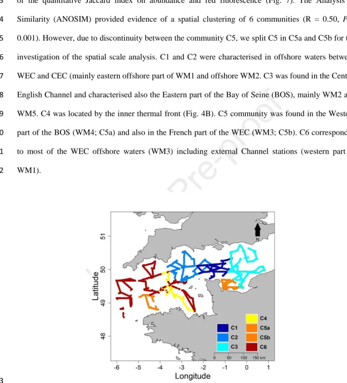
371
Phytoplankton communities were discriminated after the computation of a hierarchical classification 372
of the quantitative Jaccard index on abundance and red fluorescence (Fig. 7). The Analysis of 373
Similarity (ANOSIM) provided evidence of a spatial clustering of 6 communities (R = 0.50, P = 374
0.001). However, due to discontinuity between the community C5, we split C5 in C5a and C5b for the 375
investigation of the spatial scale analysis. C1 and C2 were characterised in offshore waters between 376
WEC and CEC (mainly eastern offshore part of WM1 and offshore WM2. C3 was found in the Central 377
English Channel and characterised also the Eastern part of the Bay of Seine (BOS), mainly WM2 and 378
WM5. C4 was located by the inner thermal front (Fig. 4B). C5 community was found in the Western 379
part of the BOS (WM4; C5a) and also in the French part of the WEC (WM3; C5b). C6 corresponded 380
to most of the WEC offshore waters (WM3) including external Channel stations (western part of 381
WM1). 382
383
Figure 7: Phytoplankton communities based on the results of the fusion between Jaccard similarity 384
matrice on the abundance and red fluorescence. 385
Heterogeneity was supported by the values of the coefficient of variance (CV) calculated for each 386
group, in addition, to minimum, maximum of abundance and total red fluorescence (further details in 387
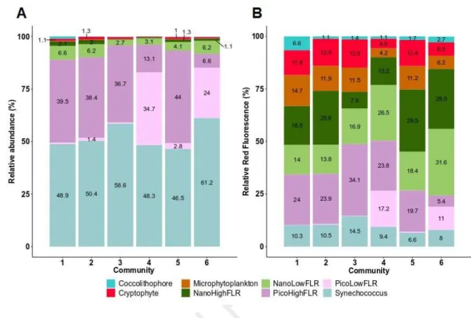
supplementary table A.1). In terms of abundance (Fig. 8), phytoplankton communities were all 388
dominated by the Synechococcus-like group (47% in C5 to 61% in C6 to the total abundance). 389
Picoeukaryotes (i.e. PicoLowFLR and PicoHighFLR) groups represented the second most important 390
groups (Fig. 8). However, in C1, C2, C3 and C5, the PicoLowFLR (36% in C3 to 43% in C5) 391
dominated over the PicoHighFLR (1% in C1, C2 and C3 to 3% in C5) whereas in C4 and C6, the 392
PicoHighFLR (24% and 34% respectively in C4 and C6) dominated over the PicoLowFLR (7% and 393
13% respectively in C6 and C4). On the other hand, the total abundance of nanoeukaryotes was always 394
low (at most they represented 11% of the total abundance for C1). The most abundant nanoeukaryotes 395
group was NanoLowFLR (3% in C3 and C4 to 7% in C1). In C2, the Cryptophyte-like cells total 396
abundance was the double than in any other assemblages. The most important contribution of the 397
Coccolithophore-like cells was found in C1 (1%) whereas in the other communities they accounted for 398
less than 1%. Finally, the total abundance of the microphytoplankton in every community was below 399
1%. 400
Although small photoautotrophs significantly dominated abundance (Fig. 8) in both WEC and CEC 401
during the cruise, the contribution of nanoeukaryotes and microphytoplankton to total red 402
fluorescence, which is an estimation of chlorophyll a fluorescence (Haraguchi et al., 2017), was 403
important (supplementary table A.1, Fig. 8). The relative contribution of the Coccolithophore-like 404
cells to the total red fluorescence was almost seven times higher in C1 than in any other community. 405
On the other hand, nearly half of the total red fluorescence in C3 and C4 was attributed to 406
Synechococcus-like and picoeukaryotes groups (C3: 49% and C4: 50%). This was higher than in the 407
other communities (range between 25% in C6 to 34% in C1 and C2). In C1, C2, C3 and C5, 408
Cryptophyte-like cells total red fluorescence represented the double (12-13%) of what they 409
represented in C4 and C6 (respectively 5% and 6%). In C3, C4 and C6, NanoLowFLR contribution to 410
the total red fluorescence (respectively C3: 17%; C4: 27% and C6: 32%) was higher than the 411
contribution of the NanoHighFLR (C3: 8%; C4: 13% and C6: 29%). We noticed the opposite pattern 412
in C1, C2 and C5. Despite the low abundance of the microphytoplankton group, the contribution to 413
total red fluorescence of this group was comprised between 4% (C4) and 15% (C1). 414
415
416
Figure 8: Relative contribution of phytoplankton, A. abundance and B. total red fluorescence, within 417
each community. Only the percentage above 1% are displayed. 418
Although we observed an heterogeneity in total red fluorescence per cluster, the CytoSense provided 419
us with information on single-cell level features (Fig. 9). Therefore, working at the individual level led 420
us to study the population variability considering a cytometric-derived trait. Here, we first focused on 421
the red fluorescence per cell and then on the cell-size. Different spatial patterns of red fluorescence per 422
cell and cell size were observed, per group, among the communities. Synechococcus-like red 423
fluorescence per cell remained unchanged in all the communities despite changes in cell size and 424
abundance (Fig. 9 A and B). Cell size was significantly different between all the communities 425
identified (p<0.01). Both picoeukaryote groups (i.e. PicoLowFLR and PicoHighFLR) exhibited the 426
most important red fluorescence per cell in C4 and C6 than in the other communities (p<0.05). For the 427
PicoLowFLR, the community comparison showed a large range of abundance within an order of 428
magnitude of 102 cell mL-1 whereas red fluorescence level remained between 200and 400 a.u. cell-1 429
(Fig. 9A). An increase in the red fluorescence per cell was observed with an increase of the cell size 430
(Fig. 9B). On the contrary, for the PicoHighFLR, high red fluorescence levels were consistent with 431
low abundance (Fig. 9A) and different relation between red fluorescence and cell size were observed 432
(Fig. 9B). Small cell with high red fluorescence levels were found in C4 and C6. Small cell with low 433
red fluorescence were found in C1, C2 and C4 and large cell with some level of red fluorescence were 434
found in C3. Concerning Cryptophyte-like cells and Microphytoplankton groups, the highest red 435
fluorescence values per cell were found in C5 and C6 and were significant (p<0.05). In these 436
communities, the Cryptophyte-like cells exhibited also the highest abundance (Fig. 9A and B) and 437
their cell size was significantly larger in C4, C5 and C6 than in C1, C2 and C3 (p<0.05). 438
Coccolithophore-like cells showed higher red fluorescence per cell in C2, C4 and C6 than in C1, C3 439
and C5. Moreover, the highest values of red fluorescence per cell were observed for NanoLowFLR 440
and NanoHighFLR in C4, C5 and C6. Finally, larger cell size was recorded in C4, C5 and C6 than in 441
C1, C2 and C3 for PicoLowFLR, Coccolithophore-like cells, NanoLowFLR and NanoHighFLR, but 442
no pairwise assemblage was significantly different. The log-log relation between red fluorescence and 443
orange fluorescence, per cell, showed an increase in fluorescence emission with the cell size (Fig. 9B). 444
In addition, there was an increase in the red and orange fluorescence emission as the cell size increases 445
(Fig. 9D) despite the standard deviation showed large variation for the orange fluorescence. 446
For red fluorescence, three orders of magnitude were recorded from the smallest (Synechococcus-like 447
cells) to microphytoplankton cell size. Synechococcus-like and Cryptophyte-like cells could be 448
characterized by a higher orange over red ratio from the other groups. However, not all groups 449
subscribed to this relation. Indeed, the figure 10B showed that some groups exhibited a change in size 450
but not in red fluorescence per cell (range of the standard deviations). This occur in specific 451
communities or in each community. For example, PicoHighFLR exhibited a large range of cell size 452
and red fluorescence in C6 and C1 whereas the size and the red fluorescence were fluctuating 453
irrespective to each other in the rest of the communities. Such patterns were also observed for the 454
Coccolithophore-like cells. This relation would mean that in some case the red fluorescence per cell is 455
independent of the size of the cells. As chlorophyll a fluorescence reflects the endogenous 456
concentration of this pigment, the relation between red fluorescence per cell and cell size may result 457
different intracellular pigment composition (Álvarez et al., 2017). On the other hand, the other groups 458
(i.e. Synechococcus-like cells, PicoLowFLR, nanoeukaryotes, microphytoplankton and Cryptophyte-459
like cells) tended to show a balance between the size and the red fluorescence, the larger a cell was, 460
the more red fluorescence it would emit. Finally, the range of the standard deviation in red and/or 461
orange fluorescence emission showed that the emission of red fluorescence per cell within 462
PicoLowFLR, PicoHighFLR, NanoLowFLR, NanoHighFLR, Cryptophyte-like cells and 463
Coccolithophore-like cells groups were not proportional to the emission of orange fluorescence per 464
cell. On the contrary, the emission of red fluorescence per cell was proportional to the emission of 465
orange fluorescence per cell concerning Synechococcus-like cells and Microphytoplankton (Fig. 9D). 466
467
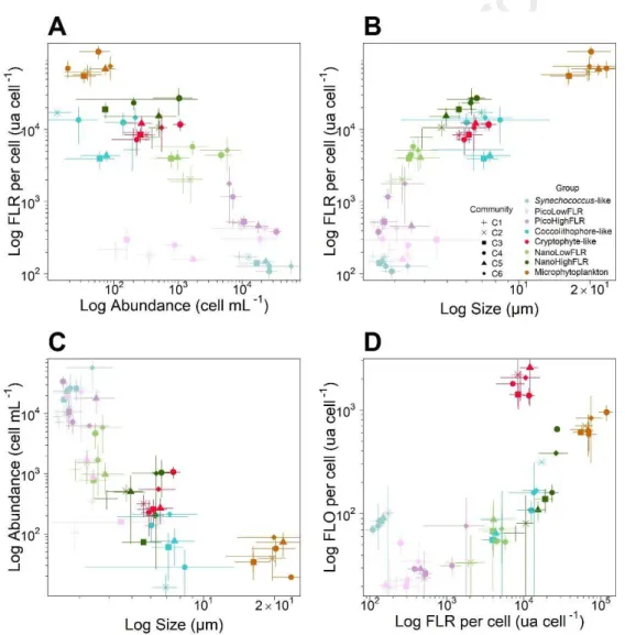
Figure 9: Patterns in size structure and fluorescence of phytoplankton groups amongst different 468
communities defined in the English Channel. A. Log-log relationship between phytoplankton 469
abundance and the red fluorescence per cell, per group and per community, B. Log-log relationship of 470
the red fluorescence per cell (FLR) against the phytoplankton size scaling per group and per 471
community, C. Log-log relationship between phytoplankton cell size and abundance per group and per 472
community, D. Log-log relationship of the orange fluorescence per cell (FLO) against the red 473
fluorescence per cell (FLR) per phytoplankton group and per community. 474
3.4 Variance partitioning
475
Results of the variance partitioning (pure spatial, pure environmental, interaction between environment 476
and space and unexplained variance) of the whole phytoplankton community and of each of the six 477
assemblages were summarized in table 2. Such analysis revealed that spatial (PCNM spatial 478
descriptors) and environmental variables (temperature, salinity and turbidity) accounted for 65% of the 479
total variance on the whole cruise. The 35% of the residual variance (i.e. unexplained variance) were 480
explained by other factors than environmental variables and space (e.g. biological processes such as 481
grazing, infection without interaction with the environmental data; Table 2). The spatial descriptors 482
(based on the spatial coordinates of sampling points) were more important than the environmental 483
variables (<5% for all the groups) in structuring the abundance and total red fluorescence of each 484
group. The spatial descriptors ranged between 24% (Coccolithophore-like cells) and 34%-36% (all the 485
other groups). The results were provided in the supplementary table A.2. Focusing on the 486
communities, the spatial variation of the assemblages was higher than the environmental variation 487
within C1, C2, C3, C5 and C6. In community C4, the environmental variation accounted for 45% and 488
was similar to the spatial variation which accounted for 43%. Then, the spatially structured 489
environment (i.e. interaction) accounted between 13% (C1) and 46% (C6) of the total variation. 490
Finally, considering the six communities identified (C5a and C5b are merged), both spatial and 491
environmental variables accounted for a significant amount of variation except for the effect of the 492
interaction between environment and space in C1. The sum of pure spatial, pure environmental 493
variables and their interaction explained from 40% (C1) to 74% (C6) of the total variation in the 494
communities. Therefore, the percentage of unexplained variation in the phytoplankton assemblages 495
was comprised between 26% (C6) and 60% (C1). 496
497
Table 2: Variation partitioning of phytoplankton community (Environment including temperature, 498
salinity and turbidity; space including abiotic interactions, physical processes and unexplained 499
environment). 500
Environment Space Interaction Residual
R² Adj. p-value R² Adj. p-value R² Adj. p-value
All 0.26 0.001 0.65 0.001 0.26 0.001 0.35 C1 0.15 0.001 0.25 0.001 0.13 0.06 0.60 C2 0.19 0.001 0.51 0.001 0.16 0.001 0.47 C3 0.59 0.001 0.60 0.001 0.43 0.001 0.34 C4 0.45 0.001 0.43 0.001 0.36 0.001 0.49 C5 0.35 0.001 0.44 0.001 0.27 0.001 0.48 C6 0.50 0.001 0.70 0.001 0.46 0.001 0.26 501
3.5 Scale of variability of phytoplankton communities
502
The multivariate Mantel correlogram based on the abundance and the average total red fluorescence 503
per cluster revealed phytoplankton communities’ spatial pattern by computing the geographical 504
distance between pairs of sites in each community (Fig. 10). The Mantel correlogram indicated the 505
highest autocorrelation at nearer distances, with a decrease and always reaching negative values at 506
farther distances (but not always at the same distance). Because C5 community was not spatially 507
continuous, C5 community was split into C5a (Eastern Bay of Seine) and C5b (South-Western of the 508
WEC) sub-groups. The highest autocorrelation was found in C4 and C5b (r=0.34 and r=0.40, 509
respectively). Phytoplankton assemblages showed a positive spatial autocorrelation between 20 km 510
(C5a) and 110 km (C6, Fig. 11). This meant that phytoplankton composition became more different 511
when the autocorrelation reached null or negative values. The definition of the spatial scale resulted in 512
the combination of high correlation for the nearer distances and the quick decrease of the correlation 513
when the distance increased. Here, the results suggested a high spatial structure at sub-mesoscale (<10 514
km) up to 110 km. This analysis confirmed the results of the partitioning variance analysis which 515
mentioned that space had a great influence in structuring the assemblages. 516
517
Figure 10: Mantel Correlogram of pairwise similarity in phytoplankton communities (Jaccardized 518
Czekanowski similarity based on the abundance and average total red fluorescence per cluster) against 519
geographical distance (Euclidean distance). 520 521 4. Discussion 522 4.1 Water masses 523
Despite the English Channel is a rather well-studied area, only few surveys attempted to characterise 524
the spatiotemporal distribution of physicochemical parameters in the CEC and WEC (Bentley et al., 525
1999; Charria et al., 2016; Garcia-Soto and Pingree, 2009; Napoléon et al., 2014, 2012). Most studies 526
benefited of long-term coastal monitoring or transect of ships-of-opportunity through a year. In the 527
present study, the focus was put in the whole Western and Central English Channel gridded at a 528
specific period of a year. Although the sampling strategies differed, our results showed similar 529
hydrological areas than previous studies. The water circulation from West to East in the English 530
Channel explained the longitudinal gradient observed during our study especially for the slow salinity 531
decrease (Salomon and Breton, 1993). In addition to this circulation, the vertical stability induced 532
during summer, contributed to the longitudinal gradient of temperature. Along the English coast of the 533
Central English Channel, the high values of turbidity were congruent with continuous run-off from the 534
Solent and were entertained in the gyre of the Southern part of the Isle of Wight (Ménesguen and 535
Gohin, 2006). During the CAMANOC cruise, strong horizontal gradients of temperature, salinity and 536
turbidity revealed five distinct water masses. The temperature gradient revealed tidal mixing fronts 537
where a strong stratification occurred (Simpson and Nunes, 1981). The stratification of the Ushant 538
frontal area (Garcia-Soto and Pingree, 2009; Pingree, 1980; Pingree et al., 1975; Pingree and Griffiths, 539
1978) separated 2 water masses (WM). WM3 corresponded to Western English Channel (WEC) 540
waters displaying mixed water column, lower temperature and higher salinity than the rest of the 541
waters of the outer Channel (shelf front) and the eastern WEC. WM3 was surrounded by stratified 542
waters. The western boundary corresponded to an external front separating warm and stratified waters 543
(Celtic Seas shelf waters) from mixed and cold waters (WM3). At the east, an internal front separated 544
cold and mixed waters (WM3) from warm and well-mixed waters (WM1). The temperature pattern 545
observed in the offshore waters was not consistent with observation in 2011 (Marrec et al., 2013; 546
Napoléon et al., 2013) but was congruent with negative anomaly observed in 2012 in the northern part 547
of the WEC (Marrec et al., 2014). We explained that by a combination of a relatively higher stability 548
of water in WM3 (low tidal stream) than in the CEC (high tidal stream) and the lower temperature 549
which are supported by air-sea heat fluxes shifting from positive to negative balance during the 550
summer-autumn transition. Thus, the upper mixed layer deepens and water cools down (Hoch and 551
Garreau, 1998). WM1 was characterized by high stable temperature and salinity (Fig. 4B). It might 552
have corresponded to the external front separating the WEC and the Celtic Seas in the Western border 553
and the internal front between the WEC and the CEC in the Eastern border. A latitudinal salinity 554
gradient revealed a salinity front separating WM4 found in the Bay of Seine (BOS) from the CEC 555
waters (WM2). The turbidity gradient separated the offshore waters of the CEC from English coastal 556
waters of Central English Channel (WM5). The low values of N² in WM4 (BOS) resulted from 557
permanently mixed waters even under the influence of the run-off of the Seine River (Bay of Seine; 558
French coast) whereas WM5 might have been under the remote influence of the Solent (English 559
Coast), leading to a slight dilution of coastal waters (compared to lower salinities recorded in the Bay 560
of Seine). WM2 could result in intermittently stratified waters (Van Leeuwen et al., 2015) in the 561
continuity of WEC stratified waters. 562
4.2 Phytoplankton communities
563
Several studies attempted to numerate phytoplankton assemblages in the whole area of the WEC and 564
CEC but none of them with high spatial (Garcia-Soto and Pingree, 2009; Napoléon et al., 2014, 2013, 565
2012) expanded gridding of data or on high temporal resolution (Edwards et al., 2001). Furthermore, 566
in this area, while previous studies focused only on species of the large size fraction of the 567
phytoplankton (i.e. microphytoplankton; Napoléon et al., 2014, 2012; Smyth et al., 2010; Tarran and 568
Bruun, 2015; Widdicombe et al., 2010), we were able to detect the whole size-range of phytoplankton 569
from picophytoplankton (1 µm) to large microphytoplankton (several millimeters length) in a single 570
analysis. Even though we did not reach a taxonomical resolution, it was possible to address the fine 571
structure of phytoplankton functional groups, as well as some of their traits, during the summer-572
autumn transition. 573
In this study, we used the CytoSense parameters derived from the optical features and signatures as 574
cytometric-derived traits at the individual and populational level (Violle et al., 2007) while several 575
studies were applying the same technique and approach in different aquatic ecosystems focusing only 576
one level (Fragoso et al., 2019; Malkassian et al., 2011; Pomati et al., 2011; Pomati and Nizzetto, 577
2013). The four selected traits (abundance per group, orange and red fluorescence per cell and cell 578
size) showed a spatial heterogeneity for each group, between the communities (Litchman et al., 2010). 579
The cell size was independent of cell’s physiology per group between our communities (larger cells 580
and higher average red fluorescence per cell in the community of the WEC, C4 and C6 than in the 581
communities of CEC and BOS, C1, C2, C3 and C5). This result suggests specific responses of the 582
species and/or groups. Indeed, in order to explain the spatial heterogeneity of the traits, we propose 583
three hypothesis: (i) the selection of the optimal traits under biological pressures such as grazing 584
(Litchman et al., 2009); (ii) the plasticity and genetic adaptation of the traits derived from the gene 585
expression in response to environmental variations (Litchman et al., 2010) and; (iii) in the case of the 586
automated “pulse shape” flow cytometry, a group can pool several species with similar optical 587
properties (Thyssen et al., 2008a). Here, as grazers were not recorded continuously, we decided not to 588
discuss about this hypothesis but would rather investigate the two others. 589
First, we suggest that the main drivers of the spatial variations are the temperature and the vertical 590
stability of water masses. The results showed that PicoLowFLR group, Cryptophyte-like cells, 591
nanoeukaryotes and microphytoplankton of the communities characterizing stratified and warm waters 592
(C4) and mixed and cold waters (C6) exhibited the largest average cells size and the highest red and 593
orange fluorescence per cell. Because the optimum for growth range of both nanoeukaryotes and 594
microphytoplankton is relatively low, the colder temperatures measured in WM3, characterized mainly 595
by C6, might have contributed to enhance their metabolism, hence, their size (Marañón, 2015). On the 596
contrary, despite small phytoplankton (picophytoplankton) are dominant everywhere at this period, 597
their growth is facilitated in water masses exhibiting high temperature values (C1 to C5, all WM 598
except WM3). Indeed, their temperature optimum for growth range is higher than nanophytoplankton 599
and microphytoplankton optimum growth range and should favor them in those conditions. Thus, in 600
water masses exhibiting cold water, we expect a dominance of larger cell size whereas in warmer 601
waters a dominance of the smaller cell size within a group. Although, nutrient and grazing rate were 602
not available at the same spatiotemporal resolution as the biological data, we are aware that both play 603
a role on cell size as well as their physiology. In the first case, the growth of small cells (i.e. 604
Synechococcus-like cells and picoeukaryotes) is favored against large cells (i.e. microphytoplankton) 605
under low nutrient condition (usually from the end of the spring bloom to fall). Then, biological 606
interactions (grazing, parasitism) are usually to impact cell size (Bergquist et al., 1985; Marañón, 607
2015) and physiology (Litchman, 2007; Litchman et al., 2010; Litchman and Klausmeier, 2008). 608
Finally, size overestimation of Synechococcus-like cells and picoeukaryote (Fig. 9) results of technical 609
drawbacks of flow cytometry. It is attributed to the halo effect of the laser which increased as particle 610
were increasingly smaller than the width of the laser beam (i.e. 5µm). 611
The heterogeneity of environmental conditions within a water mass affect the expression of the traits 612
within each group. For example, the Coccolithophorids are known to prefer warm and stable waters 613
(WM1) for their growth. Here, the PSFCM detected high total abundance of this group in the Celtic 614
Seas shelf, out of the English Channel (WM1, Fig. 5 and 6) which are dominated in this range of 615
abundance by Emilinia huxleyi (Garcia-soto et al., 1995). On the contrary, microphytoplankton 616
(including some diatoms and dinoflagellates) are known to grow and exhibit higher size in cold 617
waters, turbulent system, rich in nutrient. This explanation is also true for the nanoeukaryotes (i.e. 618
NanoLowFLR and NanoHighFLR). This is congruent with the WM3 and WM4 being influenced by 619
the Seine river (C5) and both by the Atlantic Ocean waters and the Seine River (C3). They both 620
contribute to provide nutrients. In addition, the low vertical water stability observed in the coastal 621
communities (along the French coast of Brittany, Bay of Seine) could increase small-scale turbulence 622
which might be positive for some groups (microphytoplankton, Cryptophytes-like, nanoeukaryotes) by 623
increasing nutrient transport (Karp-Boss et al., 1996). 624
On the other hand, all the groups exhibited different levels of red and orange fluorescence per cell 625
between the communities, except Synechococcus-like cells which showed the same levels across the 626
communities (Fig. 9A, B and D). The fluorescence emission given by each group is dependent on the 627
physiological states of the cells. The quantum yield of the chlorophyll a fluorescence (i.e. red 628
fluorescence of the PSFCM) and phycobilin and phycoerythrin (i.e. orange fluorescence of the 629
PSFCM) is also dependent to the life cycle of the cells leading to high fluorescence for young and 630
efficient cells whereas lysis is decreasing the fluorescence emission. Another point was linked to the 631
atmospheric conditions during the cruise. At the beginning of the cruise (corresponding mainly to 632
communities C6, C5 and C4 in WEC waters), the weather was sunny and without wind, some groups 633
(picoeukaryotes, nanoeukaryotes and microphytoplankton) showed high variability in orange 634
fluorescence per cell within a single community. The strong light intensity and the high stability might 635
have resulted in the synthesis of photoprotective pigments. However, the change of weather after half 636
of the cruise (while investigating WM3 and C1) might have enhanced the vertical mixing. Therefore, 637
the position of phytoplankton cells of the groups is permanently engendered by the mixing of the 638
water column which do not the induce production of photoprotective pigments. 639
Finally, the last case concerns the lack of taxonomical resolution of the automated “pulse shape-640
recording” flow cytometer. Indeed, our number of groups was limited. By sharing similar optical 641
properties, several species are attributed to a same cluster. In WEC waters, flow cytometry surveys 642
showed that picophytoplankton is usually composed of Prasinophyceae and usually dominated by 643
Ostreococcus sp. at this period of the year (which are considered as red picoeucaryotes by flow 644
cytometry). In addition, among the cryptophytes, few genera exhibiting a wide size range (between 5 645
and 19µm) are commonly detected (Marie et al., 2010). Nanoeukaryotes are frequently represented by 646
Haptophytes, Stramenopiles and Chlorophytes. Emiliania huxleyi is always reported as the dominant 647
coccolithophore species and is known to bloom in the outer shelf of the WEC (Garcia-soto et al., 648
1995). In addition, a high diversity of diatoms and dinoflagellates is also observed in the WEC (e.g. 649
Widdicombe et al., 2010). Such taxonomical diversity results also in size diversity which is related to 650
physiological traits (Litchman et al., 2010). Consequently, the pigment expression varies. Here, the 651
variations of the trait’s expression considering the three hypotheses (the plasticity and genetic 652
adaptation of the traits, the selection of the optimal traits under biological pressures and the lack of 653
taxonomical determination by automated “pulse shape-recording” flow cytometry) lead to changes in 654
related traits such as nutrient uptake, cell carbon and nitrogen content within each groups and between 655
the communities. The fact that traits such as the cell-size, abundance and total or per cell red 656
fluorescence per group differed significantly between communities, suggests optimum growth 657
conditions in the recorded abiotic parameters for their growth combined with trade-off in biological 658
pressure and variations of the taxonomical composition. 659
4.3 Environment vs. spatial variations