Uncertainty component estimates in transient climate projections.

Its main contri- butions are (i) to demonstrate a methodology to investigate the full causal chain from global climate change to local economic flood losses; (ii) to show that

From each study, the fraction of eggs that were marked, settler sample size, number of marked settlers observed in the sample and any information available on exhaustivity of adult

Abstract: We investigate the economic impact of stochastic endogenous extreme events and insurance in a growth model. Our analytical results and computational experiments show that

Its main contri- butions are (i) to demonstrate a methodology to investigate the full causal chain from global climate change to local economic flood losses; (ii) to show that

Our assumption follows from the argu- ment that the position-valence nature of a conflict will be the primary characteristic of the substance; political decision makers will

For example, one model states that environmental input goes to sen- sors (vision, auditory, ...), then to short-term temporary working memory, and depending on what happens there,

Dupain, Estimates for the Bergman and Szegö projections for pseudo-convex domains of finite type with locally diagonalizable Levi form, Publications Mathemàtiques 50 (2006),

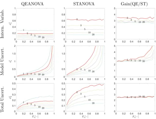
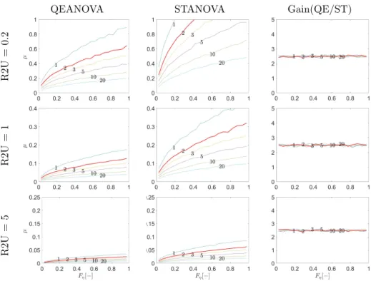
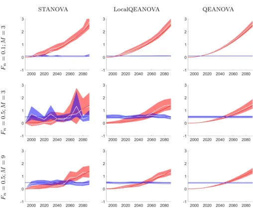
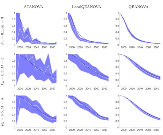
– SM2 : Large Scale and Small Scale Components of Internal Variability – SM3 : Comparing the precision of estimates in the Time Series ANOVA?. and the Single Time ANOVA approaches –