HAL Id: hal-00526345
https://hal.archives-ouvertes.fr/hal-00526345
Submitted on 14 Oct 2010
HAL is a multi-disciplinary open access
archive for the deposit and dissemination of
sci-entific research documents, whether they are
pub-lished or not. The documents may come from
teaching and research institutions in France or
abroad, or from public or private research centers.
L’archive ouverte pluridisciplinaire HAL, est
destinée au dépôt et à la diffusion de documents
scientifiques de niveau recherche, publiés ou non,
émanant des établissements d’enseignement et de
recherche français ou étrangers, des laboratoires
publics ou privés.
Parameter estimation for a marked point process within
a framework of multidimensional shape extraction from
remote sensing images
Saima Ben Hadj, Florent Chatelain, Xavier Descombes, Josiane Zerubia
To cite this version:
Saima Ben Hadj, Florent Chatelain, Xavier Descombes, Josiane Zerubia. Parameter estimation for a
marked point process within a framework of multidimensional shape extraction from remote sensing
images. ISPRS Technical Commission III Symposium on Photogrammetry Computer Vision and
Image Analysis (PCV 2010), Sep 2010, Paris, France. pp.1. �hal-00526345�
PARAMETER ESTIMATION FOR A MARKED POINT PROCESS WITHIN A
FRAMEWORK OF MULTIDIMENSIONAL SHAPE EXTRACTION FROM REMOTE
SENSING IMAGES
Saima Ben Hadj, Florent Chatelain, Xavier Descombes and Josiane Zerubia Ariana Research Group CNRS/INRIA/UNSA
2004, route des Lucioles - BP 93 - 06902 Sophia Antipolis Cedex - FRANCE
[email protected], [email protected], [email protected], [email protected] http ://www.inria.fr/ariana
Commission III, WG III/4
KEY WORDS: shape extraction, marked point process, RJMCMC, simulated annealing, SEM.
ABSTRACT:
Previously, an estimation method based on the Stochastic Expectation-Maximization algorithm was studied and proved its relevance for estimating the parameters of a marked point process model in order to achieve unsupervised feature extraction from remote sensing images. This method was only applied to a simple model of a marked point process of circles. In this paper, we extend the proposed estimation method to multidimensional shapes such as ellipses and rectangles. Different types of objects have been extracted: flamingos, tree crowns, boats, and building footprints. Furthermore, some prior constraints corresponding to the alignment of boats as well as the alignment of buildings are introduced.
1 INTRODUCTION
The problem of feature extraction from remote sensing images has been addressed in several scopes, namely, environment, civil-ian and military. As the resolution of the provided aerial and satellite images is very high, a smart technique of analysis of such data needs to be developed. In this context, a model of marked point process (Geyer and Møller, 1994, Møller and Waagepetersen, 2004) was previously introduced and proved its suitability to such a problem. It is basically a stochastic model that involves some information about the geometry of the objects present in the im-age. Certain parameters incorporated in this model must be ad-justed automatically, according to the processed image. In this prospect, a study of estimation methods of these parameters proved that a method based on the Stochastic Expectation-Maximization (SEM) algorithm (Celeux et al., 1996) was very relevant. It was firstly validated on a marked point process of circles (Chatelain et al., 2009a, Chatelain et al., 2009b). The aim of this paper is thus to extend this estimation procedure to more general geometrical shapes such as ellipses and rectangles. Several applications will be addressed, namely pink flamingo detection, tree crown extrac-tion, boat detection as well as building outline extraction. The paper is organized as follows: in the second section, we propose to review the family of marked point processes which has been used to extract surface networks. We then explicit the parameters of our model and describe the proposed estimation method. In the third section, we present the model of an ellipse process. Different tests using the associated estimation proce-dure have been performed. We discuss the obtained results and we modify the energy model spatially for boat detection. In fact, boats in a seaport are very close and aligned, which makes their discrimination difficult using the model proposed in (Chatelain et al., 2009b). In the following section, we look for the extraction of building outlines which can be represented by a network of rectangles. We therefore expose the adopted rectangle process. Moreover, we propose to append an energy component favor-ing aligned frames owfavor-ing that buildfavor-ings of large cities are usu-ally very organized. Finusu-ally we conclude this work by proposing some perspectives.
2 PROPOSED MODEL FOR OBJECT EXTRACTION AND PARAMETER ESTIMATION
2.1 Proposed model for object extraction
In a marked point process framework (Møller and Waagepetersen, 2004), image features are viewed as a set of objects identified jointly by their position in the image and their geometrical char-acteristics. Let W = P × M be the object space. Typically W is a bounded set of Rd, where P is the space of the object position
while M is the space of marks describing the object geometry. A configuration x of objects belonging to W is an unordered set of objects x = {x1, ..., xn} ∈ Ωn, xi ∈ W, i = 1, ..., n. A
point process X living in W is a random variable whose realiza-tions are random configurarealiza-tions of objects in Ω = ∪
nΩn. In our
work, we focus on a particular family of marked point processes, namely the familly of Gibbs processes. One major interest of these processes consists in their ability to model the interactions between objects. Denoting by y the observed image, the density of the considered marked point process is actually:
fθ(X = x|y) = e −Uθ(x,y)
c(θ|y) (1)
where c(θ|y) is the normalizing function written in the following formRΩe−Uθ(x,y)µ(dx) (where µ(.) is the intensity measure of
the reference Poisson process). θ is a parameter vector, allowing the flexibility of our model and its suitability to several types of images. It hence must be adjusted according to the given image. The process energy Uθ(x, y) is divided into the two types of
en-ergies: the external energy, Ud
θ(x, y) which quantifies the fit
be-tween the configuration x and the data y and the internal energy,
Up
θ(x) which reflects our prior knowledge about the interactions
between objects. Thus, the most likely configuration which al-lows object extraction corresponds to the global minimum of the total energy:
ˆ
x = arg max
x∈Ωfθ(X = x|y) = arg minx∈Ω[U d
θ(x, y) + Uθp(x)]
Algorithmically, the computation of the global minimum of this energy is performed by a simulated annealing scheme (Azencott, 1992).
2.1.1 Data energy Two main approaches for computing the data energy term were previously introduced to extract surface networks (Chatelain et al., 2009a). The first one was carried out in a Bayesian framework. Nevertheless, it doesn’t sufficiently take into account the morphology of objects. The second one is more efficient. It consists in defining a local energy Ud
θ(u) ∈
[−1, 1] associated with each object u. Then, the data energy as-sociated with a configuration x is proportional to the sum of all the local energies computed on each object u of x:
Ud θ(x, y) = γd X u∈x Ud θ(u, y) (3)
where the parameter γd > 0 corresponds to the data energy
weight. Its definition relies on a contrast measure between the distribution of the set of pixels belonging to an object u and the distribution of pixels belonging to its border Fρ(u). The data
en-ergy Ud
θ(u) is built as a qualification of this contrast measure in
order to promote well-placed objects and penalize bad ones:
Uθd(u) = Q(
d(u, Fρ(u))
d0 ) (4)
where d(u, Fρ(u)) is the Bhattacharya distance between the
ob-ject u and its boundary Fρ(u). Q
d0: R
+7→ [−1, 1] is a quality
function. It attributes a negative value to objects that have a high radiometric distance w.r.t. their border (i.e. d(u, Fρ(u)) is above
the threshold d0) and a positive value otherwise: Q(x) = 1 − x1/3 if x < 1, exp(−x − 1 3 ) − 1 if x ≥ 1. (5) Using a cubic root in this quality function ensures a moderate pe-nalization when the distance d(u, Fρ(u)) is close to the threshold
d0. To illustrate the behavior of such a function, we give its plot in figure 2(left).
2.1.2 Prior energy This energy corresponds to a penalization of the overlapping objects and thus avoids detecting the same ob-ject several times. For this purpose, we define the neighborhood system corresponding to overlapping objects by the following re-lationship:
∀xi, xj∈ W, xi∼ xj⇐⇒ Area(xi∩ xj)
min(Area(xi), Area(xj)) < s
(6) The parameter s ∈ [0, 1] represents the maximum recovery ratio between two objects. Afterwards, we introduce a “Hard Core” process which penalizes any configuration having at least one overlapping object pair with a recovery rate exceeding a thresh-old s. The non-normalized density of such a process is written as follows: hβ,γ(x) = βn(x)e−Us(x) where β is the activity
parameter, n(x) is the number of objects in the configuration x and Us(x) =
P
1<i<j<n(x)
ts(xi, xj) is the interaction potential
of objects in x. The interaction function between object pairs
ts(xi, xj) can be written as follows:
ts(xi, xj) =
(
0 if xi∼ xj,
+∞ otherwise. (7) By assigning an infinite energy to object pair that does not interact according to ∼, the associated probability is practically zero.
2.2 Estimation algorithm
Before revealing the proposed estimation method, it is necessary to identify the parameters to be estimated. The parameter vec-tor θ embedded in the considered model is composed of: the activity parameter β, the maximal overlapping ratio s, the data energy weight γd, the threshold d0involved in the quality
func-tion and the width of the boundary of an object ρ. Some of these parameters can be set in a deterministic way as they have an in-tuitive interpretation: The boundary width ρ is usually set to 1 or 2, the threshold s is set as the tolerated recovery proportion be-tween objects. The previous study of the model parameters has shown that the activity parameter β and the weight parameter γd
are correlated. The experience proved that a low value of β is compensated by a high value of γd and vice versa. Therefore,
we decide to estimate only one parameter which is the weight γd
and set manually the other ones. The problem of parameter esti-mation consists in identifying the most likely parameter vector θ that maximizes the image likelihood fθ(y). As the density of the
observation fθ(y) is unknown, we propose to maximize the
ex-tended likelihood fθ(x, y). However, the configuration x is
like-wise unknown. The study of estimation methods (Chatelain et al., 2009a) showed that the stochastic version of the Expectation-Maximization (SEM) algorithm (Celeux et al., 1996) is very rele-vant in such a situation. It consists in iterating the three following steps:
1. S step: Simulate a configuration of objects:
x(k)∼ f
θk(X/y) (8)
2. E Step: Evaluate the extended log-likelihood:
Q(θ, θk; y) = log fθ(x(k), y) (9)
3. M step: Maximize the log-likelihood:
θk+1= arg max
θ∈Θ Q(θ, θ k
; y) (10) Nevertheless, the E step is unreachable as the extended density
fθ(x(k), y) is not tractable (the normalizing constant is
inacces-sible). To overcome this difficulty, we propose to approximate the extended likelihood by the pseudo-likelihood (Besag, 1975, Bad-deley and Turner, 2000). Its expression in the case of incomplete data is given by:
P LW(θ; x, y) = exp µ − Z W λθ(u; x, y)Λ(du) ¶ × Y xi∈x λθ(xi; x, y) (11)
where λθis the extended Papangelou intensity which can be
writ-ten as follows: λθ(u; x, y) = β exp −γdUd(u) − X xi∈x/xi6=u ts(u, xi) (12) In practice, the simulation step is performed using a Reversible Jump Metropolis-Hastings algorithm (Green, 1995) or a multiple births and deaths algorithm. Afterwards, the maximization step is performed using the Nelder-Mead Simplex algorithm. The SEM algorithm is supposed to converge when the parameter vector re-mains stable. Once the parameters are estimated, we determine the most likely object configuration that maximizes the energy model thanks to a simulated annealing algorithm.
3 ELLIPSE MODEL 3.1 From circles to ellipses
Firstly, the estimation method was validated for a simple model of marked point process where the objects were circular (Chatelain et al., 2009b). Only one object mark corresponding to the radius of circles was introduced. The simulation results of the proposed approach on a 274 × 269 image of a flamingo colony in Camar-gue in France were not quite satisfactory (see figure 1). One can
Figure 1: left: flamingo colony in Camargue, France c°Tour de
Valat, right: flamingo extraction using a circle model: 363 circles c
°INRIA (β = 1000, γd= 13.88, s = 0.3, d0= 1.33).
notice misdetections on figure 1(right). Thus, such a model does not deal very well with the problem of flamingo extraction. A model of an ellipse process may be more suitable to the flamingo shape. This process is defined on the following object space:
W = [0, Xmax]×[0, Ymax]×[amin, amax]×[bmin, bmax]×[0, π[
which corresponds to the parameterization space of an ellipse u defined by five variables u = (x, y, a, b, ω). amaxand amin
are the parameters that demarcate the space of the semi-major axis a, and bmax and bmin are the parameters corresponding
to the definition domain of the semi-minor axis b. The figure 2(right) illustrates such a parameterization. This makes the
esti-0 2 4 6 8 10 −1 −0.8 −0.6 −0.4 −0.2 0 0.2 0.4 0.6 0.8 1 x Q
Figure 2: left: quality function, right: ellipse parameterization. mation algorithm time consuming since the number of parameters is increased using the ellipse process.
3.2 Validation of the ellipse model
In order to validate the proposed estimation method associated with an ellipse process, we tested it on three types of images; the flamingo image considered in the former paragraph, an im-age of trees in Saone-et-Loire of 229 × 196 pixels (figure 4(left)) and an image of boats of 385 × 275 pixels (figure 5(top)). For each image, we outfaced a new object structure. We manually initialized some parameters. The activity parameter was set as an over-estimation of the number of objects in the image, β = 1000 for all the treated images. The maximum overlapping rate was set to s = 0.3. All our simulations were performed using a processor with 1.86 GHz frequency. The estimation algorithm appears to be computationally expensive. It lasted 12 min for the flamingo
image (see figure 1(left)), 25 min for the tree image (see figure 4(left)) and 1 h and 36 min for the boat image (see figure 5(top)). The set of ellipses obtained at the convergence of the SEM algo-rithm for the flamingo image is revealed by the figure 3(right). After estimating the data weight, objects are extracted thanks to a simulated annealing algorithm. The estimates as well as the con-figurations of ellipses corresponding to the flamingo extraction, tree crown extraction and ship detection are respectively depicted in figures 3(right), 4(right) and 5(bottom). These results show that the proposed approach is very relevant for flamingo and tree crown extraction but does not fit the problem of boat detection. Therefore, we suggest in the second paragraph to modify the pro-posed model for the boat image. Moreover, to assess the accuracy of our solution, we have manually generated the ground truth of the flamingo image: the red ellipses are those that are automat-ically generated; the black ones are those that are supposed to appear (7 false negatives), the crossed red ellipses correspond to those that are wrongly detected (4 false positives) and all the red ellipses which have a blue point in their midst are considered as correct. From these results we compute the f-measure which is 0.98 and thus we conclude that our solution is very accurate (re-mark that an error up to 5% is acceptable for ecologists). Be-sides, the given results are only for one run, the table 1 gives an idea about the computational time average of several runs, the estimate mean γdand the standard deviation E [γd].
Figure 3: left: simulation step of the SEM algorithm, right: flamingo extraction using an ellipse model 387 ellipses c°INRIA
(β = 1000, γd= 16.25, s = 0.3, d0 = 1.33)
Figure 4: left: plantation in Saone et Loire c°IFN, right: tree
crown extraction using an ellipse model: 598 ellipses c°INRIA,
(β = 1000, γd= 15.14, s = 0.2, d0 = 2).
Flamingo image Tree image Boat image Mean time 41 min 24 min 1h and 41 min
γd 17.87 14.85 38.62
E [γd] 2.5813 0.5469 0.5427
Table 1: Statistical results
3.3 Modification of the energy model for boat detection As the boats of the image 5(top) are very close, the border Fρ(u)
of an object u is not homogenous. That is why, we modify its def-inition and we consider that it corresponds to the two ends of the
circumscribed crown (figure 6(left)). The corresponding SEM al-gorithm led to the estimate γd= 11.9512. The extraction results
displayed in figure 7 are enhanced, compared to those of the fig-ure 5(bottom). However, some false-detections corresponding to not aligned ellipses remained. To avoid this problem, we propose to favor close and aligned ellipses. For this purpose, we define an alignment interaction ∼albetween two ellipses (figure 6(right))
as follows: e1∼al e2⇐⇒ dω(e1, e2) ≤ dωmax dα(e1, e2) ≤ dαmax dC(e1, e2) ≤ dCmax (13)
where dω(e1, e2) =| ω1−ω2| is the difference of the orientation
of ellipses e1and e2, and dα(e1, e2) =| α − (
ω1+ ω2
2 +
π
2) | is a measure that checks that the ellipses are not shifted. Finally,
dC(e1, e2) =| d(c1, c2) − (b1+ b2) |, where d(c1, c2) stands for
the Euclidian distance between the centers c1and c2of the two
ellipses e1and e2respectively. Then, we append a prior energy
that promotes two tangent ellipses as follows:
Ual(e1, e2) = δ(dC(e1, e2), dCmax) . $(dα(e1, e2), dαmax) if e1∼al e2, 0 otherwise. (14)
where $(x, xmax) is a reward function, previously introduced in
(Ortner et al., 2008) to favor aligned buildings:
$(x, xmax) = − 1 x2 max · 1 + x2 max 1 + x2 − 1 ¸ , ∀ x ≤ xmax (15)
It is negative, when the measure x is below the threshold xmax
and zero, if the measure x equals xmax. The weight δ is
de-pendent on the distance between ellipses. It equals 1, when the ellipses are too close and is close to zero, otherwise. Finally, the prior energy of a configuration x, which corresponds to the alignment constraint is the sum over all the object pairs of the
Figure 5: top: photograph of vessels in France c°CNES, bottom:
boat detection using an ellipse model 508 ellipses c°INRIA (β =
1000, γd= 38.65, s = 0.3, d0= 6).
Figure 6: left: new definition of the ellipse border, right: tangent ellipses
Figure 7: Extraction results with modification of the data term: 635 ellipses (β = 1000, γd= 11.95, s = 0.3, d0= 6). configuration x: Ualp(x) = γal X 1<i<j<n(x) Ual(ei, ej) (16)
The weight γalis likewise a parameter of our model and must be
estimated by the SEM algorithm. The experience showed that a value of γallower than γdleads to good results for boat detection.
In our simulations, the initial value γ0
alused in the SEM algorithm
for the parameter γalis set to γal0=γd0/3, where γd0is the initial
value for γd(see (Chatelain et al., 2009b) for more details on
the numerical evaluation of γ0
d). The estimation procedure
con-verges after 1 h and 38 min and provides the following estimates:
γd= 25.3426 and γal= 10.535. The extraction results depicted
in figure 8 show that the ellipses are better organized. However,
Figure 8: Extraction results with an alignment constraint be-tween ellipses: 715 ellipses (β = 1000, γd = 25.34, γal =
10.53, s = 0.3, d0= 6).
one can notice some false-detections standing for aligned ellipses that are placed on the same boat (the number of boats automati-cally estimated is 715 while the hand-counted number of boats is 570). Furthermore, introducing a repulsive energy that penalizes not aligned ellipses does not enhance boat extraction results and leads to several misdetections. Thus, in a similar way to (Perrin et al., 2005), we propose to promote aligned ellipses that have a particular orientation (which is denoted by ωN), since the ships of
the processed image have a common direction. Thus, we modify the expression of the energy related to the alignment interactions of an object e as follows: Ualω(e) = ( Ualp(x ∪ {e}) − Ualp(x) if | ωe− ωN |≤ dωmax 0 otherwise (17) In order to validate this idea, we empirically define the boat di-rection and we then simulate the SEM algorithm corresponding to such a model. The estimates γd= 27.56 and γal= 9.18
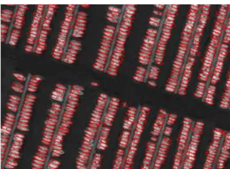
con-tribute to the detection of 523 boats depicted in figure 9. The
de-Figure 9: Extraction results favoring aligned ellipses having a particular direction: 523 ellipses (β = 1000, γd= 27.56, γal=
9.18, s = 0.3, d0= 6).
tection results are greatly improved. Nevertheless, this approach is not useful when the boats do not have a common direction. In this case, locally assessing the boat direction is a possible alter-native.
4 RECTANGLE MODEL 4.1 From ellipses to rectangles
In this section, we are interested in a marked point process which is defined in the following state space (a bounded set of R5):
W = P × M =[1, Xmax] × [1, Ymax] × [lmin, lmax]×
[Lmin, Lmax] × [0, π[
where (lmin, lmax) respectively stands for the minimum and the
maximum semi-width of the rectangle, (Lmin, Lmax) are the
minimum and the maximum of its semi-length and ω ∈ [0, π[ is its orientation. This parameterization is illustrated in figure 11(left).
4.2 Validation of the rectangle model
We simulate the estimation procedure associated with the de-scribed rectangle model on the Digital Elevation Model (DEM) of a part of Amiens image of 231 × 194 pixels, depicted on figure 10(left). Moreover, our tests were performed with the same CPU used in the previous simulations (a processor with 1.86 GHz fre-quency). The estimate γd = 29.402 contributes to the
config-uration displayed in figure 10(right), obtained at the extraction phase. Some rectangle pairs are not close enough and not very well aligned which could account for some misdetections. To overcome this problem, we propose to promote close and aligned rectangles.
4.3 Modification of the energy model for building outline detection
We propose to introduce an energy term that favors aligned and close frames. We thus use a similar component to that involved
in (Ortner et al., 2008). We define two different relationships be-tween building features; actually alignment and orthogonal inter-actions. In fact, orthogonal interaction is not viewed as a simple rotation between two interacted frames since some constraints on their appropriate edges must be taken into account as it will be explained later.
4.3.1 Alignment interaction We say that the rectangle u is aligned with the rectangle v, if one of its short edges is opposite to one short edge of the second rectangle v (figure 11(middle)). In other words, they are close enough such that the Euclidian distance dC(i, j) between the corner i of the rectangle u and the
corner j of the rectangle v is low and their appropriate short edges are opposite (i + j = 3) as well as they have almost the same orientation such that their angle difference (modulo π) dω(u, v)
is low enough: u ∼aliv, ∀i ∈ {0, 1, 2, 3} ⇐⇒ dC(i, j) ≤ dCm dω(u, v) ≤ dωm i + j = 3 (18)
Hence, the prior energy dealing with the alignment constraint is built such that it attributes a negative value to the pair of objects which exhibits jointly a low distance between their appropriate extremities and a low angle difference:
Uali(u, v) = 1 2$(dC(i, j), dCm) + 1 2 $(dω(u, v), dωm) if u ∼ali v 0 otherwise (19)
where $ (x, xmax) is a reward function given by equation (15).
Summing all the local energies over the object pairs of the figuration x, we actually obtain the alignment energy of the con-figuration x: Ual(x) = γal X 1<j<k<n(x) X 0≤i≤3 Uali(xj, xk) (20)
where γalis a regularization parameter that corresponds to the
alignment energy.
Figure 10: left: DEM of a part of Amiens c°IGN, right:
build-ing outline extraction usbuild-ing a rectangle model: 83 rectangles c
°INRIA, (β = 500, γd= 29.402, s = 0.2, d0= 4).
Figure 11: left: rectangle parameterization, middle: aligned rect-angles, right: orthogonal rectangles.
4.3.2 Orthogonal connection We propose to promote like-wise orthogonal frames. In fact, two rectangles are said orthogo-nal, if one rectangle short side is opposite to the other rectangle long side (figure 11(right)). That means, they satisfy the follow-ing conditions: u ∼orthiv, ∀i ∈ {0, 1, 2, 3} ⇐⇒ dC(i, j) ≤ dCm | dω(u, v) −π2 |≤ dωm i + j = 0, 2, 4 or 6 (21) By analogy with the expression (19) and (20), we define an en-ergy component of a configuration x, related to orthogonal con-nections ∼orthias follows:
Uorth(x) = γorth X 1<j<k<n(x) X 0≤i≤3 Uorthi(xj, xk)
where γorthis the weight of the described energy. Having
spec-ified the different types of connections that link buildings of an urban area, we can define an energy term that summarizes all the interactions between rectangles representing buildings as fol-lows: Up θint(x) = γint [U p al(x) + U p orth(x)] (22)
A new parameter γint related to rectangle interactions is
intro-duced in order to offset the value of the other parameters γaland
γorthwhich can be set to 1, since both alignment and
orthogo-nal connections are present in an equitable manner in the image 10(left). Hence, we are interested in estimating only one interac-tion parameter which is the weight γint, by the SEM algorithm.
Moreover, we initialize this interaction weight to γ0
int = γd0/2,
since the empirical test showed that it must have a lower value than that of the data energy weight γd. The SEM estimation
al-gorithm performed on the part of Amiens considered in the for-mer test is very slow. It required 6 h and 21 min and contributed to the following estimates γd = 30.0599 and γint = 16.8494.
The result of the extraction phase depicted in figure 12 shows that the frames are closer and more aligned than those of the previous simulation. However, some pairs are still distant. In fact, the
dis-Figure 12: Extraction results, favoring orthogonal and aligned rectangles: 83 rectangles (β = 1000, γd = 30.05, γint =
16.84, s = 0.3, d0= 4).
tance between two remote objects cannot support a new object without overlapping with them. To avoid such a case, we can in-crease the tolerated recovery rate s or we can employ object with variable size allowing the presence of small and large rectangles. In fact, in our tests we have limited the size of the occurred rect-angles when we have set the object space parameters.
5 CONCLUSION AND FUTURE WORK In this paper, we generalized the estimation method associated with a marked point process model to the case of multidimen-sional shapes such as ellipses and rectangles. The proposed es-timation method is based on the SEM algorithm. It showed its
interest for estimating the parameters of an ellipse process within the framework of flamingo and tree crown extraction. Its appli-cation to an image of boats in a seaport required the modifiappli-cation of both the data energy and the prior energy components of the proposed model. Moreover, in order to extract building footprint in a dense urban area, we introduced an energy term providing orthogonal and aligned frames. For that matter, we estimated by the SEM algorithm a new parameter related to this type of inter-action. Nevertheless, incorporating ellipse or rectangle process in an iterative algorithm such as SEM algorithm is time consuming. Accelerating the proposed algorithm by optimization strategies could be a nice future work. The computation of the pseudo-likelihood, representing more than 70% of the computation, could be parallelized using a multi-threaded program. Besides, the di-rection of boats involved in the prior term was set manually. It could be interesting to estimate it automatically.
ACKNOWLEDGEMENTS
The authors would like to thank the French Space Agency (CNES), the French Forest Inventory (IFN) and Tour du Valat for provid-ing the images presented in this paper. This research work has been partially supported by INRIA through a post-doctoral grant for the second author and partially by CNES through a contract.
REFERENCES
Azencott, R., 1992. Simulated annealing: Parallelization tech-niques. Wiley, NY, Springer-Verlag.
Baddeley, A. and Turner, R., 2000. Practical maximum pseudo-likelihood for spatial point patterns. Australian and New Zealand Journal of Statistics 42(3), pp. 283–322.
Besag, J., 1975. Statistical analysis of non-lattice data. The Statistician 24(3), pp. 179–195.
Celeux, G., Chauveau, D. and Diebolt, J., 1996. Stochastic ver-sions of the EM algorithm: An experimental study in the mixture case. Journal of Statistical Computation and Simulation 55(4), pp. 287–314.
Chatelain, F., Descombes, X. and Zerubia, J., 2009a. Esti-mation des param`etres de processus ponctuels marqu´es dans le cadre de l’extraction d’objets en imagerie de t´el´ed´etection. In: GRETSI’09, Dijon, France.
Chatelain, F., Descombes, X. and Zerubia, J., 2009b. Param-eter estimation for marked point processes. Application to ob-ject extraction from remote sensing images. In: EMMCVPR’09, Springer-Verlag, Berlin, Heidelberg, pp. 221–234.
Geyer, C. and Møller, J., 1994. Simulation procedures and likeli-hood inference for spatial point processes. Scandinavian Journal of Statistics 21(4), pp. 359–373.
Green, P., 1995. Reversible jump Markov chain Monte Carlo computation and Bayesian model determination. Biometrika 82(4), pp. 711–732.
Møller, J. and Waagepetersen, R., 2004. Statistical inference and simulation for spatial point processes. CRC Press.
Ortner, M., Descombes, X. and Zerubia, J., 2008. A marked point process of rectangles and segments for automatic analysis of Dig-ital Elevation Models. IEEE Transactions on Pattern Analysis and Machine Intelligence 30(1), pp. 105–119.
Perrin, G., Descombes, X. and Zerubia, J., 2005. A Marked Point Process Model for Tree Crown Extraction in Plantations. In: Proc. IEEE International Conference on Image Processing (ICIP), Genoa.