Estimating determinants of household water demand: evidence from urban and rural areas in Central Tunisia

HAL Id: hal-02606422

https://hal.inrae.fr/hal-02606422

HAL is a multi-disciplinary open access

archive for the deposit and dissemination of sci-entific research documents, whether they are pub-lished or not. The documents may come from teaching and research institutions in France or abroad, or from public or private research centers.

L’archive ouverte pluridisciplinaire HAL, est destinée au dépôt et à la diffusion de documents scientifiques de niveau recherche, publiés ou non, émanant des établissements d’enseignement et de recherche français ou étrangers, des laboratoires publics ou privés.

Marine Favre, Marielle Montginoul

To cite this version:

Marine Favre, Marielle Montginoul. Estimating determinants of household water demand: evidence from urban and rural areas in Central Tunisia. Journées de Microéconomie Appliquée, Jun 2016, Besançon, France. pp.26. �hal-02606422�

1

Estimating determinants of household water demand: evidence from urban and rural areas in Central Tunisia

Marine Favre, Marielle Montginoul

UMR G-Eau, Irstea, 361 rue JF Breton, BP5095, 34196 Montpellier cedex 5 – Tél : (33) 04 67 04 63 00 – marine.favre@irstea.fr

Working paper

Abstract

Knowledge of the determinants influencing domestic water demand constitutes an essential ingredient in the design of water policy in a context of increasing water scarcity due to climate and anthropic higher pressures. In this challenging environment, Tunisia is facing a current dual water supply, with households safely connected to water supply network and other poorly or not connected at all. Since the revolution of 2011, water access has become the core of the demand for an overall improvement in rural living conditions. Water demand has changed there, calling into question the current national balance in terms of resource and sector financing which will impact all the country because of current unbalanced water budget and the need to participate national effort to allow a safe access to all. Water demand has to be well known to better forecast needs, correctly design future water pricing system and other needy demand instruments in such a context of water scarcity. This study estimates water demand for piped and non-piped households using an original panel data at an individual level based on a survey conducted in 2014-2015. The price elasticity is estimated at -0.5 and -0.1 respectively for SONEDE-piped households and households piped to community systems’ networks. In non-piped rural areas, water demand seems to be essentially driven by variables characterizing the physical accessibility to water source.

Key words: demand estimation, household survey, household water demand, price elasticity, piped and non-piped water services, Tunisia

2 1. Introduction

Knowledge of the determinants influencing domestic water demand constitutes an essential ingredient in the design of water utilities’ policy in a context of increasing water scarcity due to climate change and anthropic higher pressures. When water demand is increasing and availability of water resources is not guaranteed or become too expensive due to technology required, water policy should encourage water demand management measures to prevent imbalance.

An important number of studies on domestic water demand have already been conducted in industrialized countries and some studies focus on the case of developing countries. As for now, empirical evidence from southern Mediterranean countries is still very scarce, especially from studies focusing on both urban and rural areas in a specific region. The main reason is that water may be unmetered and delivered by small suppliers who do not have a strict and centralized accounting system and which deliver water to only a limited number of households (Nauges & van den Berg 2009). To estimate water demand functions, household surveys are thus required which are highly complex to design because of the need to estimate water consumption.

This paper presents a case study focusing on central Tunisia comprising urban and rural areas. Since the revolution of 2011, water access (for domestic and also agricultural needs) has become the core of the demand for an overall improvement in rural living conditions (Gana 2012). In particular, water demand in rural areas has changed, calling into question the current national balance in terms of ressource and sector financing in Tunisia which will impact all the country. Households who are already connected to the national water supply network (SONEDE) will be especially impacted, because of current unbalanced water budget and the need to participate national effort to allow access to all.

The paper adds to the recent literature dealing with the issue of water demand in southern Mediterranean countries in the particular context of water scarcity. The first objective is to improve the knowledge of water demand determinants, both in urban and rural areas, by conducting an in-depth analysis at household level, contrary to previous works undertaken in Tunisia which focused on the regional district level solely in the urban sector (Ben Zaied 2013; Ayadi et al. 2002; Binet & Ben Zaïd 2011; Sebri 2013).

This improvement may be useful for general water sector planning and strategy design, as it documents the opportunity and the consequences of adding new connections while helping to estimate future water consumption and wastewater production, as soil and groundwater preservation is also becoming a crucial issue. Another specific objective is to estimate price elasticity in various contexts to anticipate responses to changes in water tariff structure and the design of tariff instruments in order to encourage water conservation.

3

This paper is organized as follows: after a presentation of the background, and a brief literature review, the methodology for data collection is explained. Then, the model specification is justified before presenting and discussing the results and, lastly, concluding.

2. Background 2.1. Water resource

In Tunisia, total renewable water resources per capita were estimated at 415 m³/inhabitant for 2014 and they could fall to 345 m³ in 2025 (Hamdane, 2007 quoted by Sebri 2013). The external dependence is low at national level as only 9.1% of national resources come from abroad (FAO Aquastat database for 2014). But territorial choices for the economic development of the country on coastal areas through tourism did not take into account the geographical imbalance of water resources (Touzi et al, 2010), leading to major transfer investments being made: coastal zones (Cap-Bon, Sahel, Sfax) have to derive 55% of their supply from regions of the north and north-west which transfer 74% of their production (SONEDE, 2008 quoted by Touzi et al, 2010). The Kairouan area is supplied from an aquifer renowned for its quality and which supplies other regions in Tunisia via large-scale transfer infrastructures.

2.2. Water access

In Tunisia, the national public operator SONEDE serves 100% of urban households and 50% rural households nationwide through individual connections (IC). In the other rural areas, water service is managed by water users’ associations (GDA1_{), supported by the Ministry of Agriculture (funding}

of initial infrastructure investment). Initially, with GDA systems, water is delivered through collective water kiosk. However, since the 2000s, and then exponentially after the 2011 revolution, a lot of households get their own IC from GDA’s network, sometimes legally within specific programs but most of the time illegally.

This article concerns a specific zone located in central Tunisia: the Governorate of Kairouan. In this governorate, 100% of urban households and 39% of rural households are supplied by SONEDE (through ICs), 50% of rural households are supplied by GDAs (16% by ICs and 34% by collective standpipes) and 10% are not supplied (SONEDE estimate in 2014). After the revolution, this governorate was particularly affected by illegal connections, boreholes and water theft in rural areas.

4 2.3. Water tariffs in the SONEDE area

SONEDE’s water tariff currently applied is uniform throughout the country. It is topped with a sewage collection and treatment charge, this service being operated by another national public operator, ONAS.

Water bills in urban areas and rural areas served by SONEDE include then one or two parts depending on the presence or not of sewerage. Water bills vary highly and by steps (Figure 1) both services having adopted binomial tariffs with increasing blocks.

Figure 1: Water bills (incl. VAT) paid quarterly by Tunisian households connected to SONEDE in tunisian dinars (TND2_{), in 2014, up to 200 m}3 _{quarterly consumption}

Concerning the water part (Figure 2 - left), SONEDE applies a fixed part depending on the diameter of the water meter. The variable part follows an increasing jump tariff structure: all consumption is charged at the rate of the last band. Beyond 40 m3, the water tariff grows fast with water consumption, this strongly incites consumers to save water.

Sewerage is priced in a different way (Figure 2 - right): the fixed part level depends on the water consumption level; the proportional part tariff structure is by increasing block tariff (IBT): the first cubic meters consumed are billed at a lower rate than the next one and so on, by blocks.

2 _{The exchange rate is EUR1=2.24 TDN as of 10/03/2016, it was EUR1=2.25 TDN at the time of the}

research (01/01/2015). 1114 24 38 59 91 129 150 223 292 0 50 100 150 200 250 300 350 400 0 20 40 60 80 100 120 140 160 180 200

Water bill including sewerage

Water bill without sewerage

m3 per quarter TND

5

Figure 2: Water and sewer rate structures paid by Tunisian households quarterly in Tunisian Dinars including VAT, in 2014, up to 200 m3 per quarterly consumption

As a consequence, marginal and average prices are strongly varying, as depicted in Figure 3. Marginal prices can then reach really high (and maybe not acceptable?) levels: from 2.773 DT to 65.184 DT, with the aim of topping consumption level. This jump tariff structure gives strong incentive to stay just under a block limit.

Figure 3: Average and marginal prices in TND including VAT, in 2014, up to 200m3 quarterly consumption

SONEDE has also been facing an increasing deficit since the early 2000s, because the level of the average price is not sufficient to cover its cost since 2004 (OCDE 2014). This is due to 2 factors: 1) Tariff increases have not been sufficient to offset the rise in inflation and 2) the tariff rates in lower bands don’t match with the consumption distribution curve to balance water budget: below the third band, tariffs cover only 50% of costs whereas about 70% of consumption is billed into those 2 first bands (Ben Mansour 2014).

Since the two price adjustments scheduled for SONEDE in 2007 and 2009 were not applied, SONEDE obtained in 2010 an agreement that prices would increase by 5% per year until 2016. The

0,183 0,319 0,431 0,785 0,962 1,339 5,19 0 1 2 3 4 5 6 7 8 9 10 0,0 0,2 0,4 0,6 0,8 1,0 1,2 1,4 0 20 40 60 80 100 120 140 160 180 200

Proportional part (TND / m3_{) Fixed part (TND)}

Fixed part (water)

Proportional part (water)

m3 _{per quarter} 0,648 0,321 0,321 0,524 0,505 0,193 0,3050,305 0,030 0,182 0,020 1,400 4,385 8,620 9,050 9,315 0 1 2 3 4 5 6 7 8 9 10 0,0 0,2 0,4 0,6 0,8 1,0 1,2 1,4 0 20 40 60 80 100 120 140 160 180 200

Proportional part (TND/ m3_{) Fixed part (TND)}

Fixed part (sewerage)

Proportional part (sewerage)

6

first increase took effect in 2010, but the reform was then interrupted by the revolution (Ben Mansour 2014). The price was once again risen in 2014 and over the past two years. If considering ONAS own tariff reform agenda (3 tariff reforms since 2013),water and sewer prices have increased frequently during the last years (Figure 4).

Figure 4: Evolution of water bill (including sewerage) between 2013 and 2015 per level of water consumption up to 200 m3 quarterly consumption – base 100 = 2013, January

2.4. Water tariffs in other rural areas

In rural zones supplied by GDAs, water price is not homogenous. GDAs therefore bill customers supplied by kiosks, and thus less conveniently, an average of TND3 _{0.2 to TND 1.2 per m}3 _{of water}

(personal communication, M. Mnajja Ministry of Agriculture, 2014 and observations in the field). When public access was privatized by illicit connections (Table 1), pricing per cubic meter was adopted, with a price ranging from TND 0.4 to TND 0.75.

Water access Price Locality

Individual connection (piped households)

0.400 TND/m3

0.500 TND/m3

0.750 TND/m3

Rmadhnyia

Nahala, Ruissat, Zbara Mtayria

Water kiosk 0.020-0.025 TND per 20 litres + transport charges (up to 20 TND)

Cheri-Chira, Ganzhour, Nahala, Rmadhniya, Ruissat

Tanker delivery 20 TND (3 m3₎

30 TND (5 m3₎

Nahala (suffering from long-run shortage)

Water container (20 or 40 litres) 1 TND Ruissat

Table 1: Type of access, price of water and place of access

3 _{The exchange rate is EUR1=2.24 TDN as of 10/03/2016, it was EUR1=2.25 TDN at the time of the}

7

Water price paid by non-piped users is even more variable, depending on the water access modes (Table 1): for a 20-litre container filled directly from a kiosk, the price is TND 0.020 while the same container delivered to the home is billed at TND 1. Tanker deliveries are also possible, leading to a price of about TND 6 per m3. These price lead often to bills higher than those paid by SONEDE customers.

3. Literature review

The literature on water demand modelling function is relatively extensive and has already given rise to several recent summaries including 3 meta-analyses (see Espey et al. 1997; Dalhuisen et al. 2003; Sebri 2014) and 6 literature reviews (Arbués et al. 2003; Baumann et al. 1998; Worthington & Hoffman 2008; Nauges & Whittington 2009; House-Peters & Chang 2011).

In industrialized countries, where drinking water supply through individual connections is almost generalized, the aim of determining factors explaining household water consumption is to help forecast future water consumption (planning) and to anticipate the reactions of the consumers when implementing demand management policies, in particular pricing reforms. The data used are most frequently derived from aggregate customer consumption data (for example for an entire municipality) provided by the water suppliers. At this level, however, as underlined by Nauges & Whittington (2009), some socio-economic information only available at the individual household level is not, by definition, incorporated. We are therefore dealing with systems which we assume provide a homogenous service in terms of price, water quality and service continuity and in which any variability in access to the water service is erased or at least averaged out.

In functional terms, the models usually take the form of the following classic single equation: q = f(p,x)

where q represents water consumption, p the price of water and x a vector of the household and accommodation characteristics.

The meta-analyses identify two common types of functional form adopted by studies: i) linear functions which do not provide a constant elasticity value at all points on the demand function and ii) log-linear functions with the advantage of providing a constant elasticity value for all points on the demand curve.

Espey et al. (1997) and Dalhuisen et al. (2003) find no significant difference between linear and log-linear forms while Sebri (2014) concludes that there is a significant difference, albeit small, between log-linear forms. Various regression forms are tested in the literature, but the three meta-analyses cited above highlight the absence of any significant difference between OLS estimators and other estimators (instrumental variables, fixed effects, random effects).

8

The factors most often identified as being significant are the water price, household income, climatic variables, household size and composition, the presence of non-tariff demand management instruments (Worthington & Hoffman 2008), the presence of household appliances (Nauges & Whittington 2009), accommodation characteristics and the different indoor and outdoor uses made of water (Arbués et al. 2003).

Particular attention is generally paid to the results of price and income elasticities, although the values are low ̶̶ often below 1 ̶̶ due to the fact that water is a non-substitutable good and that users have only a limited price perception when the bill represents a small share of income (Arbués et al. 2003). According to Espey et al. (1997), the average elasticity observed in 24 dedicated studies in the United States is -0.51 (90% between 0 and -0.75), while Arbués et al. (2003) note an income elasticity of between +0.1 and +0.4 in the studies they have reviewed for mostly industrialized countries and some developing countries.

One of the key questions in modelling the demand function relates to the specification of price when it is not simply volumetric but depends on the quantity consumed. This is the case, for example, with block tariff structures, binomial tariff structures with a fixed element and a variable element, and tariff structures which include free initial cubic meters. In these cases, the average price and the marginal price vary according to the quantity of water consumed, thereby leading to an immediate endogeneity between the variable to be explained and the explanatory price variable. To circumvent this endogeneity problem, several alternatives are put forward in the literature (Worthington & Hoffman 2008): the use of a difference variable or Nordin specification suggested by Nordin (1976); a two-stage model such as that proposed by Hewitt & Hanemann (1995), whereby a first discrete model explains the choice of a consumption block and then a second model explains the volume consumed by the household in the chosen block and the use of models with instrumental variables. Two other possibilities include adopting a price for a standard volume applied equally to all individuals (Montginoul et al. 2009) uses the average price for 120 m3 corresponding to a yearly average water consumption for a family), or using a lagged price variable which requires data over several periods. In contrast to Arbués et al. (2003), Sebri (2014) concludes that the price specification has a significant impact on the price elasticities recorded and it would even appear that differences in price specification affect the value of income elasticities.

In developing countries, there are fewer studies available on water demand. To the best of our knowledge, the state of the art proposed by Nauges & Whittington (2009) is the only recent analysis dedicated exclusively to studies conducted in developing countries. According to the authors, the use of (or the access to) numerous water sources by households is one of the characteristics of water provision in these countries. The difficulty in obtaining reliable and complete information for all the water systems available to the households would explain the smaller number of studies

9

conducted in this context. The socio-economic household survey appears then as one of the strategies to collect such data.

In countries where access modes are not homogenous and several types of supply may be available on a same location, it is important to control that certain household characteristics (observed or otherwise) are not correlated with the type of source and with the level of consumption - since water consumption level will then depend on the water access mode. Then a “source choice model” may be implemented to avoid a possible risk of sample selection bias in such a situation. Correlation between household characteristics and type of source may occur when the households have access to several sources and choose one specific sources as their main source or because by choosing their place of residence, it is deemed that households have chosen their water access mode (Larson et al, 2007) or even that the municipalities take the decision to supply a population with one or other system (public water kiosks, tanker truck for example) according to the household characteristics (as they can determine their capacity and willingness to pay, for example) (Nauges & Strand 2007). Once the source choice issue has been solved, the water demand function can be estimated. For households collecting water exclusively or primarily from one single source, studies usually estimate a water demand function per type of source or one equation per sub-group of households differentiated by their water access mode (Nauges & Whittington 2009). In the case where multiple sources are simultaneously used by households, several demand functions may be combined to measure substitutability and complementarity relations between the sources (see for instance Nauges & Strand 2007; Nauges & van den Berg 2009).

With regard to the water demand function, the same estimators are used as for industrialized countries (OLS, instrumental variables, fixed effects, random effects). The dependent variable is consumption per household or per inhabitant while the explanatory variables are water price, household characteristics (income, size, composition, family head profile), accommodation characteristics (size, type, garden, equipment, sanitary facilities), season, climate (rainfall, temperature) and water access (organization of fetching water, service continuity, water quality) Nauges & Whittington (2009).

4. Data

The data set used is original as it comes from a household survey we carried out in 2014-2015 in 16 localities in the north-west of the Governorate of Kairouan in Central Tunisia.

10 4.1. Methodology

Before starting the survey, targeted interviews conducted with institutional actors at national level (Ministry of Agriculture, SONEDE) and regional level (CRDA4_{, DR SONEDE) served to}

characterize the general water access situation at local level, to identify the different means of access to water and supply situations and to choose the locations (or sectors) to be surveyed.

At the same time, a draft questionnaire was tested with 20 urban and rural households. On the basis of the results of the first questionnaires and different discussions with the households and institutional actors, the questionnaire was adjusted and translated into Arabic.

Five students (two women and three men) from the region with at least two years’ higher education and bilingual in French and Arabic were recruited and trained. They were chosen on the basis of their comprehension of the questionnaire, the objectives, the method and their ease in the field. The survey introduced at each site was carried out in two stages. Initially, we visited each location after being announced by the SONEDE Regional Director or being accompanied by a CRDA’s civil servant in order to meet the local authorities and, where applicable, the local manager of SONEDE; we visited the sites, saw the supply systems and located the various accommodation districts. Subsequently, the entire team including the interviewers travelled to the locations to conduct the interviews. Each interview, lasting on average 20 to 40 minutes, was conducted one-to-one with an adult member of the household either at home or at the supply site. To ensure statistical representation of the observations while taking account of material constraints inherent to research (in particular logistical and budgetary, but also the workability of the sample to control the quality of the information collected), the decision was made to collect at least 30 questionnaires for each location (or per district in urban areas).

It was not possible to draw households at random using a table of numbers in each location for budget, time and logistical reasons (the dwellings are widely spread in rural areas) and the availability of the survey base. However, the households’ selection method tried to be close to the random sampling procedures: the interviewers were assigned to each district with the aim of conducting a minimum number of surveys per enumerator, determined according to the estimated population of each site, and were instructed to cover the site’s geography and not interview neighboring households. Three survey sessions were conducted in the locations between autumn 2014 and spring 2015.

4 _{The CRDA is a regional administration under the authority of Agriculture Ministry and who is in charge of}

11 4.2. Final sample

The 16 localities surveyed were selected according to the physical (drinking water distribution or irrigation network, no one, self-alimentation), institutional (SONEDE, GDA, un-served), and economic criteria of water access:

 8 locations supplied by SONEDE, 3 in urban areas, 1 in a peri-urban area and 4 in rural areas supplied for different durations (4 months, 2 years, 15 years, 25 years);

 7 rural locations supplied by GDAs with contrasting situations in terms of water resource (autonomous water source, SONEDE connection, purchase form another GDA), mode of water access (legal/illegal individual connection of the household or a neighbor, standpipes, water vendors, well), continuity of service (continuous supply, frequent interruptions, interruptions lasting several months or years);

 1 rural location unserved.

The sample size reached 655 households; 73% of the people interviewed were heads of household, 20% their spouse and 7% another adult within the household. Among the 655 households, 60% are located in urban or peri-urban areas and 40% in rural areas. In the SONEDE areas, 95% of households had an individual connection. In the other locations, 54% of households have a connection to a GDA network (functioning or non-functional at the time of the survey, either illicit or licit) and 46% have no connection. In the remainder of the present paper, these three sub-groups are named respectively SONEDE-piped households, GDA-piped households and non-piped households.

In 4 locations managed by GDA, the ICs installed are considered as illicit while in one location the ICs were installed under the control of the CRDA. Two locations benefit from a service which is occasionally intermittent but without long interruptions, one location suffers from an intermittent service which does not cover all the housing areas and two locations had had no water at the ICs for several months when the survey was conducted.

4.3. Questionnaire and additional data collection

The survey instrument (200 questions) consisted of several parts. The first section aimed at drawing a socio-economic profile of the households and described their living conditions. A second section identified the modes of water access, and evaluated the current level of consumption and associated costs. The third section determined the coping behaviors and strategies in the event of a service interruption or a change in the water access modes.

The main originality of the questionnaire lies in fact that we have endeavored to obtain a robust estimation of water consumption and its variability (between summer and winter, according to the water access mode for a single household, for example during an interruption), when water is not metered with an individual meter, the main difficulty encountered in these contexts (Nauges &

12

Whittington 2009). Only the SONEDE-piped households have meters which are read on a quarterly basis. For the latter, it was possible to obtain the information directly from SONEDE as the households communicated their customer number.

For GDA-piped households, no meter could be read (meter absent, hidden, illegible, removed). Consumption was estimated by comparing the following information collected from the households: i) an equivalent in litres per day they believe they consume, ii) volume consumed in the event of a shortage and the difference (as a number of containers) between usual consumption from the IC and the same consumption in the event of a shortage, iii) volume consumed before getting the IC and number of additional containers they think they now consume with the IC. It would appear that these questions worked well (high response rate) and provide similar values. Finally, with regard to non-piped households who are supplied via a source outside the house, the means of water supply was recorded per period and per type of access, and in particular the number of containers and the frequency with which they are filled were indicated by the households. The volumes declared can be considered as reliable for three reasons: i) access is often relatively far from the dwellings and households procure water a limited but regular number of times per period, ii) households have a limited number of empty containers and containers are expensive, iii) the number of containers and their capacity were summarized at least twice by enumerators through different questions asked during the interview.

Then the survey data were supplemented with daily meteorological data from the Weather Information Service provided by www.ogimet.com using specific data come from the NOAA system5 which relays the records of a station based in Kairouan city.

Finally, SONEDE billing records were collected for piped households on the 15 previous quarters (2012-2015), during which several tariff increases occurred. Households supplied by SONEDE are billed quarterly according to a meter reading timetable which differs from one zone to another due to the limited number of agents. Between two locations, the quarterly meter reading date can differ by up to two months, which means that the first quarter can run from January to March for one location but from March to May for another. The quarterly bills were divided into months so that they matched the calendar weather data.

5_{National Oceanic and Atmospheric and Administration published by United States Department of} Commerce.

13

5. Model specification and summary of main variables 5.1. Model specification

In developing countries, some authors note the need to control a possible selection bias when households choose their main source among several available sources (Nauges & van den Berg 2009) or when municipalities or authorities choose the type of access taking into account household characteristics (Nauges & Strand 2007). In our case, we consider that such a model is not applicable as the households are under too many constraints. First, households generally have access to a single source for their domestic consumption in the examined region (of course considering the main supply and not the periods of interruption when households are looking for alternative sources). The choice of which authorities should set up the infrastructures is then based on exclusively physical (availability of the resource), geographical (differences in altitude, distances) and land occupation (housing density) criteria.

In light of strong variations in consumption recorded between the two seasons (summer and winter), we choose to handle data as a panel in order to retain this seasonal dimension which can be useful both from an economic standpoint if we wish to introduce regulatory tools for demand (for example seasonal pricing) and from a technical standpoint to measure water needs.

For each household, we considered the reference season “summer” or “winter” to be the most recent past season. The panel data was created by pooling the observed responses for each household and the other data from OGIMET and billing records from SONEDE. With each of the two reference seasons “winter” and “summer” for each household, we matched the corresponding climatic variables and, only for households for which the bills were available, volumes invoiced for these two reference seasons. In light of the fact that not all households were interviewed during the same month (3 sessions spread over 1 year), not all households have the same two reference seasons. In the panel, certain variables vary with the individuals and time (consumption, price, climate), while others are invariable over time (socio-economic characteristics of the households and housing, means of access to water). Due to the missing data, the panel is unbalanced.

Household water demand was then estimated using random effects generalized least squares, for three reasons. First, the random effects model distinguishes itself from the fixed effects model by the fact that it considers that the individual specific effects are not deterministic but random. In our case, we work on survey data, a non-exhaustive sample drawn at random from a population, and it is preferable to consider that the individual effect is random and non-deterministic (Baltagi 2008). Then, our model combines an inter-variability (between) and an intra-variability (within) and thus satisfies the requirements of a random effects model which can be interpreted as a weighted average of the OLS model and the fixed effects model. In our case, the unobserved heterogeneities can be

14

of different dimensions: invariable over time and specific to each individual (cultural and religious practices, physical characteristics, etc.) which are sensitive variables to be included in surveys and difficult to estimate; variable over time but in a manner specific to each individual (exceptional use of other sources, creation of new temporary uses, temporary increase in the number of supplied people, etc.). Lastly, in more practical terms, this approach allows time-invariant household specific explanatory variables (such as income, household size) to be included in the demand equation since in the fixed effects model, these variables would have been absorbed by the intercept.

The basic form of the equation for the water demand function is as follows: Qis = α+ β X is + ɣ Z i + μ is

As a log-linear specification was retained, the equation takes the following form: Ln Qis = α+ βln X is + ɣ ln Z i + μ is

With Qis the log of the consumption of individual i in season s; α the intercept, ln X is the log of the

explanatory variables which vary in the two individual and seasonal dimensions, ln Z i the log of the

explanatory variables which do not vary in the single individual dimension; β and ɣ the vectors of the parameters we want to estimate and the error term μ covering two dimensions, individual and temporal (between-entity error and a within-entity error).

Considering water access modalities differ considerably between the three groups, we estimate three water demand functions separately for 1) SONEDE-piped households 2) GDA-piped households and 3) non-piped rural households using alternative access served by GDAs or unserved (kiosk, wells, water sellers). For the three equations, the variable to be explained is the quarterly consumption per inhabitant per season (3 months).

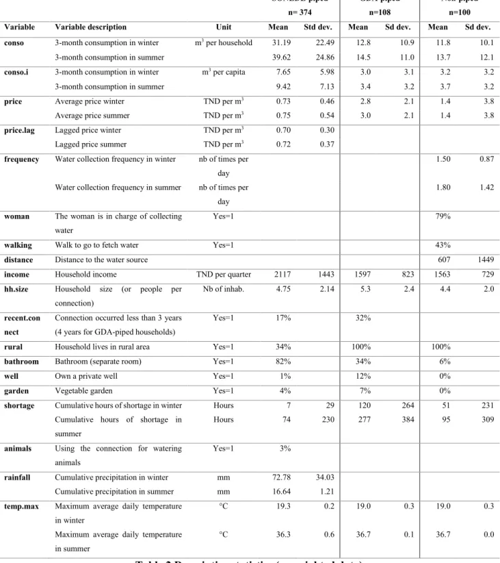
5.2. Description of variables and selected summary statistics

After data-cleaning, the usable sample size consisted of 582 households: 374 SONEDE-piped households, 108 GDA-piped households and 100 non-piped households. Some of the GDA-piped households and households living in the unserved locality were excluded from the analysis when consumption measurements are not deemed sufficiently reliable.

Variables used in the empirical analysis are described in Table 2 along with a brief discussion of selected summary statistics. The seasons “summer” and “winter” indicate the reference seasons for each household (the last past season for each household) and correspond to the 3 summer months (June-August) and the 3 winter months (December-February). The following analysis deals with the households’ main access mode and not the alternatives ones used by households when subject to long shortage periods of their main water source.

15 SONEDE-piped n= 374 GDA-piped n=108 Non-piped n=100 Variable Variable description Unit Mean Std dev. Mean Sd dev. Mean Sd dev. conso 3-month consumption in winter m3 _{per household 31.19 22.49 12.8 10.9 11.8 10.1}

3-month consumption in summer 39.62 24.86 14.5 11.0 13.7 12.1 conso.i 3-month consumption in winter m3 _{per capita 7.65 5.98 3.0 3.1 3.2 3.2} 3-month consumption in summer 9.42 7.13 3.4 3.2 3.7 3.2 price Average price winter TND per m3 _{0.73 0.46 2.8 2.1 1.4 3.8} Average price summer TND per m3 _{0.75 0.54 3.0 2.1 1.4 3.8} price.lag Lagged price winter TND per m3 _{0.70 0.30}

Lagged price summer TND per m3 _{0.72 0.37} frequency Water collection frequency in winter nb of times per

day

1.50 0.87

Water collection frequency in summer nb of times per day

1.80 1.42

woman The woman is in charge of collecting water

Yes=1 79%

walking Walk to go to fetch water Yes=1 43%

distance Distance to the water source 607 1449 income Household income TND per quarter 2117 1443 1597 823 1563 729 hh.size Household size (or people per

connection)

Nb of inhab. 4.75 2.14 5.3 2.4 4.4 2.0

recent.con nect

Connection occurred less than 3 years (4 years for GDA-piped households)

Yes=1 17% 32%

rural Household lives in rural area Yes=1 34% 100% 100% bathroom Bathroom (separate room) Yes=1 82% 34% 6%

well Own a private well Yes=1 1% 12% 0%

garden Vegetable garden Yes=1 4% 7% 0%

shortage Cumulative hours of shortage in winter Hours 7 29 120 264 51 231 Cumulative hours of shortage in

summer

Hours 74 230 277 384 95 309

animals Using the connection for watering animals

Yes=1 3%

rainfall Cumulative precipitation in winter mm 72.78 34.03 Cumulative precipitation in summer mm 16.64 1.21 temp.max Maximum average daily temperature

in winter

°C 19.3 0.2 19.0 0.3 19.0 0.3

Maximum average daily temperature in summer

°C 36.3 0.6 36.7 0.1 36.7 0.0

Table 2 Descriptive statistics (unweighted data)

Consumption

Quarterly consumption of SONEDE customers is estimated between 31 m3 (winter) and 40 m3 (summer) per quarter per household, representing respectively 86 and 104 liters per capita per day. GDA-piped households consume between 13 m3 (winter) and 14 m3 (summer) per quarter (from 33 to 37 liters per capita per day). With regard to non-piped households, average consumption is between 12 m3 (in winter) and 14 m3 (in summer) per quarter per household (35 liters per capita per

16

day). It seems to correspond to a minimum of consumption as it seems that the variation between summer and winter season is very low, on average.

As for GDA-piped households, as explained previously, we only consider here the principal water access mode and not the alternative one in case of a long period of shortage. Following our methodology, GDA-piped households were asked different questions with a view to using several ways to estimate the volumes consumed but not metered. The average of the obtained values was calculated for each respondent household in liters per day and then translated in m3 _{per quarter}

taking in account a coefficient of service discontinuity. Households are affected differently by these interruptions as tap pressure depends on the position of the dwelling within the network. The results would appear to be relatively reliable if we work with the average across the 5 locations: our sample indicates an average consumption of 12 m3 _{(per quarter calculated over a year) compared with an}

overall consumption of 15 m3 _{based on the total volumes produced (communicated by CRDA) and}

an assumed rough distribution output ratio of 70%.

Price

For SONEDE-piped households average price reaches TND 0.75 /m3 in summer and TND 0.73 /m3 in winter, it amounts respectively TND 0.72 /m3 _{and TND 0.70 /m}3 _{for the previous seasons due to}

tariff increases which occurred over the observation period. For GDA-piped households, the average price corresponds to the ratio between the billed amount (that the household claims to pay over a period) and the estimated volumes they have consumed over the same period: from TND 2.8 /m3 _{to TND 3.0 /m}3_{. This price is higher than the official prices applied. This is not surprising in}

that the households claimed to pay flat-rate bills according to fixed schedules (every two or three months) while the service is not continuous. Non-piped households paid on average TND 1.4 /m3 in all seasons.

Income

Income is another key independent variable in the model. To limit the bias inherent to household surveys with regard to income (Basani et al. 2008), we interviewed households both with regard to their spending and their income while not omitting to ask them to specify their reciprocal periodicity. We then developed a budget indicator corresponding to an average between the maximum income level and the minimum spending level. This indicator enables us to ensure the reliability of the income variable. The incomes considered include work income and any rent, social aid or other money transfers (net) received. SONEDE-piped households reported higher revenues (TND 2117 per quarter) than the two other households ‘subsamples (TND 1597 for GDA-piped households and TND 1563 for non-piped households), due to the high proportion of urban households in SONEDE’ subsample.

17

Other variables

On average, households in our sample hold 4.75 members for SONEDE-piped households, 5.38 members for GDA-piped households and 4.4 for non-piped households (4.4 on average for the entire governorate, RGPH 2014). In light of the fact that only 6 households claimed to share a connection with a neighbor, the number of people per connection corresponds to the household size. The variable shortage serves as a proxy of service continuity; it represents the aggregate number of hours of interruption recorded over a season.

The variable rural is a dummy indicating if the household lives in a rural locality (34% of the SONEDE sub-sample, 100% for the two other sub-samples). The variable recent.connect specifies if the household has been connected to the SONEDE’s network for less than 3 years (17% of the sub-sample) and for less than 4 years (since the revolution) for GDA-piped households.

The variable bathroom specifies indoor use of water, showing whether the household has a dedicated washroom in the dwelling (82% of SONEDE households, 34% for GDA-piped households and only 6% for non-piped households). It should be noted that the other sanitary equipment variables such as flush toilets, washing machines and dishwashers were not incorporated into the analyses due to multi co-linearity with the variable income. Similarly, the variable dwelling.

size, which could indicate the number of water outlets, was not incorporated as it proved to be

co-linear with the variable income.

Another set of variables indicates the possible outdoor uses of water: these are the variables garden,

animal while the variable well indicates if the households owns its private well from which it could

withdraw water for outdoor purposes.

Water access variables are included for non-piped households including distance to the supply source (on average 607m), supply frequency (on average between 1.5 and 1.8 times a day), people responsible for fetching the water (women in 79% of cases) and transport (on foot in 43% of cases). Finally, two climatic variables were initially selected: aggregate precipitation over the season and maximum average daily temperatures recorded.

For piped households (SONEDE or GDA), we expect the variables income, household size, garden,

temperature and bathroom will positively influence the consumption, while the variables price, rainfall, shortage and private well will influence it negatively. For non-piped households, we

assume that access variables would impact water consumption, positively for the variable frequency which grow when it becomes more easy to go to the access point, and negatively for the variables

distance, walking and woman.

The absence of co-linearity between the explanatory variables was tested previously with the Variance Inflation Factor (values ≤ 2). Actually, the precipitation variable was not retained due to its co-linearity with the temperature variable; we preferred keeping the temperature variable since

18

very few outdoors uses were actually recorded. The variable animal wasn’t retained either since very few households reported watering them with tap water.

6. Econometrics results and discussion

With regard to the specification of the price variable, in light of the availability of invoicing data over several periods SONEDE households, we can use a lagged price for SONEDE-piped households’ equation (by one year i.e. respectively the last summer before the reference summer and the last winter before the reference winter). This choice is more reliable from an econometric standpoint, as it removes all problems of simultaneity between the variable to be explained and the price variable, but is also the most relevant form an economic point of view. Households know the total amount of their bill but not how they are precisely calculated: only 20% claim knowing the tariff structure applied and among them very few mention a jump tariff structure. In light of this, and given the complexity of the price schedule, it is not relevant to propose a Heckman-type procedure in two stages (choice of a consumption block and then choice of the volume consumed in the chosen block) which often applies in the case of increasing blocks tariff structures. Therefore, we opt for an average price (total bill including fixed and variable part divided by volume). The vector of explanatory variables therefore includes the lagged average price for SONEDE-piped household and simple average price for other households (as a log, varying per individual and per season), the quarterly household income (as a log, varying per individual), the number of people per household or per connection as appropriate (as a log, varying per individual), the existence of a dedicated, separate bathroom (0/1, varying per individual), the recentness of the connection for piped-households (0/1, varying per individual), the rural environment (0/1, varying per individual), the existence of a vegetable garden on the land (0/1, varying per individual), household ownership of a well (0/1, varying per individual), the aggregate number of hours of interruption (as a log, varying per individual and per season), the use of tap water for animal watering (0/1, varying per individual) and the maximum average temperature (as a log, varying per individual and per season as the individuals do not all have the same reference season).

For non-piped households, other specific variables are included: the person responsible for fetching water (1 it is a woman, varying per individual), the means of transporting the water (1 if on foot, varying per individual), the distance to the source (as a log, varying per individual), the frequency of water collection (log, varying per individual).

It was feared that the frequency variable, which can be interpreted as a variable of accessibility to the source (the more the source is accessible, the more often the individuals can collect water), was linked to the variables of distance and means of transport, but a VIF test validated the absence of co-linearity between them.

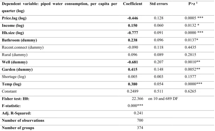
19 6.1. SONEDE-piped households

Table 3 shows results for SONEDE-piped households.

Dependent variable: piped water consumption, per capita per quarter (log) Coefficient Std errors P>z 1 Price.lag (log) -0.446 0.128 0.0005 *** Income (log) 0.150 0.060 0.0132 * Hh.size (log) -0.777 0.091 0.0000 *** Bathroom (dummy) 0.238 0.096 0.0137* Recent.connect (dummy) -0.090 0.118 0.4435 Rural (dummy) 0.096 0.089 0.2815 Well (dummy) -0.681 0.207 0.0010** Garden (dummy) 0.415 0.148 0.0052** Shortage (log) 0.005 0.003 0.1577 Temp (log) 0.380 0.054 0.0000*** Constant 0.2489 0.511 0.6265 Fisher test: H0: F-statistic: 22.366 0.000*** on 10 and 689 DF Adj. R-Squared: 0.241 Number of observations 700 Number of groups 374

Breush and Pagan Lagrangian multiplier test for random effects: H0: Var(u)=0, Chi2 358.39, Prob > chi2 : 0.000

1 _{Here ***, ** and * denote statistical significance at 0.1%, 1% and 5% respectively}

Table 3 Random effects water demand estimates for SONEDE-piped households

The demand function is significant at the 0.1% threshold, the coefficients of the variables retained are generally significant and all have the expected sign with regard to economic intuitions and the results of the literature relating to water demand. The null hypothesis in the Lagrange Multiplier Test - two-way effects (Breusch-Pagan) that the variance across individuals is zero was rejected. Coefficients have been corrected from heteroscedasticity. Significant differences across individuals confirm that there is a panel effect and that a component errors model is more appropriate than a simple OLS regression.

The simple significance tests demonstrate that households are price-sensitive: household price elasticity is estimated at -0.45 (significant at the 0.1% threshold), meaning that when the price increases by 10%, the quantity consumed falls by 4.5%. As expected, income elasticity is weakly positive at +0.15 (significant at the 5% threshold). The household size variable has a significantly negative impact on consumption, a fact that is in line with the literature: the larger the size of the family, the more the sharing between the members will reduce individual consumption. Temperature also positively impacts water consumption. The indicative variable indicating the

20

possibility of outdoor uses resulting from a vegetable garden is positive and significant. Similarly, owning a separate bathroom leads to increased consumption. The variables representing the age of the connection, the dummy for rural environment, the length of shortage and the possession of animals vary in the expected direction but are not significant.

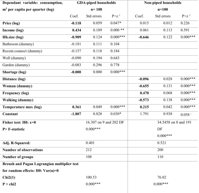
6.2. Non SONEDE-piped households

Table 4 describes the results of water demand function regressions for other households: GDA-piped and non-GDA-piped households.

Dependant variable: consumption, m3 _{per capita per quarter (log)}

GDA-piped households n= 108

Non-piped households n=100

Coef. Std errors P>z 1 _{Coef. Std errors P>z} 1

Price (log) -0.118 0.059 0.047* 0.015 0.012 0.226 Income (log) 0.434 0.109 0.000 ** 0.061 0.113 0.591 Hh.size (log) -0.909 0.124 0.000*** -0.646 0.122 0.000*** Bathroom (dummy) -0.181 0.111 0.104 Recent.connect (dummy) -0.157 0.118 0.184 Well (dummy) -0.090 0.194 0.643 Garden (dummy) -0.083 0.296 0.778 Shortage (log) -0.000 0.000 0.000*** Distance (log) -0.096 0.028 0.000*** Woman (dummy) -0.655 0.131 0.000*** Frequency (log) 0.470 0.068 0.000*** Walking (dummy) -0.573 0.138 0.000***

Temperature max (log) 0.361 0.049 0.000*** 0.215 0.042 0.000***

Constant -1.807 0.828 0.030* 1.791 0.938 _0.058 . Fisher test: H0: x=0 P> F-statistic 16.307 on 9 and 202 DF 0.000*** 34.5458 on 8 and 191 DF 0.000*** Adj. R-Squared: 0.401 0.521 Number of observations 212 200 Number of groups 108 110

Breush and Pagan Lagrangian multiplier test for random effects: H0: Var(u)=0

Chi2(1) P > chi2 100.53 0.000*** 76.02 0.000***

1 _{Here ***, **, *, and . denote statistical significance at 0.1%, 1%, 5% and 10%, respectively}

Table 4 Random Effects water demand estimates for GDA-piped and non-piped households Both of the demand functions are significant at the 0.1% threshold, the coefficients of the variables retained are generally significant and all have the expected sign with regard to economic intuitions

21

and the results of the literature relating to water demand. The null hypothesis in the Lagrange Multiplier Test - two-way effects (Breusch-Pagan) were rejected for both equations. Significant differences across individuals confirm that there is a panel effect and that a component errors model is more appropriate than a simple OLS regression. Coefficients have been corrected from heteroscedasticity.

The simple significance tests demonstrate that the GDA-piped households are significantly sensitive to prices, but only in a very weakly negative manner (-0.1 significant at the 1% threshold). Sensitivity to income is significantly positive (+0.3 significant at the 0.01% threshold). The shortage variable is significantly null, which is logical if we are aware of the practices of GDA-piped households: the taps are more often than not located at the edge of the plots and the households call on intermediate stocks when using the water (filling containers). During interruptions, the household consumes the intermediate stocks and the reserves from this source. The three last variables bathroom, recent.connect, well and garden are not significant.

With regard to non-piped households, price elasticity and income elasticities are not significant at the 5% threshold. It would seem that the pertinent variables are not price and income but variables relating to physical access to the resource. The accessibility of the source, using the proxy of frequency, is significant, as well as the variable indicating that a woman is responsible for collecting the water and the fact that water is transported on foot: the higher the frequency of water collection, i.e. the more it is accessible (to the person responsible for collection), the more consumption increases; when the woman is responsible for collecting the water, consumption falls and when animal-drawn or motorized transport solutions are not available, consumption decreases as well.

6.3. Discussion

We found that price and income elasticities change with the distribution system: price elasticity reach -0.45 for SONEDE piped-households and -0.12 for GDA-piped households and +0.15 and +0.43 respectively for income elasticity. In non-piped rural areas, water demand seems to be strongly driven by other variables characterizing the physical accessibility of water source: frequency of collection which indicates direct accessibility, distance to the source, people in charge of collecting water and mean of transport.

The findings of price elasticities for piped-households (SONEDE and GDA) can be compared to other studies conducted in developing countries, where values usually range from -0.3 to -0.6 for individual connections (Nauges & Whittington 2009). When looking more specifically at those conducted in the southern Mediterranean sub-region providing data from 1980 to 2008, we observe higher price elasticity values ranging from -0.2 to -0.8, with a number of outliers (Ben Zaied 2013, Sebri 2013, Binet & Ben Zaïd 2011, Ayadi et al. 2002, Zekri & Ariel Dinar 2003, Lahlou & Colyer

22

2000, Kertous 2012, GTZ customer survey, Makary Consulting, 2009, cited by USAID Egypt - Water Policy and Regulatory Reform 2012, Al–Najjar et al. 2011, Al-Karablieh et al. 2012, Salman et al. 2008).

Among them, only Zekri & Dinar (2003) investigates small systems; the authors present two extreme values calculated by a model based on aggregated data from 1983 to 1992 for rural Tunisia: -1.3 for households served by GDA (at this time access was only collective through water kiosks, there wasn’t any IC) against -0.2 for rural SONEDE-piped households. The authors explain this marked difference by the fact that GDA-households might be poorer than the others, and support their position with the water consumption level of each group: 63 m3 per year per household for GDA households and 137 m3 per year per household in SONEDE villages. In contrast, the four recent studies conducted at an aggregate level (the district level) in Tunisia exclusively in the SONEDE perimeter (Ben Zaied 2013; Sebri 2013; Binet & Ben Zaïd 2011; Ayadi et al. 2002) converge to show that small consumers are still less sensitive than larger ones and that it could be explained because they are mostly low-income households whose consumption is the minimum level necessary to meet basic needs. Some authors note also that it is possible that the highest price elasticity observed for bigger consumers can be explained by a higher average price charged: this can be a correct explanation, the study of Binet & Ben Zaïd (2011) shows that the average price paid by small consumers (less than 40 m³ per quarter between 1980 and 2008) is markedly lower than the tariff rate applied to larger consumer bills (US $ 0.2 / m³ against 0.5 US $ / m³).

Even if the present study is conducted at an individual scale (and not like the previous ones at the district level in the SONEDE perimeter), we can apply the same reasoning at our results. The much low price sensitivity for GDA-piped households, compared with SONEDE-piped households, and even null sensitivity for non-piped households, can be explained by their very low consumption levels which tend to incompressible water needs. Water consumption level for non-SONEDE households are much lesser, due to a poorer quality of drinking-water supply and a lower availability of water resource. The second argument is that SONEDE-piped households are charging a pricing structure with very high prices when water consumption rises which may make households more sensitive to price than a volumetric pricing structure with a constant proportional part. Lastly, payment frequency may also explain part of the difference in price sensitivity. SONEDE-piped households face a quarterly invoice, GDA-piped households a monthly or bi-monthly bill, while most of the non-connected households pay on a daily basis. The burden of the water bill may be more bearable when it is paid little by little, on a daily basis, rather than when it has to be paid once for a quarter consumption, amounting several tens of dinars.

23 7. Conclusion and Policy Implications

This studies sets in the general framework of southern Mediterranean countries facing, on the one hand, overexploitation and depletion of their water resources, and on the other hand, intensification of water demand due to population growth, mutations of water access modes and uses in rural areas. In the overall context of global warming, which may expand and lengthen droughts in the future, it is becoming crucial to improve the knowledge of water demand determinants, which may help in drawing and implementing the necessary regulatory tools including water pricing.

One key question in Tunisia is to anticipate SONEDE-piped households’ response to price change as water tariff will soon have to be increased. The current tariff does not cover current and future costs of water supply: SONEDE is already facing an unbalanced budget and this deficit will increase due to investing into new resources to be implemented (water transfer, desalination) to cope with increasing domestic water needs. Another important issue, which may also be answered by improved knowledge of water demand, concerns complementary tools to forecast water demand as well as wastewater volumes. In the Kairouan sub-region where groundwater is close to the surface, sanitation is also becoming a crucial issue for local authorities in rural areas: with a shift from collective access mode to private connection on the property, water consumption is constantly increasing and sustainable sanitation systems must be introduced to avoid polluting groundwater. This study endeavors precisely to improve the knowledge of water demand, both in urban and rural areas, by developing deep investigation to characterize water consumption level when there is no water meter. The results inform about differentiated price and income elasticities between areas and systems and other drivers in water demand. It is an important finding because it means that differentiated instruments could be more efficient, and also better target particular groups of consumers. Such a result could reopen the debate on the national pricing principle held since SONEDE creation and also the question about tariff equalization which had been questioned by Touzi et al. (2010) but could be subject of further analysis.

Thanks

This research work is carried out within two research projects financed by ANR programs: Arena (ANR-11-CEPL-0011) and Amethyst (ANR-12-TMED-0006-01). The authors are grateful to Bernard Barraqué (AgroParisTech – UMR CIRED) for his detailed comments and Stefano Farolfi (Cirad – UMR G-Eau) for his helpful advices.

References

Al-Karablieh, E. et al., 2012. The Residental Water Demand Function in Amman-Zarka Basin in Jordan. Wulfenia, 19(11), p.10.

24

in Greater Amman Area. Jordan Journal of Agricultural Sciences, 7(1), pp.93–103. Arbués, F., Garcia-Valinas, M.A. & Martinez-Espiñeira, R., 2003. Estimation of residential

water demand: a state-of-the-art review. Journal of Socio-Economics, 32(1), pp.81–102. Available at: D:\Biblio\Arbues&al_2003.pdf.

Ayadi, M., Krishnakumar, J. & Matoussi, M.S., 2002. A Panel Data Analysis of Residential Water Demand in Presence of Nonlinear Progressive Tariffs. Cahiers du département

d’économétrie, Faculté des sciences économiques et sociales, Université de Genève,

2002.06, p.32.

Baltagi, B., 2008. Econometric Analysis of Panel Data 4, illustr. John Wiley & Sons, ed., Basani, M., Isham, J. & Reilly, B., 2008. The Determinants of Water Connection and Water

Consumption: Empirical Evidence from a Cambodian Household Survey. World

Development, 36(5), pp.953–968. Available at:

http://www.sciencedirect.com/science/article/pii/S0305750X08000193.

Baumann, D., Boland, J. & Hanemann, M., 1998. Urban Water Demand Management and

Planning, USA: McGraw Hill.

Binet, M. & Ben Zaïd, Y., 2011. A seasonal integration and cointegration analysis of residential water demand in Tunisia. Working Paper, University of Rennes 1, CREM-CNRS, WP 2011-22(November), pp.1–19.

Dalhuisen, J.M. et al., 2003. Price and income elasticities of residential water demand: a meta-analysis. Land Economics, 79(2), pp.292–308.

Espey, M., Espey, J. & Shaw, W.D., 1997. Price elasticity of residential demand for water: a meta-analysis. Water Resources Research, 33(6), pp.1369–1374.

Espey, M., Espey, J. & Shaw, W.D., 1997. Price Elasticity of Residential Demand for Water: A Meta-Analysis. Water Resources Research, 33(6), pp.1369–1374. Available at: http://dx.doi.org/10.1029/97WR00571.

Gana, A., 2012. The Rural and Agricultural Roots of the Tunisian Revolution: When Food Security Matters. International Journal of Sociology of Agriculture and Food, 19(2), pp.201–213.

Hewitt, J.A. & Hanemann, W.M., 1995. A Discrete/Continuous Choice Approach to Residential Water Demand under Block Rate Pricing. Land Economics, 71(2), pp.173– 192. Available at: http://www.jstor.org/stable/3146499.

House-Peters, L.A. & Chang, H., 2011. Urban water demand modeling: Review of concepts, methods, and organizing principles. Water Resources Research, 47(5), p.W05401.

25

Kertous, M.. b, 2012. La demande en eau potable est-elle élastique au prix ? Le cas de la Wilaya de Bejaia. Revue d’Economie du Developpement, 26(1), pp.97–126. Available at:

http://www.scopus.com/inward/record.url?eid=2-s2.0-84862203135&partnerID=40&md5=58881b94360423ce9fd10566bbfac220.

Lahlou, M. & Colyer, D., 2000. Water conservation in Casablanca, Morocco. Journal of the

American Water Resources Association, 36(5), pp.1003–1012.

Ben Mansour, M., 2014. Personnal communication, Tunis.

Montginoul, M., Neverre, N. & Rinaudo, J.D., 2009. Simulating the impact of price level and structure on urban water demand - A Southern France case study. In Economics

instruments to support water policy in Europe. Paris, FRA, p. 19.

Nauges, C. & van den Berg, C., 2009. Demand for Piped and Non-piped Water Supply Services: Evidence from Southwest Sri Lanka. Environmental and Resource Economics, 42(4), pp.535–549. Available at: http://dx.doi.org/10.1007/s10640-008-9222-z.

Nauges, C. & Strand, J., 2007. Estimation of non-tap water demand in Central American cities.

Resource and Energy Economics, 29(3), pp.165–182. Available at:

http://linkinghub.elsevier.com/retrieve/pii/S0928765506000339.

Nauges, C. & Whittington, D., 2009. Estimation of Water Demand in Developing Countries: An Overview. The World Bank Research Observer, 25(2), pp.263–294.

Nordin, J.A., 1976. A Proposed Modification of Taylor’s Demand Analysis: Comment. The

Bell Journal of Economics, 7(2), pp.719–721.

OCDE, 2014. La gouvernance des services de l’eau en Tunisie : Surmonter les défis de la

participation du secteur privé. Études de l'OCDE sur l'eau Éditions O., Paris.

Salman, A., Al-Karablieh, E. & Haddadin, M., 2008. Limits of pricing policy in curtailing household water consumption under scarcity conditions. Water Policy, 10(3), pp.295–304. Sebri, M., 2014. A meta-analysis of residential water demand studies. Environment,

Development and Sustainability, 16(3), pp.499–520. Available at:

http://link.springer.com/10.1007/s10668-013-9490-9.

Sebri, M., 2013. Intergovernorate disparities in residential water demand in Tunisia: a discrete/continuous choice approach. Journal of Environmental Planning and

Management, 56(8), pp.1192–1211. Available at:

http://www.tandfonline.com/doi/abs/10.1080/09640568.2012.716366 [Accessed October 15, 2013].

26

de régulation tarifaire face aux défis futurs. Revue Tiers Monde, 203(juillet-septembre), pp.61–80.

USAID Egypt - Water Policy and Regulatory Reform, 2012. Cost Recovery and Pricing Models

- Policy Paper, Available at: http://wprregypt.com/Fetchpage.aspx?page=InternalDocs.

Worthington, A.C. & Hoffman, M., 2008. An Empirical Survey of Residential Water Demand Modelling. Journal of Economic Surveys, 22(5), pp.842–871.

Ben Zaied, Y., 2013. A long-run analysis of residential water consumption. Economics Bulletin,

33(1), pp.536–544. Available at:

http://medcontent.metapress.com/index/A65RM03P4874243N.pdf [Accessed October 16, 2013].

Zekri, S. & Dinar, A., 2003. Welfare consequences of water supply alternatives in rural Tunisia.

Agricultural Economics, 28(1), pp.1–12. Available at: