Product market regulation, innovation and productivity

(1)

HAL Id: halshs-00973947

https://halshs.archives-ouvertes.fr/halshs-00973947

Submitted on 4 Apr 2014

HAL is a multi-disciplinary open access archive for the deposit and dissemination of sci-entific research documents, whether they are pub-lished or not. The documents may come from teaching and research institutions in France or abroad, or from public or private research centers.

L’archive ouverte pluridisciplinaire HAL, est destinée au dépôt et à la diffusion de documents scientifiques de niveau recherche, publiés ou non, émanant des établissements d’enseignement et de recherche français ou étrangers, des laboratoires publics ou privés.

Product market regulation, innovation and productivity

Bruno Amable, Ivan Ledezma, Stéphane Robin

To cite this version:

Bruno Amable, Ivan Ledezma, Stéphane Robin. Product market regulation, innovation and produc-tivity. 2014. �halshs-00973947�

(2)

Documents de Travail du

Centre d’Economie de la Sorbonne

Product market regulation, innovation and productivity

Bruno AMABLE, Ivan LEDEZMA, Stéphane ROBIN

(3)

Product market regulation, innovation and

productivity.

Bruno Amable, Ivan Ledezma,

y

_{& Stéphane Robin}

z

March 2014

Abstract

Several recent policy and academic contributions consider that liberalising prod-uct markets would foster innovation and growth. This paper analyses the innovation-productivity relationship at the industry-level for a sample of OECD manufacturing industries. We pay particular attention to the vertically-induced in‡uence of prod-uct market regulation (PMR) of key input sectors of the economy on the innovative process of manufacturing and its consequences on productivity. We test for a di¤er-entiated e¤ect of this type of PMR depending on whether countries are technological leaders or laggards in a given industry and for a given time period. Contrary to the most widespread policy claims, the innovation-boosting e¤ects of liberalisation poli-cies at the leading edge are systematically not supported by the data. These …ndings question the relevance of a research and innovation policy based on liberalisation.

Keywords: product market regulation, innovation, productivity, growth Résumé: Plusieurs contributions récentes à la littérature académique et aux dé-bats de politique économique considèrent que la libéralisation des marchés de biens et services favoriserait la productivité et la croissance. Ce papier analyse la rela-tion entre innovarela-tion et productivité au niveau des branches pour un échantillon de pays de l’OCDE. Nous nous concentrons sur l’in‡uence verticale de la régle-mentation de marchés de biens et services dans certains secteurs d’inputs clés sur l’innovation et la productivité des secteurs manufacturiers. Nous testons un e¤et di¤érencié de la réglementation dans ces secteurs clés suivant que les pays sont des leaders ou des suiveurs technologiques dans un secteur donné pour une années don-née. Contrairement aux prescription de politique économique les plus répandues, les résultats empiriques ne valident en aucun cas l’existence d’e¤ets pro-innovation des politiques de libéralisation pour les leaders technologiques. Ces résultats remettent en question la pertinence d’une politque de recherche et d’innovation fondée sur la libéralisation.

Mots-clés: réglementation des marchés de biens et service, innovation, produc-tivité, croissance

JEL: D24, O43

University Paris I Panthéon - Sorbonne, CEPREMAP & IUF

y_{University of Paris-Dauphine, LEDa & IRD, UMR225-DIAL}

(4)

1 Introduction

The interest in policies aiming at fostering innovative activity through framework con-ditions has grown in Europe over the last decade, if only because restrictions on public spending have reduced the funding of more traditional research and innovation policies (Blind 2012). The regulatory framework has been at the centre of economic policy de-bates and the most accepted view in economic policy circles, particularly in Europe, is that a more intense competition should be promoted through the implementation of a

less stringent product market regulation (PMR).1 _{This view is not devoid of academic}

grounding. Following the emergence of the innovation-based endogenous growth theory (Aghion and Howitt, 1998), the importance of product market competition (PMC) as an engine of growth through its e¢ciency- and innovation-inducing e¤ects has been stressed in some theoretical and applied contributions (e.g. Aghion et al. 1997, 2005; Aghion and Gri¢th 2005; Aghion et al. 2014). This theme has been incorporated in the policy debates linking competition policy (or the extent of regulation in product markets) to competitiveness and growth. Indeed ’[t]he view that competition and entry should pro-mote e¢ciency and prosperity has now become a common wisdom worldwide’ (Aghion and Gri¢th, 2005, p.1). Moreover, the importance of competition as a driver of inno-vation and growth is expected to be greater for economies that compete at or near the leading edge of technology (Acemoglu et al. 2003, 2006; Vandenbusche et al., 2006). This literature has led European policy-makers to base their innovation-promoting e¤orts on the aforementioned less stringent PMR. This makes for a minimal technology and indus-trial policy, which merely consists in lifting regulations as much as possible to ensure a fair competition. However, putting too much emphasis on this "common wisdom" might in the end prove ine¢cient for innovation and growth, since it leaves little scope for a dedicated science and innovation policy (of the kind advocated by Dosi et al., 2006, for instance).

Meanwhile, the deregulation process is going on, more markedly in some industries than in others. In fact, since the 1980s (and mostly during the 1990s in Europe), net-work industries such as electricity, gas, rail, airlines, post and telecommunications have experienced an important process of market reform. The in‡uence of PMR in network industries is likely to impact the technological and competitive processes of the rest of the economy through vertical linkages, beyond what can be called the static aspects of com-petition such as prices, tax schedules or the scope of economies of scales (Armstrong and Sappington 2006, 2007). Thus, the transformation in the regulation of these industries has been seen as a wider liberalisation trend in developed economies. Some applied works (e.g. Bourlès et al., 2013) have concluded that this type of reforms has boosted produc-tivity growth. This link is widely perceived as robust and has recently been presented as evidence of the above-mentioned theoretical predictions. The underlying rationale is that the lack of dynamism in key input sectors of the economy becomes an impediment for …rms to implement their innovative strategies in their own markets, especially when they compete neck-and-neck with their rivals and seek to escape competition.

This paper critically examines the robustness of such claims, which have clear policy implications. Indeed, they are at the root of recommandations that advocate the liber-alisation of product markets as an innovation-boosting policy. The contribution of our

1_{For instance: the European Council recommendations in the context of Europe 2020 growth strategy}

(5)

critical examination is twofold. We …rst start by recalling the theoretical ambiguities of the relationship between competition and innovation. These go beyond the mechanisms isolated in models à la Aghion et al. (2005), such as the "escape competition" e¤ect. A review of the related empirical literature also reveals that results are fairly less clear-cut than what the "common wisdom" presumes. We then provide a systematic empirical assessment of the vertically-induced impact of non-manufacturing regulation (mainly in network sectors) on innovation and productivity in the manufacturing industries. Besides challenging the "common wisdom", this paper goes one step further in the empirical iden-ti…cation of the impact of regulatory reforms on technical progress. Most papers on this topic perform estimations based on reduced-form equations with productivity (or, less frequently, innovation) measures as the dependent variable. Here, we seek to add more structure to the econometric model by relating PMR to innovation, and the latter to productivity in an integrated framework.

We take inspiration from a large body of empirical work, starting from Griliches (1979, 1992, 1994, 2000) to recent studies derived from Crépon et al. (1998) who proposed a conceptual and analytical framework relating R&D, innovation and productivity at the …rm level. Di¤ering from this literature, our empirical application is performed at the industry level and focuses on the innovation-productivity nexus only. It relies on a sample of 13 manufacturing industries for 17 OECD countries during the 1977-2005 period, for which we have information on multifactor productivity, innovation, skill composition of labour and regulatory indicators. There are several reasons for performing our test at this level of aggregation.

First, the industry-level scope is more likely to capture information on equilibrium relationships. Thereby, this level of analysis is more relevant to measure the bottom-line aggregate impact on innovation and productivity of the (a priori) contradictory economic mechanisms induced by the competitive process. Second, it also facilitates the empirical implementation since at this level of analysis we do not face the selection issues that plague most …rm-level data on R&D. Moreover, industry-level data allows us to exploit the variability of di¤erent PMR regimes. This helps us reduce the risk of endogeneity as compared with observed measures of competition. Interpretations are more easily related to policy. We consider the same PMR indicators used in the related empirical literature. They are constructed by the OECD in order to capture the so-called "knock-on" e¤ects of non-manufacturing regulation on the rest of the economy. In the literature, these PMR indicators are used to measure the restrictiveness and low-competition environment supposedly induced by PMR.

Our measure of innovative performance is patenting intensity, which is a¤ected by PMR and in turn explains productivity. Using relative performances in total factor pro-ductivity, we also construct a measure of the closeness to the world technology frontier and split our sample into two unbalanced panels of national industries, depending on whether they perform near (leaders) or far from (followers) the leading edge. This allows us to test for a di¤erentiated impact of the regulatory environment on the technological change of each type of industry. In this new and extended approach, using recently issued data, results are consistent with previous …ndings contradicting the idea that technical progress at the leading edge should be grounded on liberalisation policies (e.g. Amable et al. 2010).

The paper is organised as follows. Section 2 summarises the current debate and …ndings on the relationship PMC, PMR, innovation and productivity growth. Section 3

(6)

presents the empirical strategy followed in the paper. Section 4 discusses the estimation results. A brief conclusion on policy implications is given in Section 5

2 PMC, PMR, innovation and productivity

Key EU policy initiatives, such as the Lisbon Agenda after 2005 or Europe 2020, rely on a couple of simple ideas. The …rst is that liberalisation would open markets to competition, allowing new entrants to bring new ideas and to challenge incumbents. The second is that this competitive pressure would stimulate innovation because companies facing com-petition would constantly need better products and services in order to maintain or gain market share (Ellersgaard Nielsen et al. 2013). Explaining the contribution of competi-tion policy to Europe 2020, Alexander Italianer, Director-General of the DG Competicompeti-tion declared in 2010 that competition was the key to ensure that the vision of growth and dynamism carried by Europe 2020 comes true: ’E¤ective competition pushes companies to innovate. They have to come up with new and better products to retain existing customers and gain new ones... Competition encourages companies to allocate their resources in the most e¢cient way, leading companies to o¤er more choice and better quality at lower

prices. As a result competition boosts productivity, growth and job creation.’ 2 In order

to better understand the policy debate on these issues, as well as our own critical con-tribution, it is worth making a selective synthesis of the main arguments analysing the link between market structure and technological performances. We begin by focusing the discussion on PMC as a theoretical concept and introduce PMR as the applied policy counterpart. It should be kept in mind, however, that the link between both remains far

from trivial.3

Although the contemporary "common wisdom" states that liberalising product mar-kets should foster innovation and productivity growth, theoretical contributions studying the way market structure shapes the incentives to innovate do not deliver an unambigu-ous positive relationship between PMC on the one hand and innovation or growth on the other. The "traditional" economic view is indeed one in which PMC has a negative impact on innovation as competition erodes innovation pro…ts (Schumpeter 1934, 1942). Such a negative link is featured in most endogenous growth models following the lines of Romer (1990), Segerstrom et al. (1990), Grossman and Helpman (1991) or Aghion and Howitt (1992).

By way of contrast, the managerial literature has provided arguments highlighting the role of competition as a slack-reducing device (Machlup, 1967; Porter 1990). When considering optimal (and not just satis…cing) behaviour, arguments mainly rely on the idea that PMC may reduce ine¢ciencies stemming from principal-agent governance-related problems. However, the resulting link between PMC and …rm e¢ciency is still usually ambiguous (Scharfstein; 1988; Hermalin, 1992; Schmidt, 1997; Raith, 2003).

When innovation occurs step-by-step, that is when laggards must catch-up with the technological leader before overtaking it, the above-mentioned Schumpeterian argument

2_{Competition Policy in support of the EU 2020 policy objectives. Speech at the Vienna Competition}

Conference 2010 ’Industry vs. Competition?’

3_{It is fair to say that the gap between de jure and de facto aspects of competition has been largely}

neglected in the applied macro-level policy oriented literature on PMR and growth. See for instance Armstrong and Sappington (2007) for a theoretical review on issues in the regulation of suppliers.

(7)

can be used to reverse the negative relationship between PMC and innovation in some industries. When laggards catch-up with the leader and both type of …rms compete in a neck-and-neck fashion, …rms will innovate in order to escape competition. However, at the same time, laggards’ innovation will be discouraged by competition as they anticipate lower post-innovation pro…ts. This is the underlying rationale of Aghion et al. (1997, 2005). Using this argument, the latter paper suggests that the relationship between PMC and innovation is hump-shaped and that the peak of this curve is ’larger and occurs at a higher degree of competition in more neck-and-neck industries’ (Aghion et al, 2005, Proposition 5), that is to say in industries where …rms compete at the same technological level. This has given rise to the idea that the bene…ts of increasing competition through lowering regulation should be higher near the world technological frontier, whereas they

could be nil or even negative far from that frontier.4

The nonlinearity of the relationship between competition and innovation is more gen-erally analysed by Boone (2001), who axiomatically de…nes the intensity of competition in order to encompass di¤erent standard parametrisations. Considering heterogenous com-petitors, Boone (2001) shows that the value of innovation changes with the identity of the innovator, which in turn depends on the level of competition itself. No general form of nonlinearity can be inferred without specifying the market structure in more details. Details therefore matter and it is not surprising to …nd contradicting claims when one goes further into the industrial organisation literature. For instance, within the context of Cournot competition with product di¤erentiation, Tishler and Milstein (2009) show that strategic behaviour in what they call R&D wars leads to a (non-inverted) U-shaped relationship.

As it is clear from Boone (2001), the possibility of innovation by technology leaders is key to understanding the e¤ect of PMC. Leaders may have some advantages that allow them to innovate despite the implied destruction of their own rents (the so-called ’Ar-row e¤ect’). One special form of leader’s advantage is that given by its position as an incumbent that moves …rst (Gilbert and Newberry, 1982). In that case, entry becomes endogenous and, contrary to traditional innovation-based growth models, leaders inno-vate and may remain in the market durably. Competition for the market can then be a substitute for competition in the market (Etro, 2007). The main idea here is that the presence of an active monopoly can actually hide an intense competition threat. Amable et al. (2010) show that even in a framework similar to Aghion et al. (2005), the possibility for the technological leader to innovate in order to make the follower’s innovation more di¢cult leads to a reversal of the relationship between competition and innovation in the so-called neck-and-neck industries: competition may become detrimental to innovation, even more so as one moves closer to the technological frontier. Moreover, the relationship between PMR and market structure itself is also a¤ected by these strategic interactions in a non-trivial way. Ledezma (2013) shows that, if the persistence of leadership relies on technological advantages strategically acquired by leaders in the process of innovation, PMR may in some cases reduce such advantages and induce …rm and innovation dynam-ics through Schumpeterian leapfrogging. PMR may in fact, purposedly or not, induce knowledge standardisation and this can be so even if PMR is theoretically allowed to increase the costs of innovation, as long as it forces leaders to stay, qualitatively, within

4_{Hölzl and Janger (2014) test the validity of the distance to the frontier argument for innovation in}

Europe and show that …rms close to the technological frontier increasingly rely on the creation of own knowledge for their innovation-based growth strategies.

(8)

the boundaries of the current good.

Implications of endogenous entry and strategic interactions render visible the weakness of outcome measures of competition or market concentration and explain the widespread use of regulatory indicators in the applied literature. Some contributions estimate the impact of PMR on innovation or productivity without taking into account the proximity to the technological frontier. Blind (2012) distinguishes several regulatory indicators derived from business opinion surveys and tests their impact on the patenting intensity at the macro-level for a panel of 21 countries between 1999 and 2004. His …ndings display a diversity of in‡uences according to the indicators. While restrictive price regulation has a negative impact on patenting, competition legislation has no impact, and product and service legislation, taken to deter business activity, actually has a positive in‡uence on a country’s innovative performance. Barbosa and Faria (2011) focus on 10 EU countries and 22 2-digit manufacturing industries. Their cross-section estimates for the period 2002-2004 show a weakly signi…cant negative e¤ect of regulation on the proportion of innovative …rms within an industry. However, they use a macroeconomic indicator of PMR, common to all industries of a given country. Empirical assessments at the industry-level using regulation policy measures are then useful to analyse the relevance of the received argument about the positive e¤ect of liberalisation on innovation and productivity growth.

A fairly large body of empirical literature follows this approach (see, e.g., Nicoletti and Scarpetta, 2003; Conway et al., 2006; Bourlès et al., 2013). It usually relies on time-varying industry-level data for developed countries. As in this paper, these works use PMR indicators constructed by the OECD, which tabulates detailed surveys on regulatory practices (see Section 3.1.2.). The scope of these practices is generally economy-wide or related to the experience of PMR in network services sectors. As a way to obtain more insights on the e¤ect of this latter type of reforms on the rest of the economy, the OECD constructs "regulatory impact" indicators that measure the so-called "knock-on" e¤ects of non-manufacturing regulation. This is done by connecting the regulatory practices in key non-manufacturing input sectors to the use of these sectors’ output in each industry of the economy. This is why regulatory impact indicators are usually presented as capturing the extent to which upstream regulation restrict activities in downstream industries. The resulting index of regulation is generally highly correlated with other aspects of PMR measured by economy-wide indicators (Amable et al. 2010) and at the same time allows for more time-variability across countries and industries: it is now possible to perform estimations on PMR data presenting a panel structure where individuals are country-industry couples (national industries), as it is the case with most of recently publicly available measures of technological performances.

In general, estimations seek to measure the impact of PMR on economic performance (captured by a measure of innovation or, more often, productivity) in a reduced-form econometric equation. The latter usually includes a measure of the gap vis-à-vis the technology frontier and a term interacting this technology gap with the PMR proxy. In many cases, the technology gap variable is in fact a measure of closeness to the technology frontier as the productivity of a country in a given industry and year is expressed relative to that of the best performing country (in the same industry and year). The interaction term indicates then how the marginal e¤ect of PMR (on economic performance) varies with the closeness to the technology frontier. This type of speci…cation is related to the

(9)

above-discussed conclusion of Aghion et al. (2005).5

Contradicting these …ndings, the results of Amable et al. (2010) show that the mar-ginal e¤ect of PMR on patenting intensity tends to be positively growing with the close-ness to the technological frontier. Furthermore, at the leading edge this marginal e¤ect is signi…cantly positive for several speci…cations. Although this result is not the rule in the related empirical literature it is by no means the exception. In practical terms, it comes from a positive estimated coe¢cient of the interaction term between PMR and the closeness to technology frontier. The same positive sign has also been found in Nico-letti and Scarpetta (2003) and Conway et al. (2006) with PMR indicators highlighting economy-wide aspects of PMR and productivity growth used as a proxy for technical progress/economic performance. Interpretations are however di¤erent: that positive sign in an error-correction model of multifactor productivity growth is seen as a slowing down e¤ect of PMR on the natural catching-up process of laggards. On the other hand, Bourlès et al. (2013) do report a negative e¤ect of PMR, which grows stronger the closer to the technology frontier. Their sample consider both manufacturing and service sectors. Nicoletti and Scarpetta (2003) and Inklaar et al. (2008) highlight the speci…cities of both type of sectors, something that could explain the di¤erences in estimates across studies. Arnold et al. (2008) merge industry-level regulation data with …rm-level information. They also seek to identify a di¤erentiated e¤ect of PMR on productivity, but this time de…ned on whether …rms are above the productivity median at the national level. The estimated coe¢cient of this di¤erently speci…ed interaction term is negative.

What emerges from this snapshot of the related literature is that the relationship between PMC, PMR, innovation and productivity growth can fairly be considered as an open question, at least to the point of tempering the optimism of mainstream policy recommendations. This mixture of results also appears in microeconomic country-speci…c studies on PMC and innovation (e.g. Cohen et al., 2010). Case study evidence from the electricity sector in the UK also adds to a less optimistic view as liberalisation there has been associated with a decline in R&D e¤orts (Jamasb and Pollitt, 2011). All this suggests that the heterogeneity of national industries matters. It is then important to provide further empirical scrutiny by fully exploiting the panel structure of the data. We show through reduced-form estimates that the …xed-e¤ect structure adopted in the econometric model is a key issue in the speci…cations to be estimated. Moreover, "sub-indicators" of the regulatory impact indicator allow us to isolate the scope of government participation in network industries, and therefore to analyse further a key element of network industries transformation. Full privatisation was not always the strategy adopted for unbundling and this may have had consequences for the rest of the economy. We consider then di¤erent indicators of regulatory impact, including, excluding or isolating the scope of government implication. Hence, relative to the existing empirical literature at the industry-level , the paper o¤ers a more careful account of panel unobserved heterogeneity within a system equation (the innovation-productivity nexus) in which causality is more rigorously tested and where more economic channels can be accounted for. The detail of this analysis is presented in what follows.

(10)

3 Methodology

3.1 The data

3.1.1 Sources

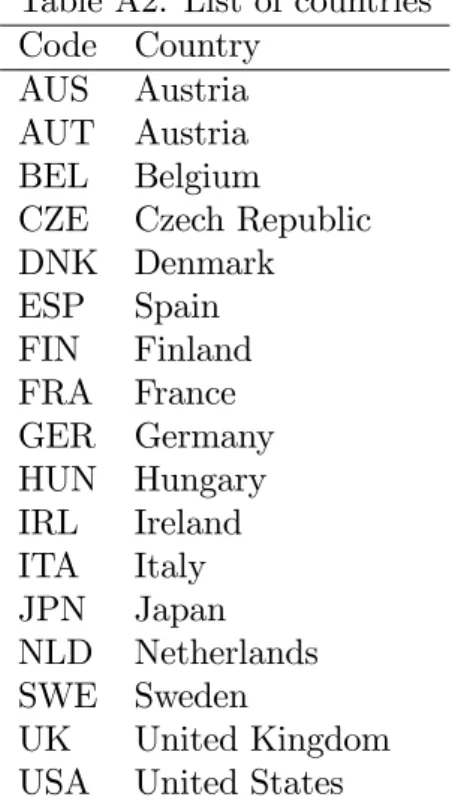
We use three main sources of industry-level time-series data. From the EU KLEMS database constructed by the Groningen Growth and Development Centre (GGDC), we draw information on labour inputs and multifactor productivity (MFP) measures. This information has been completed with data on patenting from EUROSTAT and with PMR indicators constructed by the OECD. We focus on manufacturing activities for which there exists available information on the main variables in our speci…cations. This leads to an unbalanced panel of 17 countries, 13 industries spanning from 1977-2005, which leads to more than …ve thousand potentially exploitable observations. Sample details are given in Appendix. Tables A1 and A2 present the lists of countries and industries. Aggregate descriptive statistics (mean, dispersion and number of non-missing observations) at the country level are reported in Table A3.

3.1.2 Main variables

MFP growth, MFP levels and closeness to the world technology frontier We

rely on measures of MFP growth relative to the base year 1995, available in the EU KLEMS database (March 2011 update of the November 2009 release). The use of EU KLEMS data on MFP growth is preferred to own custom calculations for several reasons. Methods and data are publicly available and continuously updated so that our analysis share a common accessible basis with other related studies. National Accounts are system-atically considered in EU KLEMS and completed with cross-checked micro level surveys, which increases information availability. At the same time the underlying methodology ensures conceptual consistency between variables and di¤erent scopes of aggregation. Im-proved availability is also gained in terms of detailed series on capital and labour inputs, which allows for a more precise growth accounting. Details on these and other features

of the EU KLEMS database can be found in O’Mahony and Timmer (2009).6

Our empirical strategy also requires MFP levels in order to construct an indicator of the closeness to the world technology frontier (WTF) which shall be used in our regres-sions to split the sample into "leader" and "follower" national industries. MFP levels were obtained combining (i) the MFP growth measures of EU KLEMS and (ii) the

Productiv-ity Levels (PL) database, also provided by the GGDC.7 _{The latter contains MFP indexes}

in levels relative to the United States only for the year 1997. This constraint is imposed by the need of o¤ering information comparable over time and across countries and in-dustries. To this aim, a speci…c de‡ation procedure is performed, which imposes heavy data requirements for constructing purchasing power parities (PPP) at the industry level. For this reason the PL database proposes measures in levels only for the benchmark year 1997, which is the best documented period for such a purpose. In addition, the resulting information on MFP levels also o¤ers a double de‡ation scheme for value added.

6_{For the data and further documentation see http://www.euklems.net/index.html and the numerous}

EU KLEMS publications dealing with particular applications as well methodological issues. O’Mahony and Timmer (2009) also present statistical comparisons with the OECD STAN database.

(11)

Using both the EUKLEMS and PL databases it is possible, however, to reproduce MFP series in levels for the full sample period. This amounts to apply the so called constant-PPP approach (see Inklaar and Timmer, 2008). More precisely, for a given

country c, industry i and time period t let MF P Gb

c;i;t be the MFP growth index relative

to the year base b; MF Pcit the MFP level index and MF PcitU S that relative to the United

States. In this notation, what the EU KLEMS and PL databases provide are, respectively

M F P G95 cit = M F Pcit M F Pci95 M F P_ci97U S = M F Pci97 M F PU Si97

MFP measures in levels for the full sample span are then obtained (after adjustment of the year base of the MFP growth index to 1997) as:

M F P_citU S = M F Pci97U S M F P G97 cit M F P G97 U Sit = M F Pcit M F PU Sit (1) With MFP levels at hand we de…ne our measure of closeness to the WTF as follows. For a given industry and time period we …rst identify the WTF as the highest MFP level observed in the sample, i.e. that of the leader country in the industry for the year of observation. Formally,

W T Fit = M F Pc itU S where c = arg max

c

M F P_citU S (2)

For each country c in a given industry i and time period t; the closeness to the WTF,

CLcit, is then de…ned as its MFP level relative to that of the WTF:

CLcit = M F PU S cit W T Fit = M F Pcit M F Pc it (3) As the last equality makes clear, the MFP level of the United States does not participate

in the de…nition of CLcit.

In our regressions, MF P G95

cit is used as the dependent variable and W T Fit belongs to

the set of explanatory variables. The constructed indicator of CLcit does not make part

of the set of covariates in the regressions. It is only used to identify subsamples of leaders and followers national industries.

Innovation Innovation is measured as patent intensity (PI), that is to say the

num-ber of patents divided by hours worked. Patent statistics relates to patent applications to the European Patent O¢ce (EPO) by sector of economic activity (EUROSTAT, Sci-ences & Technology database). Thanks to a concordance matrix between international patent classi…cation (IPC) and NACE classi…cation of economic activity (Rev 1.1), the statistics of patent applications can be distributed across industries for a given country (See Schmoch et al. 2003). Because of this distribution and the size-normalisation (with hours worked) we have a variable that is no longer an integer but a continuous aggregate indicator of innovation intensity.

Skill composition of labour Although the March 2011 update of the 2009 EU KLEMS

release provides information on labour inputs and labour compensation, the details on skill composition is only available in the previous release (2008). We extract from this latter

(12)

source the share of hours worked by high-skilled persons in order to include it in our regressions as a potential determinant of innovation. As a result, the main estimations do not consider the years 2006 and 2007 for which we have no information on skill com-position. On the other hand, reduced form estimates shown in the preliminary analysis performed in Section 3.1 do exploit the full length of the sample for the main variables and deliver consistent conclusions.

Product market regulation PMR is measured through the regulation impact

(hence-forth REGIMP) indicator constructed by the OECD. We use the 2008 updated release

(see Conway and Nicoletti (2006) for the methodology details).8 _{REGIMP measures the}

knock-on e¤ect of regulation in key non-manufacturing (NM) input sectors on the rest of the economy. These input sectors include: (i) network services such as energy (elec-tricity and gas), transport (air, rail and road transport) and communications (post and telecommunications) - the regulation of which is captured by the ETCR indicator; (ii) retail distribution and professional services - the regulation of which is captured by the RBSR regulation; and (iii) …nance. Regulation in each of these activities is measured as an average composite of scores constructed upon qualitative information about regu-latory practices in several important "reguregu-latory areas". For ETCR, these areas cover entry, public ownership, vertical integration, price controls and market structure. Infor-mation here is available for the 1975-2007 period. For RBSR regulation, areas consider more speci…c restrictions on entry and conduct, and the data contains information for 1998, 2003 and 2008. Information on the …nancial sector has the lowest coverage (only for 2003). Scores in all indicators of NM regulation are coded accordingly to an increasing schedule (from 0 to 6) re‡ecting the restrictiveness imposed by regulatory provisions.

REGIMP seeks to capture the impact of these NM regulatory provisions on all eco-nomic sectors. For each 2-digit ISIC industry, REGIMP is computed as a weighted sum of NM regulation indicators, where weights re‡ect the use of the respective NM sector

as input.9 _{The requirements of NM sectors in each industry are in turn obtained from}

harmonised input/output matrices. PMR in a NM sector will have a stronger impact on a speci…c industry if it is heavily used in production. Given this vertical linkage, REGIMP is usually interpreted as associating regulation in "upstream" industries with operation "downstream", although it should be kept in mind that not all manufacturing industries are …nal goods and that not all NM sector output is used in production activities. That said, an important share of NM sector output is used for production in other sectors. Conway and Nicoletti (2006), based on the input/output tables, report shares ranging from 50 to 80% so that REGIMP does give a measure about the degree of restrictiveness imposed to manufacturing activities due to PMR in key sectors of the economy.

As previously mentioned, a key advantage of REGIMP is its panel variability, which is compatible with our set of variables. At the same time, it remains strongly correlated with other measures capturing more directly regulatory practices, but that have the drawback of being economy-wide indicators with scarce variability in both time and cross-section dimensions (see for instance PMR indicators used in Nicoletti and Scarpetta, 2003). The latest release of REGIMP data also o¤ers series restricted to the regulatory area of

pub-8_{www.oecd.org/economy/pmr.}

9_{NM regulation indicators must be mapped to a 2-digit ISIC classi…cation which implies in some cases}

a simple average of sub-indicators of regulation (e.g. the average of regulation in Post and regulation in Telecomunication for the ISIC sector 64 Post and telecomunication).

(13)

lic ownership (henceforth the RPO indicator) as well as series excluding this dimension (henceforth RWPO). We use these additional series as alternative PMR indicators in our robustness checks.

3.2 Empirical Strategy

We estimate a two-equation model that allows us to identify (i) the determinants of innovation and (ii) those of MFP (which include innovation itself). Among these de-terminants, the vertically-induced e¤ects of non-manufacturing PMR (henceforth PMR for brevity) is expected to play a crucial role, which may depend on whether national industries compete far from or close to the WTF. In the …rst-stage equation, patent

in-tensity of country c; in industry i at time period t 1; ln P Icit 1; is explained by its

own autoregressive process, the level of PMR, ln P MRcit 1, the share of hours worked by

high-skilled workers, ln HScit 1; and the MFP level exhibited by the WTF, ln W T Fit 1.

In the second-stage equation, the dependent variable is the log-di¤erence of MFP relative

to the base year 1995, viz. ln MF P G95

cit = ln M F Pcit ln M F Pci95, which is explained by

PMR, patent intensity and the MFP level of the WTF. Neither the autoregressive process of innovation nor the share of high-skilled labour are assumed to directly in‡uence the log-di¤erence of MFP (recall that the productivity accounting allowing to compute MFP as a residual has already taken into account input factors). Formally,

ln M F P G95

cit = 0+ 1ln P M Rcit 1+ 2ln P Icit 1+ 3ln W T Fit 1+ ci+ t+ "cit (4)

ln P Icit 1 = 0+ 1ln P M R_{cit 1}+ 2ln W T F_{it 1}+ 3ln HS_{cit 1}+Pm₌_k ln P I_{cit 1}

+ ci+ t 1+ cit 1

where ci; ci are individual (country-industry) unobserved …xed e¤ects; tand tare time

speci…c unobserved …xed e¤ects; and …nally "cit and cit the idiosyncratic disturbances.

In our regressions we consider alternatively = 3; 4 and 5. We use an instrument

variable (IV) and GMM approaches to estimate (4). In both cases we take into account the unobserved individual time-invariant heterogeneity by exploiting within-group variance. This implies that the productivity equation will in fact be estimated in levels (i.e. the

term ln MF Pci95 ln M F P G

95

cit = ln

M F Pcit

M F Pci95 at the left-hand side will be eliminated by

the within-group transformation). In estimating (4) we also consider the possibility of arbitrary heteroskedasticity and autocorrelation.

In order to identify a di¤erentiated e¤ect of PMR accordingly to the "neck-and-neckness" of the technological competition, our estimations consider two kind of sub-samples: leaders and followers. Leaders are de…ned as those country-industry couples performing above a certain percentile of the sample distribution of the closeness to the

world technology frontier, CLcit, de…ned by eq. (3). We consider in our regressions the

50th, the 60th and the 75th percentiles of the CLcit as alternative cuto¤ levels for the

sample splitting. In each case, we allow our parameter estimates to di¤er in each

sub-sample. The MFP level featured at WTF, ln W T Fit 1; is introduced as an explanatory

variable in both equations in order to control for technological externatilities.

By letting PMR participate in both equations, we can identify how PMR a¤ects MFP through patented innovation as well as through other type of non-patented innovative activity. With the sample splitting we can test how its in‡uence may vary according to

(14)

the technology lead of a country in a given industry and time period. The most received argument discussed above suggests that one should expect in the …rst stage equation

1 <0 for leaders and 1 >0 for followers, provided that 2 >0:

4 Results

4.1 Preliminary analysis

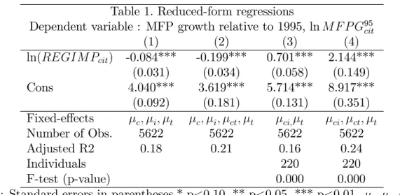
The three-dimensional structure of our data implies the presence of di¤erent sources of unobserved speci…cities explaining MFP di¤erences across national industries. We start therefore our analysis by estimating reduced-form regressions which seek to explain the log di¤erence of MFP by the log of our indicator of PMR (REGIMP) and a set of dummies controlling for time, country and industry …xed e¤ects, as well as their plausible interactions. Formally, we test:

ln M F P G95

cit = 0+ 1ln P M R_{cit 1}+ _cit (5)

where cit is composed of an intrinsical disturbance cit and several …xed e¤ects, the

speci…c form of which depends on the hypotheses regarding the underlying unobserved heterogeneity. Results are presented in Table 1. In column (1) the speci…cation considers

country, industry and time …xed e¤ects, i.e. cit = c + i + t + ict and yields a

signi…cantly negative elasticity of REGIMP. This result still holds and with increased magnitude (in absolute value) when the speci…cation includes country-speci…c time …xed

e¤ects, i.e. cit = c+ i+ t+ ct+ ict; which seeks to control for national-level shocks.

This type of dummy structure, controlling for national trends, is close to that assumed by Bourlès et al. (2013).

Column (3) and (4) report on speci…cations considering this time individual (country-speci…c industry) …xed-e¤ects. Regression in column (3) includes also time …xed e¤ects,

i.e. _cit = _ci+ _t+ ict , whereas country-speci…c time …xed e¤ects are added in the

re-gression reported in column (4), i.e. cit = ci+ ct+ t+ ict . Both of these speci…cations

are estimated using the within-group transformation. The Fisher test here indicates that we can reject at any conventional risk the null of no-joint e¤ect of individual (country-industry) intrinsic characteristics. In both of these regressions the elasticity of REGIMP is signi…cantly positive. This elasticity increases after the inclusion of country-time dum-mies, as in column (2). Hence, controlling for unobserved time-invariant individual het-erogeneity matters. Unobserved determinants of MFP tied to national industry-level speci…cities and correlated with our regulation proxy (e.g. institutions, initial conditions, technology-based R&D propensity, etc.) may lead to biased estimations if only indus-try characteristics common to all countries and/or counindus-try characteristics common to all industries are controlled for.

(15)

Table 1. Reduced-form regressions

Dependent variable : MFP growth relative to 1995, ln MF P G95

cit (1) (2) (3) (4) ln(REGIM Pcit) -0.084*** -0.199*** 0.701*** 2.144*** (0.031) (0.034) (0.058) (0.149) Cons 4.040*** 3.619*** 5.714*** 8.917*** (0.092) (0.181) (0.131) (0.351) Fixed-e¤ects c; i; t c; i; ct; t ci; t ci; ct; t Number of Obs. 5622 5622 5622 5622 Adjusted R2 0.18 0.21 0.16 0.24 Individuals 220 220 F-test (p-value) 0.000 0.000

Note: Standard errors in parentheses.* p<0.10, ** p<0.05, *** p<0.01. c; i; t; ci

and _ct stand for, resp., country, industry, time, country-speci…c industry and

country-speci…c time …xed e¤ects.

4.2 Two-step estimates

The results of the two-step analysis are presented in Tables 2 to 7. These tables report the estimation of eq. (4) for a subsample of leaders or followers national industries, de…ned di¤erently depending on whether they are respectively above or below the 50th, the 60th or the 75th percentile of our measure of closeness to the WTF (see section 2). All Tables show for a given type of individual (leader or follower) and regulation indicator (REGIMP, RWPO or RPO) the …rst-stage estimates (the patenting equation) in the upper panel and the second stage (the MFP equation) in the bottom panel. Columns (1) to (3) present estimations of the same model for a sample split at the 50th, 60th and 75th percentile respectively. Here, the lag of patenting intensity is instrumented by its own third lag. Columns (4) to (6) consider an additional scrutiny for the regressions of column (3), which is performed using the strictest de…nition of closennes to WTF. In this de…nition leaders are the national industries above the 75th percentile of WTF and followers those below, a sample split particularly interesting as it captures di¤erentiated e¤ects of PMR on what can be called the leading-edge of technology. These alternative regressions consider deeper autoregressive processes for patenting intensity. All models consider individual (i.e. country-industry) and time …xed e¤ects. In all regressions also, statistics are robust to arbitrary heteroskedasticity as well as to arbitrary autocorrelation through kernel-based estimations. Column (6) reports the results obtained from estimations implementing two-step e¢cient generalised method of moments (GMM).

The rows at the end of each table give a summary of tests on instruments as well as on identi…cation. These consist of (i) the Hansen test on the vailidity of overidentify-ing restrictions, (ii) a rank test for underidenti…cation based on a Lagrangean multiplier version of the Kleibergen and Paap (2006) rk statistic, which amounts to generalise the Anderson canonical correlation rank statistic to the non-i.i.d. case; (iii) a weak identi-…cation test which is a "robust" analog of the weak identiidenti-…cation IV test for the i.i.d. case (Stock and Yogo, 2005), based on the Kleibergen-paap rk statistics; and …nally (iv) a weak-identi…cation-robust inference test (i.e. a test on the structural signi…cance of the endogenous regressors) based on Anderson and Rubin (1949), here also considering

(16)

heteroskedasticity-robust statistics.10 _{Athough changing the regulation proxy or the}

sam-ple of national industries amounts to changing the scope of the regulatory provisions being considered and their expected impact on innovation and productivity, we keep the same speci…cation of instruments for the sake of comparison. The same structure of presentation is then kept in all tables.

The …rst estimations are made with the REGIMP indicator and the results are doc-umented in Table 2 for the leaders and Table 3 for the followers. The impact of PMR, measured by this proxy, is generally positive for leaders at both the innovation and the productivity stage. Interestingly, the point elasticity of PMR at the …rst stage (innova-tion) is positive but the parameter estimated is not signi…cantly di¤erent from zero at conventional levels in broad de…nitions of leader (i.e. national industries above the 50th and the 60th percentile of closeness to the WTF). However, this positive impact becomes signi…cant and signi…cantly higher when one narrows the de…nition of the leaders or, to put it di¤erently, when one goes nearer to the technology frontier: the elasticity jumps from 0.080 at the 50% split to 0.486 at the 75% level. Even in the fully instrumented model (columns (5) and (6)) the estimated elasticity is more than four times higher at the 75th percentile split. The instrumentation strategy is also validated for the 60% and the

75% threshold.11 _{Therefore, contrary to the common wisdom, these estimations show that}

PMR has a positive impact on innovation, which grows with the proximity to the WTF. As expected, skilled labour also favourably in‡uences innovation, which is also positively a¤ected by past innovation performance. On the other hand, spillovers stemming from the WTF appear to not signi…cantly a¤ect innovation for leader national industries. At the second stage (productivity), innovation is seen to positively in‡uence productivity in all regressions, with an elasticity that does not vary signi…cantly with the de…nition of the leader/follower split in the basic regressions. The positive impact of patents on productiv-ity should dispel any doubts one might have had about the relevance of that variable for representing signi…cant innovations. The introduction of the productivity externality term appear with a signi…cantly positive coe¢cient, but only at the vicinity of the WTF. For this subsample the value of the innovation elasticity is higher. The productivity equation also shows that PMR positively impacts productivity by other channels than innovative patented activity. Although in this stage the associated elasticity of PMR is signi…cantly positive and sizeable everywhere, it is also larger at the leading edge.

The results for the followers are documented in Table 3. The elasticity of PMR at the innovation stage is signi…cantly negative for every sample split, and less negative at the 75% cuto¤ level than at the 50% or the 60% cuto¤ levels. Combining this with the results obtained for the leaders, one obtains a signi…cantly negative in‡uence of PMR far from the technology frontier that gradually turns into a signi…cantly positive impact that grows when one gets near the technology frontier. This is exactly the opposite of the relationship postulated by the "common wisdom". Our results are nevertheless in accordance with those of Amable et al. (2010), Nicoletti and Scarpetta (2003) and

Con-10_{Whereas for the Hansen test we would like to fail to reject the null hypothesis that orthogonality}

conditions are valid, for the rest of tests the rejection of the respective null hypothesis is evidence of proper speci…cation.

11_{The higher p-values, yet still small, for the Anderson-Rubin tests are the consequence of the joint}

hypothesis tested: the coe¢cient of the endogenous regressor in the structural equation is equal to zero, and, in addition, the overidentifying restrictions are valid. As can be seen in Table 2, the coe¢cients of the lagged patenting intensity is itself signi…cant at least at the 10% level.

(17)

way et al. (2006).12 _{The fact that these results di¤er from what is generally seen as}

"common wisdom" illustrates how the relationship between PMR, innovation and growth is far from unambiguous. Depending on the proxies and econometric methodologies used, there is scope for some variety in the results. For instance, most empirical studies in the literature fail to develop suitable controls for unobserved individual heterogeneity, het-eroskedasticity and autocorrelation in the models from which they derive their results. In the present study, we not only use a carefully-constructed measure of MFP, we also im-plement an econometric methodology that controls for the above-mentioned biases (which may typically plague large panels in which the time dimension is long).

Going back to our other results, we …nd that the other elasticities in the innovation equation are in conformity with expectations: a signi…cantly positive in‡uence of skilled labour and past innovation. The world productivity frontier here again does not exert a signi…cant impact. At the second stage, as expected, the in‡uence of innovation on productivity is not as high as with industry leaders. The estimate of the elasticity of productivity with respect to innovation is only signi…cant at 10% for the 50% and 60% cuto¤ levels (columns (1) and (2)) and, when signi…cant, less than a half of the innovation elasticity for leaders in comparable models. Interestingly also, ccontrary to what happens in the innovation stage, in the productivity equation PMR has a signi…cantly positive impact on the productivity of followers, and the elasticity is generally higher than that estimated for leaders. This suggests the presence of important non-patented innovative activity in this sub-sample.

(18)

Table 2.

Leaders - Innovation equation (…rst-stage estimates)- REGIMP indicator

Dependent variable: patenting intensity, ln(P Icit 1)

WTF split Q50 Q60 Q75 Q75 Q75 Q75 (1) (2) (3) (4) (5) (6) ln(REGIM Pcit 1) 0.080 0.100 0.486*** 0.406*** 0.331** 0.331** (0.101) (0.127) (0.152) (0.145) (0.143) (0.143) ln(W T Fcit 1) -0.030 -0.015 -0.022 -0.039 -0.033 -0.033 (0.030) (0.039) (0.053) (0.048) (0.045) (0.045) ln(P Icit 4) 0.491*** 0.459*** 0.393*** 0.339*** 0.299*** 0.299*** (0.023) (0.028) (0.034) (0.050) (0.057) (0.057) ln(P Icit 5) 0.135*** 0.186*** 0.186*** (0.047) (0.063) (0.063) ln(P Icit 6) 0.064 0.064 (0.040) (0.040) ln(HScit 1) 0.126*** 0.124*** 0.108** 0.135*** 0.147*** 0.147*** (0.039) (0.043) (0.048) (0.045) (0.043) (0.043) Adjusted R2 0.86 0.86 0.84 0.84 0.84 0.84

Leaders - Productivity equation (second-stage estimates)- REGIMP indicator

Dependent variable: MFP growth relative to 1995, ln MF P G95

cit (1) (2) (3) (4) (5) (6) ln(P Icit 1) 0.120*** 0.109** 0.135* 0.199** 0.221*** 0.171** (0.040) (0.045) (0.071) (0.078) (0.081) (0.075) ln(REGIM Pcit 1) 0.341*** 0.546*** 0.453*** 0.436*** 0.441*** 0.480*** (0.108) (0.126) (0.156) (0.157) (0.159) (0.157) ln(W T Fcit 1) -0.062 0.008 0.117** 0.113** 0.105* 0.117** (0.041) (0.043) (0.054) (0.054) (0.055) (0.054) Number of obs. 2528 2018 1262 1216 1169 1169 Individuals 150 130 87 85 84 84

Tests of instruments and identi…cation Overidentifying restrictions (Hansen test)

p-value (J statistic) 0.004 0.108 0.484 0.595 0.211 0.211

Under identi…cation (Kleibergen-Paap rank test )

p-value (LM statistic) 0.000 0.000 0.000 0.000 0.000 0.000

Weak identi…cation (Kleibergen-Paap based, for non-i.i.d errors)

Wald F statistic 233.18 140.327 71.818 62.053 54.231 54.231

Endogenous regressors (Anderson-Rubin test)

p-value (chi-2 test) 0.001 0.034 0.173 0.086 0.028 0.028

Note: Standard errors in parentheses.* p<0.10, ** p<0.05, *** p<0.01. See eq. (4) for details on the IV speci…cation. All estimations consider a constant term, individual (country-industry) …xed e¤ects and year dummies. Statistics are robust to arbitrary heteroskedasticity and also to arbitrary autocorrelation through kernel-based estimations. Column (6) reports two-step e¢cient generalised method of moments (GMM) estimations.

(19)

Table 3.

Followers - Innovation equation (…rst-stage estimates)- REGIMP indicator

WTF split Q50 Q60 Q75 Q75 Q75 Q75 (1) (2) (3) (4) (5) (6) ln(REGIM Pcit 1) -0.353*** -0.368*** -0.254*** -0.240*** -0.250*** -0.250*** (0.096) (0.087) (0.076) (0.072) (0.072) (0.072) ln(W T Fcit 1) -0.021 -0.020 0.001 -0.007 -0.020 -0.020 (0.020) (0.018) (0.017) (0.016) (0.015) (0.015) ln(P Icit 4) 0.436*** 0.449*** 0.481*** 0.423*** 0.370*** 0.370*** (0.029) (0.025) (0.021) (0.031) (0.034) (0.034) ln(P Icit 5) 0.150*** 0.130*** 0.130*** (0.027) (0.034) (0.034) ln(P Icit 6) 0.097*** 0.097*** (0.026) (0.026) ln(HScit 1) 0.030 0.038 0.089** 0.096*** 0.079** 0.079** (0.048) (0.039) (0.036) (0.034) (0.034) (0.034) Adjusted R2 0.82 0.83 0.85 0.85 0.84 0.84

Followers - Productivity equation (second-stage estimates) - REGIMP indicator

cit (1) (2) (3) (4) (5) (6) ln(P Icit 1) 0.058 0.054 0.069** 0.083** 0.093** 0.093*** (0.050) (0.043) (0.034) (0.036) (0.037) (0.034) ln(REGIM Pcit 1) 0.676*** 0.673*** 0.577*** 0.591*** 0.604*** 0.508*** (0.223) (0.185) (0.148) (0.150) (0.152) (0.130) ln(W T Fcit 1) 0.107*** 0.071** 0.025 0.013 0.010 -0.003 (0.038) (0.032) (0.027) (0.026) (0.027) (0.025) Number of obs. 2328 2843 3603 3478 3356 3356 Individuals 162 182 197 197 196 196

Wald F statistic 117.62 157.084 252.284 249.726 190.421 190.421

p-value (chi-2 test) 0.026 0.077 0.044 0.012 0.010 0.010

Note: Standard errors in parentheses.* p<0.10, ** p<0.05, *** p<0.01. See eq. (4) for details on the IV speci…cation. All estimations consider a constant term, individual (country-industry) …xed e¤ects and year dummies. Statistics are robust to arbitrary heteroskedasticity and also to arbitrary autocorrelation through kernel-based estimations. Column (6) reports two-step e¢cient generalised method of moments (GMM) estimations. To sum up, with the widely-used REGIMP indicator, PMR has been found to be a positive in‡uence on leaders’ innovation and a negative one on followers’. This is the opposite of the received view about the merits of deregulation policy for innovation

(20)

performance at the leading edge, but this is in accord with previous results discussed above (specially those by Amable et al. (2010)) and also with standard Schumpeterian mechanisms. Moreover, PMR has also a positive in‡uence on productivity and this time for both leaders and followers, which again contradicts the "common wisdom".

As explained in Section 2, the regulation proxy REGIMP is an aggregate index that summarises all areas of regulation covered in each sub-index of regulatory practices in network services, retail and …nance. In order to disentangle di¤erent channels by which product market provisions in these sectors a¤ect the rest of the economy, the OECD provides alternative indicators that either exclude the public ownership dimension (the aforementioned RWPO indicator), or isolate it (the aforementioned RPO indicator). We use these as alternative measures of regulatory pressures shaping the innovative activity of national industries.

Tables 4 and 5 present estimations performed with the RWPO indicator of regulation, respectively for leaders and followers. Regressions using this alternative indicator are interesting in that they help to identify whether the positive impact of PMR on innova-tion and productivity presented above relates to provisions shaping market structure (and thus the incentives to engage in innovative activities), or conversely to the presence of the State, which may have a particularly higher propention to engage in R&D investments (motivated for instance by wider public policies integrating the positive externalities of the innovation process). Measured by this indicator, PMR appears to impact innova-tion in a broadly similar fashion to that observed above using the REGIMP indicator. The signi…cantly positive in‡uence of RWPO on leaders’ innovation also appears in the vicinity of the WTF. The impact of RWPO on followers is mainly negative but less so as one moves closer to the leading edge. Therefore, the slope of the curve linking the PMR-elasticity of innovation to the proximity to the technological frontier is here again positive, and not negative as the common wisdom would have it. Regarding the other regressors of the …rst stage, we observe that the impact of the share of skilled labour is also similar to those obtained previously: positive for leaders’ innovation and lower and less signi…cant for followers’ innovation. Likewise, in this stage, spillovers stemming from the world technology leader are not signi…cantly di¤erent from zero. As for the productivity equation, innovation has a signi…cantly positive in‡uence on leaders’ productivity, and this time a non-signi…cant one for followers, which is consistent with the large p-values in the corresponding Anderson-Rubin tests. Using the RWPO indicator, PMR has almost no direct impact on followers’ or on leaders’ productivity. The world technological frontier externality has a positive impact on leaders especially when the closeness to the WTF is restricted to the 75%. Estimations using the RWPO indicator yield then a similar pattern regarding the innovation stage but a fairly weaker one regarding the productivity stage. Instrumentation is validated in terms of orthogonality and identi…cation for leading edge estimates.

Estimations are then performed with RPO which considers only the public ownership dimension. The results are featured in Tables 6 and 7 for leaders and followers respectively. As it was the case with the other PMR indicators, the impact of RPO on innovation is signi…cantly positive and increases with the proximity to the technological frontier. PMR presents here also a signi…cantly negative in‡uence on innovation with followers. Innovation for leaders also presents a sizeable positive and signi…cant impact, although it should be kept in mind that the same instrumenting strategy used in the previous tests in the productivity equation of leaders is not validated here by the test of exogeneity of

(21)

the instruments. The results of the innovation equation as a single equation, and namely the sign of the elasticities of the PMR indicator, of course are not concerned by this. For the productivity equation of followers when the sample is split at the 75th percentile, the exogeneity of instruments is broadly validated, especially in the full speci…cation. Here again, as in the case of REGIMP, PMR appears to positively in‡uence productivity for followers, even though is negatively associated with their patenting intensity. Overal, even if weaker in light of orthogonality conditions in the two-equation model for leaders, the evidence suggested by the RPO indicator by no means gives support to the postulate of a negative in‡uence of larger upstream public ownership on leading-edge technical progress. Indeed, the opposite can be concluded from the single innovation equation.

Therefore, the estimations made with the other indicators of vertically-induced PMR broadly con…rm the results obtained with REGIMP. Regulation has a positive in‡uence on innovation at the leading edge and, in several cases, directly on productivity as well. Besides, the relationship between the impact of PMR and the distance to the technological frontier that one can draw from the previous results contradicts the received view: PMR’s bene…cial e¤ects are stronger for industries that are closer to the frontier.

(22)

Table 4.

Leaders - Innovation equation (…rst-stage estimates)- RWPO indicator

WTF split Q50 Q60 Q75 Q75 Q75 Q75 (1) (2) (3) (4) (5) (6) ln(RW P Ocit 1) 0.076 0.074 0.329*** 0.342*** 0.368*** 0.368*** (0.081) (0.100) (0.121) (0.115) (0.113) (0.113) ln(W T Fcit 1) -0.039 -0.032 -0.032 -0.049 -0.045 -0.045 (0.030) (0.039) (0.055) (0.049) (0.046) (0.046) ln(P Icit 4) 0.493*** 0.463*** 0.409*** 0.354*** 0.308*** 0.308*** (0.024) (0.029) (0.036) (0.055) (0.064) (0.064) ln(P Icit 5) 0.136*** 0.189*** 0.189*** (0.050) (0.067) (0.067) ln(P Icit 6) 0.073* 0.073* (0.042) (0.042) ln(HScit 1) 0.076** 0.087** 0.085* 0.116*** 0.139*** 0.139*** (0.037) (0.043) (0.049) (0.045) (0.043) (0.043) Adjusted R2 0.87 0.86 0.85 0.84 0.84 0.84

Leaders - Productivity equation (second-stage estimates)- RWPO indicator

cit (1) (2) (3) (4) (5) (6) ln(P Icit 1) 0.121*** 0.124** 0.182** 0.254*** 0.273*** 0.238*** (0.042) (0.048) (0.073) (0.079) (0.083) (0.079) ln(RW P Ocit 1) 0.022 0.187* 0.158 0.145 0.144 0.151 (0.092) (0.110) (0.135) (0.134) (0.135) (0.132) ln(W T Fcit 1) -0.069* -0.004 0.109** 0.106** 0.098* 0.109** (0.042) (0.044) (0.054) (0.054) (0.055) (0.053) Number of obs. 2398 1917 1196 1154 1112 1112 Individuals 146 126 82 80 79 79

Wald F statistic 204.263 124.064 68.257 57.501 52.506 52.506

p-value (chi-2 test) 0.002 0.023 0.042 0.013 0.003 0.003

Note: Standard errors in parentheses.* p<0.10, ** p<0.05, *** p<0.01. See eq. (4) for details on the IV speci…cation. All estimations consider individual (country-industry) …xed e¤ects and year dummies. Statistics are robust to arbitrary heteroskedasticity and also to arbitrary autocorrelation through kernel-based estimations. Column (6) reports two-step e¢cient generalised method of moments (GMM) estimations.

(23)

Table 5.

Followers - Innovation equation (…rst-stage estimates)- RWPO indicator

WTF split Q50 Q60 Q75 Q75 Q75 Q75 (1) (2) (3) (4) (5) (6) ln(RW P Ocit 1) -0.222** -0.236*** -0.167** -0.111* -0.093 -0.093 (0.088) (0.080) (0.069) (0.067) (0.067) (0.067) ln(W T Fcit 1) -0.010 -0.016 0.001 -0.005 -0.016 -0.016 (0.021) (0.019) (0.018) (0.016) (0.015) (0.015) ln(P Icit 4) 0.432*** 0.446*** 0.473*** 0.416*** 0.358*** 0.358*** (0.030) (0.026) (0.022) (0.032) (0.035) (0.035) ln(P Icit 5) 0.155*** 0.126*** 0.126*** (0.028) (0.035) (0.035) ln(P Icit 6) 0.113*** 0.113*** (0.026) (0.026) ln(HScit 1) 0.037 0.039 0.069* 0.080** 0.058* 0.058* (0.050) (0.043) (0.037) (0.034) (0.032) (0.032) Adjusted R2 0.82 0.82 0.85 0.84 0.83 0.83

Followers - Productivity equation (second-stage estimates)- RWPO indicator

cit (1) (2) (3) (4) (5) (6) ln(P Icit 1) -0.008 -0.012 0.008 0.021 0.035 0.050 (0.048) (0.041) (0.034) (0.035) (0.036) (0.034) ln(RW P Ocit 1) 0.030 0.060 0.038 0.053 0.070 0.090 (0.100) (0.085) (0.071) (0.070) (0.070) (0.069) ln(W T Fcit 1) 0.090** 0.059* 0.016 0.005 0.000 -0.006 (0.037) (0.031) (0.027) (0.027) (0.027) (0.026) Number of obs. 2263 2749 3474 3358 3244 3244 Individuals 162 181 197 197 196 196

Wald F statistic 108.934 143.801 223.719 219.13 172.072 172.072

p-value (chi-2 test) 0.571 0.595 0.744 0.103 0.067 0.067

(24)

Table 6.

Leaders - Innovation equation (…rst-stage estimates)- RPO indicator

WTF split Q50 Q60 Q75 Q75 Q75 Q75 (1) (2) (3) (4) (5) (6) ln(RP Ocit 1) 0.153* 0.176* 0.489*** 0.342*** 0.212** 0.212** (0.080) (0.104) (0.106) (0.103) (0.107) (0.107) ln(W T Fcit 1) -0.022 0.001 -0.028 -0.037 -0.028 -0.028 (0.030) (0.039) (0.054) (0.049) (0.048) (0.048) ln(P Icit 4) 0.512*** 0.478*** 0.412*** 0.311*** 0.273*** 0.273*** (0.024) (0.030) (0.036) (0.055) (0.063) (0.063) ln(P Icit 5) 0.178*** 0.189** 0.189** (0.050) (0.075) (0.075) ln(P Icit 6) 0.087** 0.087** (0.044) (0.044) ln(HScit 1) 0.130*** 0.123*** 0.102** 0.112** 0.104** 0.104** (0.040) (0.044) (0.049) (0.047) (0.047) (0.047) Adjusted R2 0.86 0.86 0.83 0.82 0.81 0.81

Leaders - Productivity equation (second-stage estimates)- RPO indicator

cit (1) (2) (3) (4) (5) (6) ln(P Icit 1) 0.115*** 0.100** 0.172** 0.230** 0.259** 0.183* (0.043) (0.049) (0.082) (0.094) (0.103) (0.101) ln(RP Ocit 1) 0.243*** 0.356*** 0.162 0.144 0.145 0.177 (0.075) (0.085) (0.115) (0.121) (0.125) (0.120) ln(W T Fcit 1) -0.073 0.001 0.118* 0.115* 0.110* 0.114* (0.046) (0.049) (0.062) (0.062) (0.062) (0.062) Number of obs. 2277 1795 1075 1037 999 999 Individuals 145 124 83 81 80 80

Wald F statistic 237.382 134.879 67.345 50.004 36.444 36.444

p-value (chi-2 test) 0.000 0.004 0.008 0.008 0.003 0.003

(25)

Table 7.

Followers - Innovation equation (…rst-stage estimates)- RPO indicator

WTF split Q50 Q60 Q75 Q75 Q75 Q75 (1) (2) (3) (4) (5) (6) ln(RP Ocit 1) -0.192** -0.169** -0.072 -0.100 -0.131** -0.131** (0.095) (0.083) (0.069) (0.064) (0.062) (0.062) ln(W T Fcit 1) -0.028 -0.024 -0.002 -0.011 -0.025 -0.025 (0.020) (0.019) (0.018) (0.016) (0.016) (0.016) ln(P Icit 4) 0.454*** 0.468*** 0.494*** 0.426*** 0.376*** 0.376*** (0.030) (0.026) (0.022) (0.034) (0.036) (0.036) ln(P Icit 5) 0.160*** 0.157*** 0.157*** (0.030) (0.037) (0.037) ln(P Icit 6) 0.078*** 0.078*** (0.025) (0.025) ln(HScit 1) 0.044 0.051 0.096** 0.098*** 0.071** 0.071** (0.050) (0.041) (0.038) (0.035) (0.035) (0.035) Adjusted R2 0.83 0.83 0.85 0.85 0.85 0.85

Followers - Productivity equation (second-stage estimates)- RPO indicator

cit (1) (2) (3) (4) (5) (6) ln(P Icit 1) 0.023 0.016 0.042 0.056 0.067* 0.074** (0.049) (0.042) (0.034) (0.036) (0.036) (0.035) ln(RP Ocit 1) 0.605*** 0.558*** 0.458*** 0.490*** 0.521*** 0.445*** (0.177) (0.145) (0.113) (0.116) (0.120) (0.106) ln(W T Fcit 1) 0.105*** 0.069** 0.019 0.008 0.003 -0.012 (0.040) (0.034) (0.028) (0.028) (0.028) (0.027) Individuals 160 180 196 196 195 195

Wald F statistic 116.259 156.729 251.93 262.204 193.284 193.284

p-value (chi-2 test) 0.038 0.150 0.129 0.037 0.032 0.032