HAL Id: hal-01736454
https://hal.inria.fr/hal-01736454
Submitted on 28 May 2018
HAL is a multi-disciplinary open access
archive for the deposit and dissemination of
sci-entific research documents, whether they are
pub-lished or not. The documents may come from
teaching and research institutions in France or
abroad, or from public or private research centers.
L’archive ouverte pluridisciplinaire HAL, est
destinée au dépôt et à la diffusion de documents
scientifiques de niveau recherche, publiés ou non,
émanant des établissements d’enseignement et de
recherche français ou étrangers, des laboratoires
publics ou privés.
Cross-Sectional Data
Kristin Mcleod, Kristin Tøndel, Lilian Calvet, M Sermesant, Xavier Pennec
To cite this version:
Kristin Mcleod, Kristin Tøndel, Lilian Calvet, M Sermesant, Xavier Pennec. Cardiac Motion Evolution
Model for Analysis of Functional Changes Using Tensor Decomposition and Cross-Sectional Data.
IEEE Transactions on Biomedical Engineering, Institute of Electrical and Electronics Engineers, In
press, 65 (12), pp.2769 - 2780. �10.1109/TBME.2018.2816519�. �hal-01736454�
Cardiac Motion Evolution Model for Analysis of
Functional Changes Using Tensor Decomposition
and Cross-Sectional Data
K. McLeod, K. Tøndel, L. Calvet, M. Sermesant, X. Pennec
Abstract—Cardiac disease can reduce the ability of the ven-tricles to function well enough to sustain long-term pumping efficiency. Recent advances in cardiac motion tracking have led to improvements in the analysis of cardiac function. We propose a method to study cohort effects related to age with respect to cardiac function. The proposed approach makes use of a recent method for describing cardiac motion of a given subject using a Polyaffine model, which gives a compact parameterisation that reliably and accurately describes the cardiac motion across pop-ulations. Using this method, a data tensor of motion parameters is extracted for a given population. The partial least squares method for higher-order arrays is used to build a model to describe the motion parameters with respect to age, from which a model of motion given age is derived. Based on cross-sectional statistical analysis with the data tensor of each subject treated as an observation along time, the left ventricular motion over time of Tetralogy of Fallot patients is analysed to understand the temporal evolution of functional abnormalities in this population compared to healthy motion dynamics.
Index Terms—cardiac motion tracking, evolution modelling, tensor decomposition, N-way PLS, population statistics, atlas, non-rigid image registration, spatio-temporal alignment, Tetral-ogy of Fallot.
I. INTRODUCTION
Cardiovascular disease (CVD) is an ongoing problem glob-ally and research into the mechanisms behind CVD is evolving continuously. This has led to novel therapies being developed regularly in response to this growing knowledge. Despite this, for certain diseases relatively little is known about the progres-sion of the disease. Knowing how a patient will respond to a given treatment (or in absence of any treatment) is an impor-tant factor in clinical decision-making in order to optimise pa-tient care. However, understanding complex dynamics such as those observed in the heart (hemodynamics, electrophysiology, structure, and mechanics for instance), remains a challenging
Copyright c 2018 IEEE. Personal use of this material is permitted. How-ever, permission to use this material for any other purposes must be obtained from the IEEE by sending a request to [email protected].
K. McLeod was with the Computational Cardiac Modelling Group, Simula Research Laboratory, Oslo 1364, Norway and is now with the Cardiovascular Ultrasound division of GE Healthcare, Horten 3183, Norway (correspondence email: [email protected])
K. Tøndel was with the Computational Cardiac Modelling Group, Simula Research Laboratory, Oslo 1364, Norway and is now with the Faculty of Science and Technology, Norwegian University of Life Sciences, ˚As 1432, Norway.
L. Calvet was with the Media Programming Group, Simula Research Laboratory, Oslo 1364, Norway and is now with the EnCoV/IP group, CHU Clermont Ferrand, Clermond Ferrand 63000, France
M. Sermesant and X. Pennec are with the Asclepios Research Group, Inria, Sophia Antipolis 06902, France
task. Determining how these complex dynamics will evolve over time is even more difficult, and yet knowing how the heart re-models under different circumstances is crucial to optimise the timing of interventions and for determining which therapy is optimal (in terms of long-term outcome) for the patient. In this paper we propose a method to statistically model cohort effects related to age on cardiac motion dynamics. Further, assuming that cohort effects can reflect longitudinal effects, a model of cardiac function at different ages is used as a first attempt to analyse the evolution of the heart over time.
A. Related Work
Cardiac function (in terms of mechanical pumping effi-ciency) is affected by a number of cardiac diseases, and for this reason it has been studied in recent years both from clinical and computational points of view by using signals and images to determine quantitative measures of function. For example, electrocardiogram (ECG) can be used to examine the electrical activity of the heart and to assess heart rhythm. Imag-ing (cardiovascular magnetic resonance (CMR), computed tomography (CT), echocardiography (ECHO)) can be used to assess morphology, mechanical function, hemodynamics, and for tissue characterisation. Clinical measures of mechanical function are predominantly based on quantifying global prop-erties such as volumes, diameters, ejection fraction, or regional measures such as stress/strain. Computational methods have been developed in recent years to go beyond these global or regional measures in order to provide more comprehensive evaluations of cardiac function by studying the full motion dynamics as the heart beats.
1) Computational Cardiac Function Analysis: Several
computational methods for quantifying cardiac function using non-rigid image registration techniques have been developed in recent years (see [1], [2] for a review of some earlier methods). More recent techniques include statistical shape modelling [3] and [4], and atlas-based regional wall motion analysis [5]. A common constraint used in state-of-the-art methods to retain physiological motion dynamics is to enforce the deformations (which describe the motion from one image to another) to be diffeomorphic (smooth transformations that preserve the structure of the material to prevent non-physiological trans-formations such as folding). Many methods also constrain the deformations to be incompressible or near-incompressible to account for the fact that cardiac tissue has very little volume change over the cardiac cycle. Cardiac tissue is difficult to
track in cine-CMR images due to the fact that the tissue has homogeneous intensity, which thus provides little texture to track besides the tissue borders. State-of-the-art cardiac motion tracking algorithms are either dense (e.g. optical flow-based methods [6],[7]), based on transformations defined on a grid (e.g. b-spline transformations [8], [9], [10], [11]), or based on reduced-order parameterisations of dense deformations (e.g. polyaffine methods [12], [13], [14]). Both dense and grid-based transformations are difficult to compare from one subject to another and require spatio-temporal alignment of either images or deformation fields. The recently proposed method of Mcleod et al. 2015 [14] overcomes this problem by proposing a motion model that consistently parameterises the motion from one subject to another by aligning affine parameters rather than images or deformation fields. Furthermore, given the low-dimensional parameterisation of the motion using this method, the parameters can be robustly compared between subjects and using this method the parameters were decom-posed into spatial and temporal components using Tucker tensor decomposition, a form of higher-order principal com-ponent analysis (PCA). This method was later extended in [15] to include sparsity constraints on the core matrix to reduce the number of required combinations of spatial and temporal modes, and to build a combined comparative analysis of healthy and diseased patients.
From both clinical and computational points of view, study-ing the evolution of cardiac function is not straightforward given that few long-term longitudinal studies have been per-formed. Therefore, methods to study cohort effects such as age is necessary. An overview of some such methods for modelling the evolution of cardiac phenomena is provided in the next section.
2) Modelling Cohort Effects Related to Age in the Heart: Studying the evolution of the heart over time (whether it be the evolution of the structure of the ventricles, the level of ejection fraction, cardiac output, etc.), can be performed by using longitudinal and/or cross-sectional analysis. Longi-tudinal analysis is the most conventional way to model the evolution of a single patient by following the patient over time as the disease progresses and monitoring a measure of function at multiple time points. This type of analysis has the advantage of describing the patient-specific evolution of the chosen measure, but requires tracking the same patient over time, potentially waiting years as the patient ages. Cross-sectional analysis, on the other hand, can be used to analyse the evolution over time without requiring follow-up examination of the same patient over time by considering each subject as a single observation at a given point in time. This has the advantage of providing a model of the evolution over time, without requiring follow-up examination of the same patient and thus without waiting for the patient to evolve. However, the model is therefore population-based and not patient-specific and may be less accurate given the potentially large variability from one patient to the next for a given measure. Furthermore, the approach relies on the assumption that cohort effects can reflect longitudinal effects.
While recent methods, such as [16] have addressed the task of classifying patients based on motion or predicting
age or other factors, the more challenging task of modelling full motion dynamics at different ages has not yet been addressed. The evolution of left ventricular diastolic function was studied in [17] from Doppler diastolic indices using a retrospective study of a random sample of subjects drawn from the general population (mean follow-up period of 4.7 years). Statistical linear regression was performed on the Doppler indices from the two time points to measure the clinical correlates of change. In [18], both morphological and functional behaviour was examined over time in preg-nant women to study the heart both before and after giving birth. In order to analyse the function, ejection fraction and strain were measured, and statistical regression was applied to these measures. In [19], retrospective longitudinal analysis of Tetralogy of Fallot (ToF) patients following pulmonary valve replacement was performed to describe right ventricular (morphological) remodelling 10 years after repair by studying volumes, ejection fraction, regurgitation, and pressures from MRI. A similar study was carried out on pregnant women with ToF in [20]. A more comprehensive retrospective study of the longitudinal evolution in ToF patients was carried out in [21], where numerous clinical tests (imaging, ECG, exercise tests) were statistically analysed. In all of these studies, the statistical analysis is relatively straightforward since longitudinal data are available and since the objects to regress are 1D measures. However, while summarising cardiac phenomena with a single number reduces the problem computationally, it also neglects more complex dynamics making it difficult to interpret and understand the remodelling that occurs. Moreover, many of these studies took several years to carry out or required retrospective data from a long time period.
A method designed to overcome these two main issues; describing the cardiac phenomena without neglecting key components and without requiring long-term follow-up of the same subjects, was proposed in [22] to study the evolution of the right ventricular structure (morphology) in ToF patients using a cross-sectional design and 3D surface registration to describe the morphological differences between patients. This method used partial least squares (PLS) regression of the 3D deformations obtained from the surface registration, followed by canonical correlation analysis (CCA) to describe the relationship between body surface area (BSA) (used as the index of growth) and shape.
In the work presented in [22], statistical cross-sectional anal-ysis was performed on matrices describing the 3D morpho-logical differences. In terms of describing the full functional dynamics, the problem requires modelling 4D objects; 3D in shape + time over the cardiac cycle (ms), and projecting this over long-term time intervals (years). As an extension of this to cardiac function analysis, cross-sectional analysis of matrices describing cardiac motion was recently proposed in [23]. Methods used previously for statistical analysis of cardiac images are described in the next section.
3) Statistical Analysis of Cardiac Images: Statistical
anal-ysis techniques have been widely used for a number of applications to study relationships between many different types of data. A popular technique for modelling some data typically expressed as a matrix (i.e. linear algebra) with respect
to an external parameter typically expressed as a vector is the partial least squares (PLS) technique which was developed for, and has been widely used in, the area of chemometrics. PLS has been used to a lesser extent in the area of cardiac image analysis to, for example, correct for respiratory motion in CMR sequences [24], more recently for shape analysis of myocardial infarction patients [25], and to assess aortic arch shape in patients with coarctation of the aorta [26]. Analysis of tensor data structures (here the term ‘tensor’ refers to higher-order arrays) has received increased attention in recent years, and has the potential to represent and retain higher-order data structure for statistical purposes. For applications that contain some inherent multi-way data structure, retaining this structure is naturally an advantage by providing solutions that are easier to interpret than in the case where, for example, the N-way data structure is unfolded to obtain a matrix. For applications when few observations are available, but with a large number of parameters for each observation, it is particularly important to retain multi-way data structuring for the analysis in order to make the best use of the data for the analysis. Tensor-based statistical analysis using higher-order decomposition (i.e. multilinear algebra) has been used for cardiac image analysis in recent years to, for example, characterise spatio-temporal motion patterns from cine-CMR [15] and to improve compressed-sensing CMR [27]. In both of these examples, unsupervised approaches were used, such as PCA or singular value decomposition (SVD), despite the fact that higher-order supervised approached exist. The N-way PLS method, for example, was proposed in 1996 for modelling multi-way data structures in chemometrics [28] and has been widely used since then in a number of different applications.
B. Aim and Paper Organisation
The main aim of this work is to develop a method for modelling cohort effects related to age on cardiac motion dy-namics. The formulation of such a model is possible thanks to the recent development of a cardiac motion tracking algorithm that represents the motion by a small number of parameters obtained from a non-rigid image registration algorithm [14]. Given that this motion tracking algorithm provides robust mo-tion parameters, where the parameters are consistently defined from one subject to another, and aligned spatio-temporally, a generative model can be built from a population. The main contributions described in this paper with respect to previous work include:
1) A novel combination of existing techniques to extract population-wide motion parameters with N-way sta-tistical cross-sectional analysis is proposed. Using the formulation of the motion parameters defined in [14], which are spatio-temporally aligned to a chosen refer-ence, a tensor of motion parameters is computed for each subject. In [14] tensor decomposition was applied to a group of subjects in order to extract prominent spatial and temporal features in the population. In the present work we propose to apply N-way statistical cross-sectional analysis in which each subject is con-sidered as an observation along time and the mean
trajectory is computed. This type of modelling closely follows the methods described in [22] to perform a similar study where the long-term remodelling of cardiac
shape(as opposed to motion) was computed. To the best
of our knowledge, this is the first attempt to describe cardiac functional changes from a statistical approach (as opposed to a mechanics approach).
2) The second contribution is the introduction of higher-order PLS to the cardiac image analysis community. Previously, multilinear methods using higher-order PCA have been used for cardiac motion analysis, such as in [14], and later to compare spatial and temporal components in different populations in [15]. To our knowledge there has been no use of higher-order PLS applied to cardiac image analysis. We extend on the work of [23], in which matrices were regressed using standard PLS, to perform higher-order PLS on the full (rather than matricised) tensors containing the motion parameters.
3) The third contribution is a method to compute the motion parameters given age from a model built for age given the motion parameters. Given the few number of observations compared to the number of parameters describing the motion, a model of the motion given age (i.e. age = f (motion)) is constructed. In [22], the relationship was reversed (to obtain motion = f (age)) by applying canonical correlation analysis (CCA) to the model of age given motion. In the present work, we propose to instead use the properties of the N-way PLS method to reverse the relationship.
4) The fourth contribution is a quantitative analysis of matrix vs. higher-order tensor analysis, the effect of scaling, and linear vs. nonlinear methods.
5) The final contribution is a qualitative analysis of the motion parameters modelled over different ages. Thanks to the use of N-way (tensor) analysis techniques, the motion is decomposed into the regional, temporal, and affine components to understand how these aspects evolve over time under diseased or control conditions. The remainder of the paper is organised as follows. First, the existing methods used in this work are briefly introduced in Sec. II. The novel contributions of this work are described in Sec. III. The proposed methodology is compared and validated both quantitatively and qualitatively by studying two distinct populations as a clinical application of the proposed methods in Sec. IV. The results are discussed in Sec. V and concluding remarks are given in Sec. VI.
II. PRELIMINARIES
In this section a brief introduction to the existing methods that contribute to the analysis in the present work is given. In the following section (Sec. III) we will describe how these methods can be combined in order to model cohort effects related to age on cardiac motion.
A. Motion Tracking using a Polyaffine Model
For a domain divided into a given set of regions, the transformation in each region i can be modelled by an affine
deformation parameterised by a 3 × 4 matrix Ai. The log
matrices Mi (the principal logarithms of Ai) can be fused
to a global deformation field using a Polyaffine model: ~
vpoly(x) =
X
i
ωi(x)Mix,˜ (1)
where ωi is a parameter controlling the weight of the ith
region for each voxel x written in homogeneous coordinates [29], [30]. Casting into the log-domain with this formulation ensures that the inverse of the polyaffine transformations is also a polyaffine transformation (a property that is necessary to create generative motion models).
As shown in [31], Eq. 1 can be estimated by a linear least
squares projection from an observed velocity field ~v(x) to the
space of Log-Euclidean Polyaffine Transfomations (LEPT’s).
The log affine parameters Mi can be estimated by the
follow-ing least-squares approximation: C(M ) = Z Π kX i ωi(x) · Mix − ~˜ v(x) k2dx.
The solution at the optimum ∇CM = 0 is given by M =
B · Σ−1[31]. In vector form, this is equivalently: vect(M ) =
(Σ ⊗ Id3)−1· vect(B), where M = [M1M2· · · M3], Bi = R Πωi(x) · ~v(x) · ˜x T dx and Σij= R Πωi(x) · ωj(x) · x · x T dx. A cardiac-specific version of this model was proposed in [32] to incorporate regularisation between neighbouring regions since cardiac tissue is connected and thus should move somewhat homogeneously, as well as an incompressibility penalisation to account for the low volume change in cardiac tissue over the cardiac cycle. The solution for M with these additional terms is given by:
vect(M ) = (Σ ⊗ Id3+ αV + βR)−1.vect(B), (2)
where R and V are the matrices controlling the regularisa-tion and incompressibility respectively, as described in [32]. Further cardiac-specific constraints were added to this model by defining the Polyaffine regions for the left ventricle as the 17 American Heart Association (AHA) regions [32], [33]. In [33], the Polyaffine weight functions were computed in prolate spheroidal (PSS) coordinates rather than in the Cartesian frame using the method of Toussaint et. al [34]. Using the prolate spheroidal coordinates provides more anatomical shapes of the weights to ensure physiological fusion of the Polyaffine transformations.
Image sequences are generally aligned differently from one acquisition to another. Therefore, in order to meaningfully compare the transformations, they need to be first aligned in space and in time. Using the spatio-temporal alignment proposed in [14], the parameters are aligned to a common space by resampling the parameters to a common frame, and then realigning the parameters in a rigid manner to fit the mean peak contraction phase (estimated directly from the transformation parameters by taking the trace of the affine matrix per region). Once the parameters are in the same temporal frame, they are aligned spatially so that all subjects are regionally centered at the same point, and oriented in the same direction. The reorientation in [14] is performed in prolate spheroidal coordinates, to align the regions in an
anatomically meaningful manner. The alignment used here was a rigid alignment, made possible by the analysis of polyaffine parameters rather than deformations directly. Alignment of deformations or displacements, on the other hand, would require more sophisticated methods, some of which have been proposed in previous work using for example the coordinate transform approach of Bai et al. [35] and the parallel transport method of Lorenzi et al. [36].
B. Static Evolution Modelling using Cross-Sectional Statistics We briefly describe the static evolution model described in [22], which provides a basis for developing a dynamic evolution model. The model uses statistical techniques to simulate the growth directly from the images rather than implying an underlying biophysical model.
An atlas of the ventricular surfaces is generated as an “average” of the population. The velocities that describe the deformation from each subject to the atlas are regressed against an index of subject growth (in this case, body surface area (BSA)).
In order to ensure statistically significant results, the dimen-sionality of the problem is reduced to consider factors related specifically to subject growth. The model reduction technique used for this in [22] is the partial least squares method (PLS), that has the advantage of being able to directly compute the components most related to BSA.
Modelling the deformations as a function of a growth is a complex problem due to the large number of deformation parameters needed to describe a single growth parameters. Therefore, the growth is modelled as a function of the deformations. The relationship is inversed using canonical correlation analysis (CCA) to obtain a generative (static) shape evolution model. This method (PCA+CCA) was recently extended to the application of cardiac motion analysis applied to matricised tensors in [23].
C. Tensor Decomposition of Motion Parameters
In this present work, we focus on PLS as the method to decompose the tensor of motion parameters. PLS has been widely used for a number of years in many fields and has a key advantage compared to PCA of maximising the covariance between X (in our case, motion) and Y (in our case, age), and not just the variance of X. In our application, this amounts to extracting (in order of dominance), the latent variables describing the motion that are most related to age, or more specifically, the most age-related motion descriptors. In addition, PLS is more robust than PCA (or more specifically, regression of PCA components), meaning that the model parameters change to a lesser degree with the calibration samples [37].
Following the notation given in [37], pre-centered matrices X and Y are modelled by:
X = T P0+ E (3)
Y = U Q0+ F. (4)
T and U are the orthonormal (i.e. T0T = U0U = Identity)
describe the weight of each variable in X and Y respectively.
P0 denotes the matrix transpose of P . E and F are the
residuals of the model of X and the model of Y respectively. Additionally, the following condition is imposed to ensure that the covariance between X and Y is maximised:
U = T D + H, (5)
where D is a diagonal matrix and H a matrix of residuals. The matrices T and U are defined as follows:
T = XW (6)
U = Y C, (7)
and W and C are defined as:
W = X0U (8)
C = Y0T. (9)
Replacing U in Eq. 4 with Eq. 7 a model for Y , as described
in [38], a model of Ytest can be derived as:
Ytest = T DQ0+ (HQ0+ F ) (10)
= T DQ0+ F∗.
F∗ = (HQ0 + F ) are the residuals. In the case where the
latent variable representations of X and Y fully capture X
and Y , the residuals F∗ should be zero. D can be defined as:
D = T0U − T0H, (11)
by simply rearranging Eq. 7. Taking T from Eq. 6, the model for Y can be written as a linear regression model as:
Ytest = XtestB, (12)
where B = W DQ0 is the matrix of regression coefficients,
and W was defined in Eq. 8.
Different methods for computing the score and loading matrices have been proposed. The nonlinear iterative partial least squares (NIPALS) method [39] computes the factors iteratively by computing the first (most dominant) factor, and removing this from the data matrix X, to subsequently compute the next factor. This process is known as deflating, since the data matrix is deflated at each iteration. Computing the factors in this way improves computational efficiency, but results in the same factors (upon convergence) as com-puted using an eigenvector/eigenvalue approach. The SIMPLS method [40] is an alternative to the NIPALS method, which was developed to compute the factor matrices T directly as linear combinations of the original X variables, providing a PLS equivalent of PCA. Factors computed from NIPALS and SIMPLS will generally differ, though for the univariate case (i.e. where Y is a vector), the factors will be identical, in contrast to the multivariate case where the factors can differ slightly. Both the NIPALS and SIMPLS methods are designed for decomposition of matrices (i.e. 2-way data arrays). The N-way PLS method [28] extends the NIPALS method to higher-order (N-way) arrays. The N-way PLS method, is designed to maintain the structure in the data in the decomposition (where such structuring exists), to avoid the need to unfold higher-order arrays to matrices. An advantage of this is that fewer
parameters are needed to represent the covariance patterns of the data and these parameters are now de-coupled in space and time.
III. METHODS
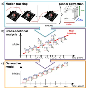
The proposed method makes use of the parameterisation proposed in [14] to describe the motion of each subject, and align spatially and temporally to a common reference frame for comparison (cf. Sec. II-A). The key novelty of this work is that these parameters are stacked to a tensor, which is pre-conditioned to center the data and ensure equal weighting of each parameter in the statistical analysis, as described in Sec. III-A1. We propose to perform cross-section analysis of the resulting tensors, as described in Sec. III-B. The proposed method for computing the motion parameters based on input age values is described in Sec. III-C. The proposed pipeline is summarised in Fig. 1.
P4
Mean
trajectory
Motion tracking Tensor Extraction
Cross-sectional analysis Motion Generative model Motion Time a) b) c) (years) (years)
Fig. 1: Proposed pipeline to build a generative model of the long-term motion changes in a population (c) by a) building a data tensor of polyaffine motion parameters that represent the motion over the cardiac cycle for each subject in the population using cross-sectional statistical analysis of polyaffine tensors and b) performing cross-sectional statistical analysis of the data tensors.
A. Testing Data-set
The proposed methods were applied to the polyaffine pa-rameters computed in [14]. These papa-rameters were found to yield results with a level of accuracy equivalent to state-of-the-art methods for cine-CMR tracking of the left ventricle of the heart. The data-set consists of two populations: the first a control group of 15 healthy volunteer adults (3 female, mean age ± SD = 28 ± 5), the second consisting of a group of 10 patients with repaired Tetralogy of Fallot (5 female, mean age ± SD = 15 ± 6). Details on the image data can be found in [14].
1) Data Centering and Scaling: An important factor in statistical analysis is the pre-conditioning of the data [41]. Ideally, the data should be centered with respect to the mean, and there should be no large differences between the scaling of one parameter and the scaling of another. Therefore, centering and scaling of the data should be carried out before performing the model calibration. In the case of matrices, the centering can be performed by computing the mean over all the observations and removing this mean from each observation.
Scaling the data can be more challenging when there are some meaningful scaling in the data that needs to be retained. When the data has some spatial and temporal components, as is often the case in motion tracking, these should not be uniformly scaled since the important spatial and temporal factors will thus be scaled out. With the parameterisation of the motion used in this work, the affine parameters need to be scaled since the affine (shear, rotation, scale) parameters may have very different scales to the translation parameters. Scaling the affine and translation parameters while retaining the meaningful differences between the spatial and temporal components is challenging when the data tensor is matricised. On the other hand, when the data structure is maintained, scaling along only one mode (direction) of the data tensor with the N-way PLS method is straightforward [41].
B. Dynamic Evolution Modelling
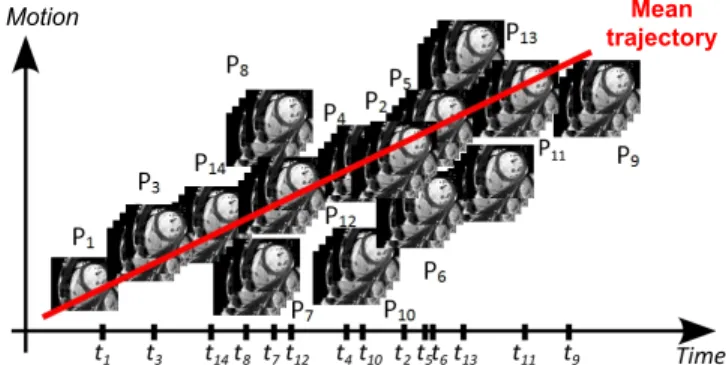
Inspired by the approach described in [22] to model the shape (i.e. static observations) from different subjects at dif-ferent stages of the evolution (c.f Sec. II-B), we propose to derive a dynamic growth model. Rather than regressing the static observations, we instead apply cross-sectional analy-sis to transformations computed over the cardiac cycle for each subject, as shown in Fig. 2. In [22], the deformations were those obtained by an LDDMM based registration [42]. The motion model described in [14] rather uses Polyaffine transformations. As described in [14], the mean motion of a population is estimated by averaging the motion of a set of subjects, which in this case involves the averaging the Polyaffine transformations after spatio-temporal realignment. Since the transformations of the mean motion model and the subject-specific motion models are described by regional affine matrices, computing the deviation of each subject from the mean requires simple matrix subtraction. As with the static growth model, the variation around the mean is computed using PLS to obtain factors most related to growth.
C. Computing Motion at Given Ages
Given the large number of parameters compared to the number of observations, N-way PLS is applied to generate a model for Y (age) given X (motion). However, we are interested in computing motion at given ages. The reversion of the computation was performed in [22] by using CCA to compute the regression coefficients for computing Y (in their case, body surface area) from X (in their case, shape), as mentioned in Sec. II-B. We propose to instead use the NIPALS formulation directly to reverse the direction of computation.
Motion Mean
trajectory
Fig. 2: Linear cross-sectional analysis is applied to motion transformations to regress the motion of a set of patients at different stages in the progression of the disease.
The computed model from the NIPALS method (and equiv-alently the N-way PLS method) computes the matrix D, as given in Eq. 11, which relates Y to X. More precisely, D models the relationship between the latent variables describing X and Y . Following the same method to derive the model of Y given in Eq. 12, a model of X can be derived by rearranging Eq. 11 for T as
T = U D0− HD0, (13)
which uses the fact that T and U are orthonormal, so that D
is then also orthonormal: D−1 = (T0U )−1 = U−1T0−1 =
U0T = D0. Replacing T in Eq. 3 with T from Eq. 13:
Xtest = T P0+ E (14)
= (U D0− HD0)P0+ E
= U D0P0+ E∗,
where E∗ = HD0P0+ E. Again, we assume that the latent
variable representations of X and Y fully capture X and Y ,
so that the residuals H and E are zero, and thus E∗ is zero.
So, using U from Eq. 7, the final model for X can be written as a linear regression model as:
Xtest = YtestB,˜ (15)
where ˜B = CD0P0 is the new matrix of regression
coeffi-cients, and C was defined in Eq. 9.
Note that this formulation for X is an approximation only since the latent variables are not computed in a symmetric manner as in PCA, i.e. T and U are computed to maximise the covariance between X and Y . However, we would ideally like
to have an equivalent formulation where T = U ˜D to compute
a new diagonal matrix ˜D. This detail is important due to the
iterative nature of all PLS algorithms, where U is initialised first, then T is computed. If both U and T are computed in parallel then this is not an important detail. An alternative option in the case where a large dataset is available (i.e. more observations than motion parameters), it may be possible to compute motion from age directly by setting X as the age and Y as the motion parameters.
IV. EXPERIMENTS
In order to analyse the proposed framework and different methods, two sets of experiments were performed. Firstly, a
quantitative analysis of the different methods by comparing the accuracy of estimating the output variable (age) given the input variables (the motion parameters) was performed. For the clinical example used in this work, such an estimation has little clinical value since the age of a patient is known a priori. Furthermore, previous work has already addressed this task, such as in [16]. Nonetheless, for comparative purposes this provides a way to quantitatively assess the potential of using such methods to relate motion parameters to age, and then to compare different algorithms in terms of the number of parameters and the degree of accuracy of each method.
The second set of experiments performed in this work was an assessment of the estimation of the input variables given the output variables, to assess the feasibility of computing full motion dynamics from age alone (i.e. can we obtain physiologically realistic motion dynamics). For the described clinical example, only qualitative assessment was performed due to the lack of longitudinal clinical data available (i.e. no long-term follow-up data), and because quantitative (e.g. voxel-wise) validation of the motion evolution model would require a model that couples the motion with structure, since structural remodelling that occurs over time in diseased pa-tients will result in a resampling of the voxels in the patient images over time. Voxel-wise quantification of the motion would assume that no structural remodelling occurs over time in these patients, and since this is not a valid assumption for these patients, no such validation is performed in this work.
A. Quantitative Comparison of Different Methods
Leave-one-out cross-validation was performed to assess the accuracy of the different methods for estimating age given the motion parameters. A leave-one-out design was chosen given the small data-set used in this work, to maximise the number of samples used in the training set.
The ToF population was chosen for these experiments given that there are more pronounced differences in motion for the different ages, whereas in contrast, motion in a healthy population should remain stable over time. We are interested in motion information related to age rather than total motion variability, and therefore the amount of variability describing the output variable age (Y ) is important, rather that the percentage of variability describing the input variables in the motion parameters X.
All experiments were carried out in Matlab R2012b using openly available Matlab codes for the N-way toolbox [43]. Nonlinear terms were computed with a built-in Matlab func-tion (x2fx.m). In all experiments, the data was pre-centered and pre-scaled (when scaling was applied). All leave-one-out errors are values for the error of the estimation of Y (age), and are thus expressed in years. Following the same analysis as in [22], the “one standard error” rule of thumb [44] is used, where errors less than one standard error of age are considered to be reasonable. The optimal method for this application is considered to be one which provides a suitable trade-off between accuracy and the number of parameters, since fewer parameters improves robustness and reproducibility.
1) Comparing Higher-Order Tensor and Matrix Analysis: In order to retain the structure of the data in X, tensor decomposition was compared to decomposition of the un-folded tensor, where the unfolding was done by concatenating the variables of the different modes into a 2-way matrix. The N-way PLS method was applied to the 4-way tensor of parameters stacked by affine parameters, region, and time for all subjects. Using this method, 4 components were needed to capture 98% of the shape variability, compared to 3 components for the matrix decomposition. The leave-one-out error (in years) in the tensor case was 4.34years, compared to 3.68years for the matrix decomposition. The amount of parameters required in the tensor decomposition was 232 (= 4 × 12 + 4 × 17 + 4 × 29), compared to 17748 for the matrix decomposition. Going from matrix analysis to tensor analysis results in a significant reduction in the number of parameters required to represent the motion. In these experiments the tensor analysis comes at the cost of a mild increase to the error, compared to the matrix analysis.
2) The Effect of Scaling: Scaling was applied on the affine
parameters in order to account for the fact that the affine pa-rameters can differ significantly in terms of scale, particularly between the translation components and the remaining affine components. The regional (spatial) and temporal axes of the tensor were left unscaled to retain the important differences in timing and region. The number of components required to capture 98% of the variability with scaling was the same as the number of components without scaling, and thus the number of parameters for each model were also the same (4 modes, 232 parameters). The leave-one-out error with scaling was lower than without scaling: 3.91years compared to 4.50years.
3) Incorporating Nonlinear Terms: To test whether
in-cluding nonlinear terms would improve the prediction ac-curacy, decomposition was applied to 5-way arrays of X
(10 × 12 × 17 × 29 × 1), [X; X2] (10 × 12 × 17 × 29 × 2),
[X; sin(X); cos(X)] (10 × 12 × 17 × 29 × 3), and [X; X2;
sin(X); sin(X2); cos(X); cos(X2)] (10 × 12 × 17 × 29 × 6).
The leave-one-out error results and number of components and parameters for each decomposition are summarised in Fig. 4. All decompositions were applied using N-way PLS with scaling on the affine parameters, given that this configuration gave the best results from the linear experiments. The optimal
results were found for [X; X2; sin(X); sin(X2); cos(X);
cos(X2)], with a leave-one-out error of 3.66years.
4) Visual Comparison of Different Methods: To visually
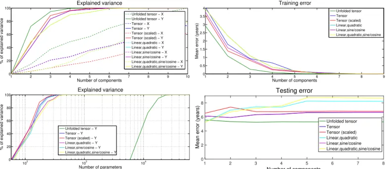
compare the different methods, a number of plots are pre-sented. Firstly, the percentage of variance explained in motion parameters (X) and age (Y ) for each method is shown in Fig. 3, as a function of the number of components in each decomposition. The variance explained in motion rises quicker for the nonlinear decompositions than with the linear compositions, however, the reverse is true for the variance explained in age. Since we are more interested in the variance of age than the variance of the motion parameters, this suggests that the linear models are more appropriate since they can capture the variance of age with fewer components (and thus fewer parameters).
1 2 3 4 5 6 7 8 9 10 0 20 40 60 80 100 Number of components % of explained variance Explained variance Unfolded tensor − X Unfolded tensor − Y Tensor − X Tensor − Y Tensor (scaled) − X Tensor (scaled) − Y Linear,quadratic − X Linear,quadratic − Y Linear,sine/cosine − X Linear,sine/cosine − Y Linear,quadratic,sine/cosine − X Linear,quadratic,sine/cosine − Y 102 103 104 0 20 40 60 80 100 Number of parameters % of explained variance Explained variance Unfolded tensor − Y Tensor − Y Tensor (scaled) − Y Linear,quadratic − Y Linear,sine/cosine − Y Linear,quadratic,sine/cosine − Y
Fig. 3: Percentage of variance explained in motion parameters (X) and age (Y ) for the linear models (left) and comparing the respective number of parameters between matrix and tensor methods (right). Tensor methods capture the variance in Y with significantly fewer parameters since the number of parameters equals the number of components N × (number of affine parameters + number of regions + number of time frames) (= 12 + 17 + 29), whereas the matrix methods result in N × (12 × 17 × 29).
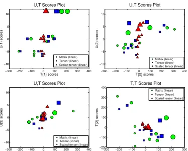
methods, the U, T plots for the first three components, and the
T, T score plot of T1vs. T2are shown in Fig. 5 for the matrix,
tensor, and scaled-tensor decompositions. The score plots in Fig. 5 show linear relationships between the latent variables in X and Y for the first and the third component, but some nonlinearities in the second component seem to be uncaptured by the models. The much clearer relationship in the T (1)-U (1)-plot than in the others is due to that the PLS algorithm always seeks to maximise the explained T -U covariance, and that the first PLS component is the linear combination of the original variables that explains the largest proportion of this covariance.
B. Clinical Application: Healthy vs. ToF Motion Evolution Given the low error of the linear N-way model with tensor pre-scaling, and that this configuration required the smallest number of parameters, this decomposition was used for the clinical analyses. For this decomposition applied to the control group, 7 components were required to capture 98% of the variability in age. The training error for this group was 0.48years, suggesting that this model fits the training set for the control population. The leave-one-out error of 3.95years was less than the population standard deviation for this group (5.0years). This model was found to be the most appropriate model for the ToF group (i.e. the model with the minimum number of components explaining a sufficient amount of the covariance), therefore, for the sake of comparison the same
1 2 3 4 5 6 7 8 9 0 0.5 1 1.5 2 2.5 3 3.5 4 Number of components
Mean error (years)
Training error Unfolded tensor Tensor Tensor (scaled) Linear,quadratic Linear,sine/cosine Linear,quadratic,sine/cosine 1 2 3 4 5 6 7 8 Number of components 0 2 4 6 8
Mean error (years)
Testing error Unfolded tensor Tensor Tensor (scaled) Linear,quadratic Linear,sine/cosine Linear,quadratic,sine/cosine
Fig. 4: Comparing the mean prediction error between N-way PLS applied to the unfolded tensor, full tensor with and without scaling, and the full tensor with quadratic and/or sine/cosine terms, for the training set (top) and cross-validation leave-one-out testing set (bottom) against the number of components. The unfolded tensor yielded the lowest testing error (5.24years), though the tensor with quadratic terms yielded similar accuracy (5.26years) with significantly fewer parameters (60 vs. 17748).
model was used for the control group.
Given the formulation of the proposed method, the affine, regional, and temporal parameters for each group can be directly compared. The first (log) affine component for the control population was:
M1controls = 0.0076 −0.0079 −0.015 0.63 −0.014 0.0035 0.0067 1.54 0.017 −0.0036 −0.0004 −2.12 ,
and for the ToF group:
MT oF 1 = 0.0018 −0.0031 0.0050 −1.07 −0.0062 −0.0026 −0.0041 2.27 0.0011 0.011 0.032 −3.43 .
The regional components can be visualised using the bulls-eye representation of the left ventricle proposed by the Amer-ican Heart Association [45]. The first component for each group is shown in Fig. 6, where each region is coloured according to the value for that region. These plots indicate that there is more homogeneous loadings for the control group compared to the ToF group, where the ToF group have larger values in the mid-septal regions and around the apex.
The first temporal component for each group is shown in Fig. 7. The temporal component for the control group follows similar trends to the typical volume curves found in healthy subjects (decreasing from the end-diastolic frame until the systolic frame, followed by an increase back to the end-diastolic frame). The ToF group shows a slower increase after
−300 −200 −100 0 100 200 300 400 −10 −5 0 5 10 T(1) scores U(1) scores
U,T Scores Plot
Matrix (linear) Tensor (linear) Scaled tensor (linear)
−300 −200 −100 0 100 200 300 400 −10 −5 0 5 10 T(2) scores U(2) scores
U,T Scores Plot
Matrix (linear) Tensor (linear) Scaled tensor (linear)
−300 −200 −100 0 100 200 300 400 −10 −5 0 5 10 T(3) scores U(3) scores
U,T Scores Plot
Matrix (linear) Tensor (linear) Scaled tensor (linear)
−300 −200 −100 0 100 200 300 −200 −100 0 100 200 300 400 T(1) scores T(2) scores T,T Scores Plot Matrix (linear) Tensor (linear) Scaled tensor (linear)
Fig. 5: Score plots for each of the linear NIPALS decomposi-tions (matrix shown with circles, unscaled tensor shown with squares, and scaled tensor shown with triangles) for U vs. T for the first components (top left), second components (top right), and third components (bottom left), and T vs T for the first two components (bottom right). The symbols are sized according to age (Y ).
-0.1 0.5
Controls
-0.1 0.5
ToF
Fig. 6: The first regional model from each population. The regional component for the control group shows more homo-geneous regional behaviour, in comparison to the ToF group, where there is larger values in the mid septal regions, and around the apex.
end-systole, compared to the control group, and does not come back to zero, suggesting some potential drift effects in this group. Note that the interpretation of the different factors (spatial, temporal, affine) was provided in previous work [46]. Given the formulation of the proposed method, cine se-quences can be regenerated from the models to visualise the cardiac motion at each age by applying Log-Euclidean Polyaffine Transformations computed from the predicted polyaffine parameters to a chosen reference image. Note that perceived motion outside of the AHA regions is the result of smoothing of the Gaussian weights and motion outside of the region of interest is not the intended focus of the generated images. Snapshots of the images at ±2 standard deviations
5 10 15 20 25 −0.5 −0.4 −0.3 −0.2 −0.1 0 0.1 Frame
First Temporal Component
Controls ToF
Fig. 7: The first temporal component from each population. The temporal component for the control group closely re-sembles the left ventricle volume curves observed in healthy subjects. The ToF components show less pronounced (slower) contraction and filling.
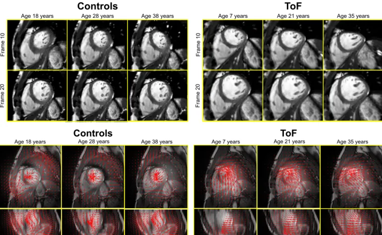
of the age (Y ) of each group, and at the mean age of each group are shown at frames 10 (end-systole) and 20 (end of relaxation) are shown in Fig. 8 (top) for the control group and in Fig. 9 (top) for the ToF group. The deformation fields at the end-systolic phase (frame 10) for each group are shown in Fig. 8 (bottom), at ±2 standard deviations of age, and at the mean age for the control group and Fig. 9 (bottom) for the ToF group. For the control group deformations, we see little changes in the overall dynamics.
V. DISCUSSION
In all of the numerical experiments (Sec. IV-A), the training error was very low for the linear models, indicating that the models were all able to fit the training sets well. In these experiments, the errors were compared to the stan-dard deviation in Y , using the “one stanstan-dard-error” rule of thumb, where we assume that the optimal model of Y is Y itself, and therefore one standard-error corresponds to one standard deviation [44]. With this criteria, all models were sufficiently accurate. Note that the NIPALS algorithm requires initialisation of the T scores from Eq. 3, which is performed internally using random values. This can affect the final leave-one-out errors, so in all cases where the NIPALS algorithm was used, 100 experiments were run to ensure that the leave-one-out errors were representative. Therefore, the presented leave-one-out errors are actually the average values of all 100 experiments. The mean standard deviation of all experiments was 0.007 for the training set, and 0.06 for the testing set, thus the method is reasonably insensitive to the initialisation. Looking at the results in more details, comparing tensor decomposition with matrix decomposition, the error of the tensor decomposition was slightly higher, however, the number of parameters required to model the data is significantly lower when retaining the tensor structure of the data. Thus, we believe that a small decrease in accuracy is acceptable given the large decrease in parameters required for the model. Furthermore, retaining the tensor structure allows pre-scaling to be performed on the affine parameters to ensure that the
Age 18 years Age 28 years Age 38 years
Frame 10
Frame 20
Controls
Age 18 years
Controls
Age 28 years Age 38 yearsFig. 8: Snapshots of the motion at ±2 standard deviations and at the mean for the control group (top) at frame 10 (corresponding to the end-systolic frame), and frame 20 (cor-responding to the end of relaxation) and the cor(cor-responding deformation fields (bottom).
translation components of the affine matrix are not weighted higher in the decomposition, which is often the case given the typically greater scale of these components. When pre-scaling is applied to the affine parameters, the error is lower than for the other methods, and requires the least number of param-eters to describe the model. Therefore, tensor decomposition with pre-scaling appears to be the optimal method for this dataset. Tensor decomposition with pre-scaling on the affine parameters was used for the nonlinear experiments given that this gave the lowest testing error. The nonlinear experiments suggest that the use of higher order and sine/cosine terms in the design matrix can improve the accuracy of the estimation. The use of quadratic terms in the design matrix can account for some nonlinearity in the data, and the sine and cosine terms can be used to model periodicity, which is relevant for this data since the motion parameters are periodic (they should start and finish at zero since cardiac motion is cyclic). The error is slightly lower when quadratic and sine/cosine terms are incorporated in the design matrix, at the expense of adding 24 parameters to the model.
In this work, nonlinearity was incorporated in the model by adding nonlinear features within the linear PLS framework. Nonlinearity can also be incorporated by using a neural network framework [47], using a fuzzy inference system [48],
Age 7 years Age 21 years Age 35 years
Frame 10
Frame 20
ToF
Age 7 years Age 21 years
ToF
Age 35 yearsFig. 9: Snapshots of the motion at ±2 standard deviations and at the mean for the ToF group (top) at frame 10 (corresponding to the end-systolic frame), and frame 20 (corresponding to the end of relaxation) and the corresponding deformation fields (bottom).
or by modelling the relationship between X and Y using a nonlinear function [49] or with splines [50]. The linear and nonlinear extensions used in this study were considered sufficient to model the available data, based on the training and testing errors. However, with more data, other nonlinear models will be further investigated. With a larger number of observations, hierarchical cluster-based PLS [51], [52] could be used to account for clustering in the data. This would be useful to, for example, account for differences following alternative treatment courses.
While this work was focussed on analysis of cardiac motion over time, the proposed methods could be used to model the evolution over time from any images (medical, media, security footage, etc.), where the changes over time are of interest. Polyaffine models are a useful extension of local affine, global affine, and rigid transformation model to capture more nonlinear transformations, without requiring many more degrees of freedom, as in nonrigid (i.e. elastic) transformation models.
A possible future improvement of this approach could be to account for e.g. gender and pathology (control vs. ToF) in addition to age to decrease the inter-subject variability and allow for a common model for the control and ToF groups.
Limitations: In all experiments, the number of observations is small, therefore it is difficult to draw a fully meaningful clinical conclusion from these experiments alone. In addi-tion, a comparison is made between PLS subspaces though these were computed on cohorts with different age ranges. Furthermore, while an advantage of the AHA division of seg-ments is the low number of regions leading to lower number of parameters. However, a possible limitation is that AHA segments are mostly suitable for ischemic events, therefore by limiting transformations to those segments it may not be possible to accurately characterize functional remodeling in other cardiovascular diseases such as ToF.
Another limitation of this study is that the use of a statistical model of cardiac function at different ages to analyse the evolution of the heart over time relies on the assumption that cohort effects reflect longitudinal effects. As shown in [53], this may not be a valid assumption. Hence, future validation of this approach by use of longitudinal data is needed in order to draw clinical conclusions.
In spite of these limitations, the results suggest that the proposed method is able to model changes in motion over time in a given population, and with larger datasets the error is expected to decrease since the estimation will become less sensitive to outliers. However, in absence of data to quantitatively validate the prediction of motion based on age, it is difficult to draw conclusions regarding the difference between the patient and their age-predicted motion as the observed differences could be due to, for example, different disease processes.
VI. CONCLUSION
The proposed method constitutes, to our knowledge, a first attempt to statistically model the evolution of cardiac motion over time for a given population. The method makes use of a recently developed method for describing and compar-ing cardiac motion within and across populations uscompar-ing a polyaffine model. The advantage of using a model to describe the motion is that the number of parameters remains low, while maintaining sufficient accuracy in the motion tracking (on a par with state-of-the-art cardiac motion tracking methods). Furthermore, the definition of the parameters is consistently defined from one subject to another, and following spatial and temporal alignment, can be quantitatively compared within and between populations. The novelty of the proposed method lies in taking advantage of this compact representation of motion and using statistical cross-sectional analysis of the motion parameters to compute the evolution over years of the motion observed within a given population. Analysis of higher-order data arrays was chosen to retain structuring of the motion data as well as for the advantage of obtaining components that can be more readily analysed and understood as their respective spatial, temporal, and affine components. The clinical advantage of such a method is that the knowledge of how the motion dynamics evolve in a specific population as a disease progresses can be used to guide therapy planning to optimise the timing and choice of intervention.
ACKNOWLEDGMENTS
This project was carried out as a part of the Centre for Cardiological Innovation (CCI), Norway, funded by the Re-search Council of Norway. The authors would like to thank Sandia National Laboratories for providing open source tools for tensor manipulation and decomposition (Tensor Toolbox, Matlab, Mathworks), and Claus Andersson and Rasmus Bro for providing open source tools for performing N-Way tensor manipulation (N-Way Tensor Toolbox, Matlab, Mathworks).
REFERENCES
[1] A. F. Frangi, W. J. Niessen, and M. A. Viergever, “Three-dimensional modeling for functional analysis of cardiac images, a review,” Medical Imaging, IEEE Transactions on, vol. 20, no. 1, pp. 2–5, 2001. [2] H. Wang and A. A. Amini, “Cardiac motion and deformation recovery
from MRI: a review,” Medical Imaging, IEEE Transactions on, vol. 31, no. 2, pp. 487–503, 2012.
[3] A. Suinesiaputra, P. Ablin, X. Alba et al., “Statistical shape modeling of the left ventricle: myocardial infarct classification challenge,” IEEE Journal of Biomedical and Health Informatics, vol. PP, no. 99, pp. 1–1, 2017.
[4] S. Ardekania, S. Jain, A. Sanzi et al., “Shape analysis of hypertrophic and hypertensive heart disease using mri-based 3d surface models of left ventricular geometry,” Medical Image Analysis, vol. 29, pp. 12–23, 2016.
[5] P. Medrano-Gracia, B. R. Cowan, A. Suinesiaputra, and A. A. Young, “Atlas-based anatomical modeling and analysis of heart disease,” Drug Discovery Today: Disease Models, vol. 14, pp. 33–39, 2014.
[6] L. Tautz, A. Hennemuth, and H.-O. Peitgen, “Motion analysis with quadrature filter based registration of tagged MRI sequences,” in Proc. STACOM MICCAI Workshop, ser. LNCS. Springer, 2011.
[7] T. Mansi, X. Pennec, M. Sermesant, H. Delingette, and N. Ayache, “iLogDemons: A demons-based registration algorithm for tracking in-compressible elastic biological tissues,” Int J. of Comp Vision, vol. 92, no. 1, pp. 92–111, 2011.
[8] R. Chandrashekara, R. Mohiaddin, and D. Rueckert, “Cardiac motion tracking in tagged MR images using a 4D B-spline motion model and nonrigid image registration,” in IEEE Int. Symp. on Biomed. Imaging: Nano to Macro, 2004, pp. 468–471.
[9] W. Shi, X. Zhuang, H. Wang, S. Duckett, D. V. Luong, C. Tobon-Gomez, K. Tung, P. J. Edwards, K. S. Rhode, R. S. Razavi et al., “A comprehensive cardiac motion estimation framework using both untagged and 3D tagged MR images based on nonrigid registration,” IEEE Trans. Med. Imaging, vol. 31, no. 6, pp. 1263–1275, 2012. [10] B. Heyde, D. Barbosa, P. Claus, F. Maes, and J. D’hooge,
“Three-dimensional cardiac motion estimation based on non-rigid image reg-istration using a novel transformation model adapted to the heart,” in Proc. STACOM MICCAI Workshop, ser. LNCS, 2012.
[11] M. De-Craene, C. Tobon-Gomez, C. Butakoff, N. Duchateau, G. Piella, K. Rhode, and A. Frangi, “Temporal diffeomorphic free form defor-mation (TDFFD) applied to motion and defordefor-mation quantification of tagged MRI sequences,” in Proc. STACOM MICCAI Workshop, ser. LNCS. Springer, 2011.
[12] W. Zhang, J. Noble, and J. Brady, “Spatio-temporal registration of real time 3D ultrasound to cardiovascular MR sequences,” Medical Image Computing and Computer-Assisted Intervention–MICCAI 2007, pp. 343–350, 2007.
[13] M. S. Hansen, S. S. Thorup, and S. K. Warfield, “Polyaffine parametriza-tion of image registraparametriza-tion based on geodesic flows,” in Proc. MMBIA Workshop. IEEE, 2012, pp. 289–295.
[14] K. McLeod, M. Sermesant, P. Beerbaum, and X. Pennec, “Spatio-temporal tensor decomposition of a polyaffine motion model for a better analysis of pathological left ventricular dynamics,” IEEE Transactions on Medical Imaging, 2015.
[15] K. Mcleod, M. Sermesant, P. Beerbaum, and X. Pennec, “Descriptive and intuitive population-based cardiac motion analysis via sparsity constrained tensor decomposition,” in Medical Image Computing and Computer-Assisted Intervention–MICCAI 2015. Springer, 2015, pp. 419–426.
[16] W. Bai, D. Peressutti, O. Oktay, W. Shi, D. P. ORegan, A. P. King, and D. Rueckert, “Learning a global descriptor of cardiac motion from a large cohort of 1000+ normal subjects,” in International Conference on Functional Imaging and Modeling of the Heart. Springer, 2015, pp. 3–11.
[17] T. Kuznetsova, L. Thijs, J. Knez, N. Cauwenberghs, T. Petit, Y.-M. Gu, Z. Zhang, and J. A. Staessen, “Longitudinal changes in left ventricular diastolic function in a general population,” Circulation: Cardiovascular Imaging, vol. 8, no. 4, p. e002882, 2015.
[18] O. Savu, R. Jurcut, S. Giusca, T. Van Mieghem, I. Gussi, B. A. Popescu, C. Ginghina, F. Rademakers, J. Deprest, and J.-U. Voigt, “Morphological and functional adaptation of the maternal heart during pregnancy,” Circulation: Cardiovascular Imaging, pp. CIRCIMAGING–111, 2012. [19] A. Hallbergson, K. Gauvreau, A. J. Powell, and T. Geva, “Right
ventricular remodeling after pulmonary valve replacement: Early gains, late losses,” The Annals of thoracic surgery, vol. 99, no. 2, pp. 660–666, 2015.
[20] G. E. Assenza, D. Cassater, M. Landzberg, T. Geva, J. Schreier, D. Graham, M. Volpe, N. Barker, K. Economy, and A. M. Valente, “The effects of pregnancy on right ventricular remodeling in women with repaired tetralogy of fallot,” International journal of cardiology, vol. 168, no. 3, pp. 1847–1852, 2013.
[21] J. A. Cuypers, M. E. Menting, E. E. Konings, P. Opi´c, E. M. Utens, W. A. Helbing, M. Witsenburg, A. E. van den Bosch, M. Ouhlous, R. T. van Domburg et al., “The unnatural history of tetralogy of fallot: prospective follow-up of 40 years after surgical correction,” Circulation, pp. CIRCULATIONAHA–114, 2014.
[22] T. Mansi, I. Voigt, B. Leonardi, X. Pennec, S. Durrleman, M. Sermesant, H. Delingette, A. M. Taylor, Y. Boudjemline, G. Pongiglione, and N. Ay-ache, “A statistical model for quantification and prediction of cardiac remodelling: Application to tetralogy of fallot,” IEEE Transactions on Medical Imaging, vol. 9, no. 30, pp. 1605–1616, Sep. 2011.
[23] K. McLeod, M. Sermesant, and X. Pennec, “Improving understanding of long-term cardiac functional remodelling via cross-sectional analysis of polyaffine motion parameters,” in International Conference on Func-tional Imaging and Modeling of the Heart. Springer, 2017, pp. 51–59. [24] N. Ablitt, J. Gao, J. Keegan, L. Stegger, D. N. Firmin, G.-Z. Yang et al., “Predictive cardiac motion modeling and correction with partial least squares regression,” Medical Imaging, IEEE Transactions on, vol. 23, no. 10, pp. 1315–1324, 2004.
[25] K. Lekadir, X. Alb`a, M. Perea˜nez, and A. F. Frangi, “Statistical shape modeling using partial least squares: Application to the assessment of myocardial infarction,” in Statistical Atlases and Computational Models of the Heart. Imaging and Modelling Challenges. Springer, 2015, pp. 130–139.
[26] J. L. Bruse, K. Mcleod, G. Biglino, H. N. Ntsinjana, C. Capelli, T.-Y. Hsia, M. Sermesant, X. Pennec, A. M. Taylor, and S. Schievano, “A non-parametric statistical shape model for assessment of the surgically repaired aortic arch in coarctation of the aorta: How normal is abnor-mal?” in Statistical Atlases and Computational Models of the Heart. Imaging and Modelling Challenges. Springer, 2015, pp. 21–29. [27] Y. Yu, J. Jin, F. Liu, and S. Crozier, “Multidimensional compressed
sensing mri using tensor decomposition-based sparsifying transform,” 2014.
[28] R. Bro, “Multiway calidration. multilinear pls,” Journal of chemometrics, vol. 10, pp. 47–61, 1996.
[29] O. Commowick, V. Arsigny, A. Isambert, J. Costa, F. Dhermain, F. Bidault, P.-Y. Bondiau, N. Ayache, and G. Malandain, “An efficient locally affine framework for the smooth registration of anatomical structures,” Med. Image Anal., vol. 12, no. 4, pp. 427–441, 2008. [30] V. Arsigny, O. Commowick, N. Ayache, and X. Pennec, “A fast and
log-euclidean polyaffine framework for locally linear registration,” J. of Math. Imaging and Vision, vol. 33, no. 2, 2009.
[31] C. Seiler, X. Pennec, and M. Reyes, “Capturing the multiscale anatom-ical shape variability with polyaffine transformation trees,” Med. Image Anal., pp. 1371–1384, 2012.
[32] K. McLeod, C. Seiler, M. Sermesant, and X. Pennec, “A near-incompressible poly-affine motion model for cardiac function analysis,” in Proc. STACOM MICCAI Workshop, ser. LNCS. Springer, 2012. [33] K. Mcleod, C. Seiler, N. Toussaint, M. Sermesant, and X. Pennec,
“Regional analysis of left ventricle function using a cardiac-specific polyaffine motion model,” in Proc. FIMH’13, 2013, pp. 483–490. [34] N. Toussaint, C. T. Stoeck, T. Schaeffter, S. Kozerke, M. Sermesant,
and P. G. Batchelor, “In vivo human cardiac fibre architecture estimation using shape-based diffusion tensor processing,” Medical Image Analysis, pp. 1243–1255, 2013.
[35] W. Bai, W. Shi, A. de Marvao, T. J. Dawes, D. P. ORegan, S. A. Cook, and D. Rueckert, “A bi-ventricular cardiac atlas built from 1000+ high resolution mr images of healthy subjects and an analysis of shape and motion,” Medical image analysis, vol. 26, no. 1, pp. 133–145, 2015. [36] M. Lorenzi and X. Pennec, “Efficient parallel transport of deformations
in time series of images: from schilds to pole ladder,” Journal of mathematical imaging and vision, vol. 50, no. 1-2, pp. 5–17, 2014. [37] P. Geladi and B. R. Kowalski, “Partial least-squares regression: a
tutorial,” Analytica chimica acta, vol. 185, pp. 1–17, 1986.
[38] R. Rosipal and N. Kr¨amer, “Overview and recent advances in partial least squares,” in Subspace, latent structure and feature selection. Springer, 2006, pp. 34–51.
[39] H. Wold et al., “Estimation of principal components and related models by iterative least squares,” Multivariate analysis, vol. 1, pp. 391–420, 1966.
[40] S. De Jong, “Simpls: an alternative approach to partial least squares regression,” Chemometrics and intelligent laboratory systems, vol. 18, no. 3, pp. 251–263, 1993.
[41] R. Bro and A. K. Smilde, “Centering and scaling in component analysis,” Journal of Chemometrics, vol. 17, no. 1, pp. 16–33, 2003.
[42] S. Durrleman, X. Pennec, A. Trouv´e, and N. Ayache, “Statistical models on sets of curves and surfaces based on currents,” Medical Image Analysis, vol. 13, no. 5, pp. 793–808, 2009.
[43] C. A. Andersson and R. Bro, “The n-way toolbox for matlab,” Chemo-metrics and Intelligent Laboratory Systems, vol. 52, no. 1, pp. 1–4, 2000.
[44] T. Hastie, R. Tibshirani, J. Friedman, and J. Franklin, “The elements of statistical learning: data mining, inference and prediction,” The Mathematical Intelligencer, vol. 27, no. 2, pp. 83–85, 2005.
[45] M. Cerqueira, N. Weissman, V. Dilsizian, A. Jacobs, S. Kaul, W. Laskey, D. Pennell, J. Rumberger, T. Ryan, and M. Verani, “Standardized myocardial segmentation and nomenclature for tomographic imaging of the heart,” Circulation, vol. 105, 2002.
[46] K. Mcleod, C. Seiler, M. Sermesant, and X. Pennec, “Spatio-temporal dimension reduction of cardiac motion for group-wise analysis and sta-tistical testing,” in MICCAI - Medical Image Computing and Computer Assisted Intervention - 2013, ser. Lecture Notes in Computer Science. Springer, Heidelberg, 2013.
[47] S. J. Qin and T. J. McAvoy, “Nonlinear pls modeling using neural networks,” Computers & Chemical Engineering, vol. 16, no. 4, pp. 379– 391, 1992.
[48] Y. H. Bang, C. K. Yoo, and I.-B. Lee, “Nonlinear pls modeling with fuzzy inference system,” Chemometrics and intelligent laboratory systems, vol. 64, no. 2, pp. 137–155, 2002.
[49] I. E. Frank, “A nonlinear pls model,” Chemometrics and intelligent laboratory systems, vol. 8, no. 2, pp. 109–119, 1990.
[50] S. Wold, “Nonlinear partial least squares modelling ii. spline inner relation,” Chemometrics and Intelligent Laboratory Systems, vol. 14, no. 1, pp. 71–84, 1992.
[51] K. Tøndel, U. G. Indahl, A. B. Gjuvsland, J. O. Vik, P. Hunter, S. W. Omholt, and H. Martens, “Hierarchical cluster-based partial least squares regression (hc-plsr) is an efficient tool for metamodelling of nonlinear dynamic models,” BMC systems biology, vol. 5, no. 1, p. 90, 2011. [52] K. Tøndel, U. G. Indahl, A. B. Gjuvsland, S. W. Omholt, and H. Martens,
“Multi-way metamodelling facilitates insight into the complex input-output maps of nonlinear dynamic models,” BMC systems biology, vol. 6, no. 1, p. 88, 2012.
[53] J. Eng, R. L. McClelland, A. S. Gomes et al., “Adverse left ventricular remodeling and age assessed with cardiac mr imaging: The multi-ethnic study of atherosclerosis,” Radiology, vol. 278, p. 714722, 2016.