HAL Id: halshs-00155739
https://halshs.archives-ouvertes.fr/halshs-00155739
Submitted on 23 Jul 2018HAL is a multi-disciplinary open access
archive for the deposit and dissemination of sci-entific research documents, whether they are pub-lished or not. The documents may come from teaching and research institutions in France or
L’archive ouverte pluridisciplinaire HAL, est destinée au dépôt et à la diffusion de documents scientifiques de niveau recherche, publiés ou non, émanant des établissements d’enseignement et de recherche français ou étrangers, des laboratoires
analysis with flexible prices and increasing returns
Gaël Giraud, Céline Rochon
To cite this version:
Gaël Giraud, Céline Rochon. Natural rate of unemployment and efficiency: a dynamic analysis with flexible prices and increasing returns. 2007. �halshs-00155739�
Centre d’Economie de la Sorbonne
Natural rate of unemployment and efficiency : a dynamic analysis with flexible prices and increasing returns
Gaël GIRAUD, CélineROCHON
A dynamic analysis with flexible prices and
increasing returns
Ga¨el Giraud
CNRS, Paris School of Economics
and
C´eline Rochon
Sa¨ıd Business School, University of Oxford
∗Abstract.— We present a continuous time non tˆatonnement process for fric-tionless and perfectly competitive markets with (possibly non convex) production, where the natural rate of unemployment (NRU) emerges as the asymptotic value of unemployment. Consumers and producers are myopic and repeatedly partici-pate in Mertens’(2003) limit-price mechanism. We show that underemployment and unsold inventories can survive along the solution paths of our dynamics—the hallmark of the failure of Say’s law. The following paradox appears: A nonzero NRU is compatible with Pareto optimality; conversely, full employment is com-patible with sub optimality. Nevertheless, each trade and production path of our price quantity dynamics converges to some infinitesimal Pareto optimal point as long as there are no unsold inventories at the limit.
Keywords. Underemployment, Say’s law, inventories, non convex produc-tion.
JEL Classification. D11, D21, D51, E24.
1
Introduction
This paper arises from two motivations. First, the traditional conclusions of the “fixed price” equilibrium approach developed in the 1970s were largely correct,
∗We wish to thank Professors Jean-Marc Bonnisseau, Bernard Cornet, Rodolphe Dos Santos
but they were not explored further because they failed to provide a theoretical explanation for price rigidities. Conversely, flexible-price equilibrium theory faces a basic stumbling block: How can underemployment emerge in a world where all markets are supposed to clear instantaneously ? Here we offer a paradigm where frictionless economies with perfectly flexible prices and wages exhibit Classical as well as Keynesian underemployment.
Second, standard theories of the natural rate of unemployment (NRU) are typically unable to draw any relationship between the equilibrium level of unem-ployment and the Pareto optimal level. Here, we provide a dynamic setup where the NRU can be thought of as the value to which the rate of unemployment converges as time goes to infinity and where efficiency properties of NRU can be tackled.
Let us look at these two issues in more detail. The fixed price equilibrium approach was based on the work by Barro and Grossman (1971), B´enassy (1973), Dr`eze (1975) and others1; in essence, it consisted of allowing prices to differ
from the flexible-price Walrasian equilibrium vector. Output in each market was then assumed equal to the minimum of supply and demand. According to this approach, if prices lead to excess supply in both goods and labor markets, as in Keynesian models, then firms are rationed in the goods markets so that the demand for labor is determined by output. The economy exhibits a demand multiplier: An increase in the demand leads to an increase in production, an increase in income, and further increases in the demand, and so forth. Excess demand in all markets yields a supply multiplier: Labor supply decreases and output decreases, which leads to further rationing in the goods market.
As a consequence, Blanchard (2000) notes that, without a theory of why prices differ from equilibrium prices, both outcomes (excess supply and excess demand on all markets) are equally probable. A theory of price setting is there-fore required. Furthermore, as observed by Roberts (1987), in the early models of disequilibrium theory, at least some prices or wages are exogenously fixed at levels that are not market clearing, and the models offer no basis for analysis of the opportunities for changing prices or of the incentives to do so. Some of them even assume that there is some unmodeled mechanism at work that ensures the maximum level of transactions consistent with voluntary exchange at the fixed prices and feasibility. In this paper, prices are flexible and are determined instan-taneously by a double auction, Mertens’ (2003) limit-price mechanism. Out of equilibrium, this mechanism provides a natural rationing rule akin to the short-side rule but much closer to actual trading institutions used in contemporary markets. Yet we exhibit both Keynesian and Classical underemployment as well as contained inflation. Moreover, the micro-structure being analyzed as a strate-gic market game, we specifically address the issue of stratestrate-gic incentives to change disequilibrium prices. Finally, the determination of quantities is made explicit and is also strategically chosen by players.
The main reason for the appearance of unemployment in our model is the pos-tulated bounded rationality of economic agents. More specifically, we assume that all of them are myopic. On the consumption side, myopia is captured by assuming that workers instantaneously maximize the (linear) first-order approximation of their current utility. This conforms to a well-established way of modeling myopia in non tˆatonnement models.2 As a consequence, each worker behaves in the short
run as if there were some reservation wage below which he refuses to work and at which his labor supply is vertical. On the production side, firms are myopic and instantaneously maximize their short run profit with respect to the (constant re-turn) first-order approximation of their production function. Thus, they behave as if they had some reservation wage above which they refuse to hire and at which their labor demand is vertical. We show that both effects, when combined with a second ingredient detailed below, generate underemployment along trajectories that are solutions to our dynamics.
Our second ingredient is a reinterpretation of production sets in a dynamic perspective. To grasp the intuition behind this new point of view, consider the simplest possible example of an economy with one producer and one consumer. Suppose the producer’s production set, Yj, exhibits strictly decreasing returns so
that, at a non trivial (standard) Walras equilibrium, this producer will have a positive profit, while the final production plan yj will be located somewhere on
the boundary ∂Yj of the production set Yj. Here, we question the logic behind
this familiar picture, as the following remarks indicate:
1) First, actually, production takes time, so that, before reaching yj, the
pro-ducer must have produced say 1 2yj,
3
4yj,... A little reflection suggests that, if each
partial production plan is to be feasible and efficient, then the producer’s plan should have evolved along the boundary ∂Yj from 0 (no production) to yj. In this
paper, we provide a formalization of this intuitive dynamics which remains hidden in static equilibrium theory, and we show that it can be extended to non-convex production.
2) Second, in static equilibrium theory, the unique shareholder of the firm, the consumer, receives the whole profit as dividend. At a standard Arrow Debreu equilibrium, this additional income instantaneously enters into the consumer’s budget and hence is used to finance the demand that is addressed to the unique firm. In this sense, Say’s law is automatically satisfied but at the cost of a vicious circle: The redistributed profit is supposed to finance the demand that is respon-sible for this very profit. One interpretation of this paradox is to say that the consumer can take short positions during the production process: What actually happens is that he borrows (at zero cost) a certain amount of cash in order to finance his purchases; these purchases induce some profits that are afterwards redistributed to the same consumer at the end of the day; in equilibrium, nobody remains in the red because the dividends exactly compensate the consumer’s loans.
2Smale (1976), Champsaur and Cornet (1990), Bottazi (1994), Bonnisseau and Florig (2003),
By contrast, in the situation we examine here, the output y+
j (t) produced at
time t by means of input yj−(t) cannot be put up for sale on commodity markets at time t, but only at t + dt. Because it is not available at t, y+
j (t) cannot be used
to finance the input y−
j (t) from which it is supposed to be produced (again,
“pro-duction takes time”). As a consequence, when buying consumption commodities, the consumer must be able to finance his purchases with the revenues from his current sales, not with the revenues of his future dividends.3 Since the
mecha-nism used to implement trades is balanced, the value of the firm’s sales must be equal to that of the household’s wage. It should thus come as no surprise that, at market-clearing prices, firms’ profits are always zero. We view this property as a virtue because increasing returns are known to generate negative profits at static marginal cost equilibria (Cornet 1988).4 As a result, in this paper, Walras’
law is always satisfied, but Say’s law is not; underemployment can appear on the labor market as well as unsold inventories on the commodity market; firms’ profits are constantly equal to zero and, whether convex or not, none of them ever goes bankrupt.
Roberts (1987) also provides an equilibrium model with unemployment at flexible, competitive prices and wages. There, however, imperfect competition is assumed and permits to generate a continuum of equilibria; all but the Walrasian ones involve inefficiently low levels of activity. Here, by contrast, perfect compe-tition is assumed throughout and captured by means of a continuum of negligible agents. In the present model, unemployment is not the consequence of infor-mational asymmetries as in works based on efficiency wage models (Shapiro and Stiglitz 1984). Here, indeed, there are no problems of hidden knowledge or un-observable actions. Finally, unlike in the Clower-Leijonhufvud interpretations of Keynes’ chap. 2 of the General Theory (Ito 1979), unemployment is not the result of self-enforcing pessimism about demand, as firms do not make any conjectures about demand. The very simplistic way we capture myopia enables therefore to focus on one aspect, apparently neglected so far: the fact that markets populated by boundedly rational players are consistent both with full employment and with inefficient, “recessionary” unemployment.
Once it was realized that “fixed price” equilibrium theory, in its present form, leads to dead ends, many market imperfections have been extensively studied since the 1980s — for example, price staggering (Taylor 1988) and labor search and bargaining (Diamond 1982b; Mortensen 1982; Pissarides 1985, 1999, to name but a few seminal papers). All these approaches, in a sense, add some kind of “viscosity” to the basic equilibrating mechanism that leads to market clearing. This viscosity, in turn, is responsible for the appearance of unemployment. Such
3This is consistent with the fact that, in “real life”, even so-called short sales are accompanied
by a private loan or repurchase contract. Following Mertens (2003, n. 3) we leave this aspect outside of the anonymous market by forbidding short sales.
4The introduction of fiat money (in the same vein as in Giraud and Tsomocos 2006) and of
a banking system will allow firms’ to make positive profits along trade-and-production paths. This is left for further research.
imperfections are compatible with our paradigm, and their impact will be ana-lyzed in subsequent work. The strength of our approach, however, is that we do not require them in order to exhibit underemployment, nor to state which type of underemployment will emerge. We show indeed that Classical underemployment and contained inflation should occur essentially when the short run (or “mar-ginal”) rate of substitution (to be defined in subsection 2.2) of the representative consumer exceeds the short run (or “marginal”) productivity of labor (see also subsection 2.2). Conversely, Keynesian underemployment is a consequence of the fact that the marginal rate of substitution is less than the marginal productivity of labor.
The second aspect of our contribution regards the relationships between un-deremployment and efficiency. The literature devoted to search and bargaining in a decentralized labor market usually leads to the conclusion that there will always be some unemployment and, moreover, that a very low rate of unem-ployment should be inefficient.5 However, as noted in Blanchard (2000), no such
theory provides a clear-cut relationship between unemployment and efficiency. Because, in this paper, the NRU does not depend upon issues of matching but only on the fundamental characteristics of the economy (agents’ short run preferences and firms’ short run productivity), efficiency issues can be formally explored. To be more precise, we prove that, provided there are no unsold in-ventories at the limit, every trade and production path converges towards some infinitesimal price equilibrium, hence to a locally optimal rest point. Moreover, we show by means of examples that a positive NRU is compatible with the re-silience of unsold inventories, hence with optimality as well as with suboptimality. Perhaps even more surprisingly, the same holds for a zero NRU: A solution path may converge towards a price equilibrium with full employment, which remains nevertheless suboptimal (because of the persistence of unsold inventories).
There is a reason why this puzzling lack of correspondence between optimality and full employment has not been discovered earlier: macroeconomic markets of Keynesian inspiration (where unemployment emerges) are usually stated within a representative agent model, where welfare issues cannot be addressed. Con-versely, general equilibrium models with heterogeneous agents do not permit one to analyze underemployment because, in such models, market clearing implies Say’s law. In this paper, we maintain market clearing throughout together with heterogeneous agents, but in a way that no longer automatically implies Say’s law.
The paper proceeds as follows. Section 2 sets-up our dynamics, emphasiz-ing the reinterpretation of production sets—on which our whole approach rests. Trading rules are specified. At each instant, consumers and producers take part
5A similar conclusion is drawn, from different premisses, by Shapiro and Stiglitz (1984):
a positive level of unemployment arising through wages that exceed the supply price of the amount of labor actually employed may be necessary to provide incentives not to shirk. Thus, equilibrium cannot involve full employment in such models. Moreover, the unemployment may not represent any inefficiency, given the informational constraints.
in a market by sending market and limit-price orders to a central clearing house. The resulting infinitesimal trades are dictated by Mertens’(2003) double auction. Section 3 shows by means of various examples how underemployment can arise and survive along the solution paths of our dynamics. Remember that this holds even though all the short-run prices (including wages) are perfectly flexible. Even more strikingly, this section shows that a non-zero natural rate of unemployment is compatible with Pareto optimality and, conversely, that full employment is compatible with sub-optimality.
In section 4 we prove that, under weak conditions, our price-quantity dynamics with production admits solution paths, even when static Arrow-Debreu equilibria fail to exist. We then prove that each such trade and production path converges to (the analogue of) some infinitesimal price equilibrium provided there are no unsold inventories at the limit. Infinitesimal Pareto optimality can be turned into (standard) Pareto optimality whenever long-term returns to scale are strongly decreasing.
Section 5 concludes.
2
The model
2.1
The fundamentals
The long-run economy E is defined by one consumption commodity, one type of labor, N ≥ 1 households, i = 1, ..., N , and M ≥ 0 producers j.6
To each household i is associated a long-run trading set Xi = ({−aLi} + R+) ×
R+, where aLi ∈ R+represents some (institutional or physical) bound on labor for
household i (e.g., 24 hours in a day). If aL
i ≤ xLi < 0, then household i provides
a non trivial amount of work; if xL
i > 0, then i is hiring the service of somebody
else. The function ui : Xi → R is the (long-term) utility function of agent i. The
vector ωi = (ωiL, ωiC) ∈ Xi\ {0} is i’s initial endowment, and ω :=
P
iωi.
To each producer j is associated a (closed) production set Yj ⊂ R2 and an
initial state of production yj ∈ ∂Yj, where ∂Yj is the boundary of Yj.
Definition 2.1
• The set of feasible states is
τ :=n(xi, yj) ∈ Y i Xi× Y j ∂Yj | X i xi = X j yj+ ω o ⊂¡R2¢N +M.
• For every i: ˆXi ⊂ Xi is the (canonical) projection of τ over Xi; and ˆXi∗ ⊂
ˆ
Xi is the subset of consumption plans that are individually rational with
respect to i’s long-run preferences. Thus,
6Our results easily extend to the more general set up of economies with several commodities
ˆ
Xi∗ :=©xi ∈ ˆXi | ui(xi) ≥ ui(ωi)
ª
.
• τ∗ denotes the subset of feasible and individually rational states:
τ∗ :=©(x, y) ∈ τ | x
i ∈ ˆXi∗ ∀i
ª
.
• The configuration space of our dynamics is the Cartesian product τ∗× RM
+
of feasible and individually rational states (x(t), y(t)) and unsold inventories
s(t).
Assumption (C)
(i) For every type i, the restriction ui| ˆX∗
i(·) of ui(·) to the subset ˆX
∗
i is C1 and
quasi-concave. Moreover, ∇ui| ˆX∗
i(·) > 0, that is, ui admits no critical point on ˆ
X∗
i.
(ii) There exists at least one consumer i such that ωC
i > 0 and, for every
x ∈ τ∗, there exists an i0 such that ∂ui0
∂xc(x) > 0.
(iii) Let ˇXi denote ∂Xi∩ ˆXi∗. Then, for each xi ∈ ˇXi, we have ∇ui(xi) · xi > 0.
Regarding part (i), labor enters negatively in the utility function, whose monotonicity therefore corresponds to the utility of leisure. No condition is im-posed on utility functions to keep our dynamics away from the boundary. Part (ii) imposes that no feasible and individually rational state be a collective sati-ation point. Part (iii) implies that no household admits satisati-ation points on the boundary of its long-run consumption set intersected with its subset of feasible and individually rational bundles. All these assumptions are fairly standard and weak.
Assumption (P). For each j, the frontier ∂Yj is a C1 submanifold of R2 that
verifies the following claim: For each yj ∈ ∂Yj, the tangent space Tyj∂Yj is such that Tyj∂Yj ∩ h {yj} + ³ R+× ¡ R+\ {0} ¢´i = {yj}. (1)
Lemma 2.1. Under (P), τ is a 2(N −1)-dimensional C1-submanifold with corners
of R2N.
Proof. It suffices to check that,7 in XסR2¢M, the submanifolds defined by the
Yj and the market-clearing condition
P
ixi =
P
jyj+ω all intersect transversally.
So fix x ∈ X and y ∈ Qj∂Yj verifying the market-clearing equation. Let ˙yj ∈
Tyj∂Yj (j = 1, ..., M) be given.
If x belongs to the (relative) interior of X, then the ˙xi ∈ TxX = R2 satisfy
the single equation Pi ˙xi =
P
j ˙yj with exactly LM − L degrees of freedom. 7Here, X :=Q
This proves that the set of ( ˙x, ˙y) ∈ ¡R2¢N ×Q jTyj∂Yj with P i ˙xi = P j ˙yj has
dimension equal to LM +Pjdim∂Yj− L.
If x belongs to a vertex of X, then the conclusion follows because such a vertex
can be written as a submanifold with corners. ¤
Remark 2.1
(a) The restriction imposed on production sets guarantees that no (infinitesi-mal) free lunch is available. Observe nonetheless that the usual formulation of no free lunch in linear production economies requires, when put into the language of marginal economies, Tyj∂Yj∩ £ {yj} + R2+ ¤ = {yj}, (2)
which is more demanding than (1). We use (1) because, unlike (2), it allows for “horizontal tangent planes” (i.e., faces of the form {yj} + RL+ × {0}). Indeed,
when reinterpreted in terms of the long-run production set Yj, such horizontal
tangent planes correspond, for example, to fixed costs.
(b) The constant returns to scale technology of each firm j at yj ∈ ∂Yj in the
short term can be characterized by a L × C input output matrix Aj ∈ ML×C(R).
Then (P) amounts to the standard assumption that, for all z ∈ RL+C:8
Ajz ≥ 0 ⇐⇒ z = 0 ∈ R.
(c) It is worth noticing that we allow the feasible set τ to have a zero Euler characteristic. In other words, some production sets may contain “holes”. Re-member that the presence of “holes” is ruled out either by the assumption of convex production or, in the non-convex case, by the familiar free-disposal as-sumption. In any case, as can be expected from the role played by acyclicity in fixed-point theory, holes may be detrimental to the existence of marginal cost equilibria (cf. the torus example of Salchow 2003). As a consequence, our dy-namic approach enables us to describe the behavior of the state of an economy that admits no competitive equilibrium.
Assumption (B). τ∗ is compact.
Hurwicz and Reiter (1973) provide sufficient conditions on the (possibly non convex) production sets Yj that ensure boundedness of τ . Observe that
Assump-tion (B) is not necessary for proving existence of a static Walras equilibrium in convex economies, as shown by Debreu (1962).9 It is the unique restrictive
assumption imposed by our dynamic framework. However, it is widely used for proving existence in non-convex production economies10and has strong economic
8Where z is the projection of z ∈ RL+C to R.
9Hurwicz and Reiter (1971) provide an example of an economy verifying Debreu’s (1962)
sufficient conditions for existence and where τ is not compact.
appeal as a mathematical translation of the scarcity of economic resources.11
Remark 2.2. What is a “production set”? The classical study of sta-tic economies with production has mainly restricted attention to a stasta-tic object encompassing all the production plans that are instantaneously technologically feasible, called the “production set”, Yj (Debreu 1951; Arrow & Debreu 1974).
Even in intertemporal economies, where commodities are indexed by their date of delivery, a producer contemplating its production set has in view all the pro-duction plans that will be feasible in the future. This way of modeling produc-tion without reference either to the past history of producproduc-tion or to (unforeseen) technological progress needs to be modified in order to fit with our dynamic view-point. Here, we propose a new mathematical object as a stylized representation of technological possibilities in a dynamic environment. This object is the tan-gent bundle T ∂Yj of (the boundary of) each “production set”. This fiber bundle
should be understood as a description of all the possible histories of production that are technologically feasible, taking into account (at each point in time) the past history and the possible innovation due to technological progress.
We therefore modify the commonly accepted interpretation of the set Yj in
order to deal with such issues. Its boundary should no longer be understood as the set of static efficient production plans that can be faced a priori from a timeless viewpoint but rather as the space of vector fields where the marginal productivity at each instant t depends upon the current point yj(t) ∈ ∂Yj, that is, upon the
quantity of inputs y−
j (t) already destroyed in past production processes.
Of course, when (part) of this input was devoted to R&D, an increase in the marginal productivity at t could be seen as resulting from technological progress. On the other hand, in this context the non convexities in ∂Yj can also be
inter-preted as learning effects: as time goes by, more know-how is accumulated and so marginal productivity increases. This new interpretation implies, naturally, that a production process (i.e., a path along ∂Yj) must be irreversible: a destruction
of output does not amount to reversing the arrow of time.
We shall use simple examples to illustrate how technical progress can be incor-porated as an endogenous variable in our approach. Consider first the textbook case of a CRS production function per capita with exogenous technical progress:
f (k, t) = egtAk,
where A, g > 0. Here, the marginal productivity of the capital per capita at time
t, being simply equal to egtA, is evidently independent of the cumulative amount
of capital invested earlier. Next, consider the following production function:
f (k(t)) = ek(t)k(t).
11In Giraud and Rochon (2007), however, this restriction is dropped. Allowing for
non-compact feasible set is then shown to open the door for endogenous growth within a general equilibrium framework.
In this case, capital’s marginal productivity per capita at time t is (1 + k(t))ek(t),
and thus depends upon the cumulative capital k(t) invested at time t, while returns to scale are strictly increasing. Now, a more interesting example follows by considering an analog of the celebrated Cobb Douglas example:
f (k(t)) = ek(t)kα(t),
with α ∈ (0, 1). Here, returns to scale vary qualitatively over time, depending on the investment policy of the firm. If the firm does not invest enough capital so as to reach the level √α − α in finite time, then it will never experience an
increase in marginal productivity. The speed of investment (i.e., the magnitude of infinitesimal investments ˙y−(t) in each marginal economy to be defined) will be
responsible for the time at which the aforementioned threshold will be attained. Underlying our approach is the (Classical) distinction between long-term and short-term decisions. Long-term decisions, such as capital budgeting or the choice of capital structure, usually involve long-lived assets and liabilities and are not easily reversed, so they commit the firm to a particular course of action for several years. We regard the shape of the production set Yj of firm j as the result of a
long-term investment decision, which is not modeled in this paper, but will be taken as exogenously given.Short-term decisions, by contrast, amount to moving along the boundary ∂Yj. They will be the central focus of this paper.
2.2
Infinitesimal trades and production plans
Households and firms are assumed to act as independent players (dropping this assumption would force us to address the problem of the firms’ objectives, which is left for further research).
Long-term production possibilities are allowed to exhibit increasing returns to scale as well as more general non convexities. However, each first-order ap-proximation will, by definition, involve constant returns to scale; hence short-run profit maximization is well-defined. As a result, and at variance with current practice in static general equilibrium theory (GET), there is no need for defining any ad hoc behavior of regulated non-convex firms.12
At each instant t, consumers and firms meet on marginal markets. Infini-tesimal trades ˙x(t) and production plans ˙y(t) proceed in the direction indicated by Mertens’ (2003) limit price mechanism applied to the marginal economy (to be defined shortly). In this way, a cone field is defined that almost everywhere reduces to a vector field and thus to an ordinary differential equation (ODE) whose (maximal) solutions will be the trade and production paths of our dynam-ics. By construction, every solution path is such that producer j moves along the boundary ∂Yj of his production set while every consumer moves within her
consumption set.
12See Cornet (1988) and the references therein for a survey of the various pricing rules that
Consumers. At date t, if the state of the economy is (x(t), y(t), s(t)) ∈ τ∗× RM
+
(where s(t) represents unsold inventories, to be defined below), household i = 1, ..., N is characterized in the marginal economy Tx(t),y(t),s(t)E by its infinitesimal
trade space, ¡{−aL
i − xLi (t)} + R+
¢
ס−xC
i (t) + R+
¢
and its (infinitesimal) initial endowment of zero. A consumer is allowed to go short in each marginal economy, but her short-sales are bounded by her current endowment both in consumption,
xC
i (t), and in labor, aLi + xLi(t). The consumer is characterized by a marginal
utility that is given by13
bi(t) :=
∇xui(xi(t))
||∇xui(xi(t))||`1
. (3)
At time t, the infinitesimal trade of agent i is ˙xi(t). In Tx(t),y(t),s(t)E, household
i’s (myopic) behavior consists of solving
max bi(t) · ˙xi(t)
s.t. ˙xi(t) ≥ (−aLi − xLi(t), −xCi (t)), p(t) · ˙xi(t) ≤ 0.
Producers. Given the state yj(t) ∈ ∂Yj (induced by the history of past
produc-tion), each firm j = 1, ..., M is characterized by the constant return marginal (i.e., short-run) production set Tyj(t)∂Yj. The infinitesimal production plan of firm j will be denoted ˙yj(t) = ( ˙y−j (t), ˙yj+(t)) ∈ Tyj(t)∂Yj, where ˙y
−
j (t) is the increment
of investment at date t and ˙yj+(t) the (infinitesimal) quantity of output produced out of ˙y−
j (t). In order to capture the feature that “production takes time”, we
assume that ˙y+
j (t) is not instantaneously available on the market at time t but
rather will be put on the market at time t + dt. At time t, j’s unsold inventories are denoted sj(t) with sj(0) = yj. Firm j solves the following profit maximization
program with respect to its marginal production set: max p(t) · ˙yj(t)
s.t. ˙yj(t) ∈ Tyj(t)Yj, p(t) · ˙y
−
j (t) ≤ p(t) · sj(t). (4)
Such behavior requires that j be myopic in two senses: (i) j takes only into account Tyj(t)Yj, the first-order approximation of Yj at yj(t) (instead of optimizing over the whole set Yj as in classical GET) and (ii) j assumes constant prices p
in t and t + dt. Indeed, recall that the output ˙y+
j (t) will be effectively sold at
the price p(t + dt). Here, bounded rationality thus takes the form of trivial price expectations (“between” t and t + dt !) on the part of producers. Moreover, for positive prices p(t) >> 0, the constraint p(t) · ˙y−
j (t) ≤ p(t) · sj(t) in (4) provides
a bound on the subset of attainable infinitesimal production plans: it guarantees that the program just described has a solution even when p(t) is not normal to
Yj at yj. The constraint itself can be best understood when cast as a rule of
the limit-price mechanism. We shall therefore return to it when discussing the mechanism itself.
13||x||
`1 :=
P
Let βj(t) be the quantity of output effectively sold at time t according to the
limit-price mechanism (which will be defined later). Clearly, 0 ≤ βj(t) ≤ sj(t).
At this stage it suffices to say that, when βj(t) < sj(t), the firm is rationed (more
on this to follow). The current production plan yj(t) ∈ ∂Yj at time t ≥ 0 is given
by: yj(t) := ³¡Z t 0 ˙y− j (s)ds, sj(0) + Z t 0 y+ j (s)ds ¢´ ,
and the dynamics of unsold inventories is given by the ODE ˙sj(t) = ˙y+j (t) − βj(t), sj(0) = yj.
In our dynamic setting, the marginal (i.e., short-term) profit of a firm is given by the scalar product ˙yj(t) · p(t) of its current production increment ˙yj(t)
by current prices p(t). In particular, the product yj(t) · p(t) no longer has any
economic meaning.
Remark 2.2. In the set up of Remark 2.1, the infinitesimal production plan ˙yj(t) can be expressed as
˙yj(t) := ¡ ˙y− j (t), Aj˙yj−(t) ¢ .
Remark 2.3. Let us briefly recall the constraint (4):
p(t) · ˙y−
j (t) ≤ p(t) · sj(t).
As we shall see in the following examples, this constraint is responsible for most of the peculiarities of our dynamics; (4) is a feasibility constraint on the consumption good market. Recall that, in a standard Shapley Shubik strategic market game (or Shapley windows model),14 no player is allowed to put on a trading post (resp.
send to the clearing house) an amount of commodity exceeding her endowment. Indeed, when offering something for sale, a player must be able to physically show that she indeed possesses what she offers. Similarly, in Mertens’s mechanism, no player is allowed to send a sell order whose associated quantity exceeds her current endowment. When the player entering such a (stylized) market is a firm offering for sale an output of its production technology, there is no reason to allow this firm to sell a product that it does not already physically possess.15
14See, e.g., Giraud (2003).
2.3
The marginal economy
The marginal economy Tx(t),y(t),s(t)E is defined by
((bi(t), xi(t), aLi )i=1,...,N, (Tyj(t)∂Yj, sj(t))j=1,...,M).
To each Tx(t),y(t),s(t)E is associated a unique order book O corresponding to
the market and limit-price orders sent by the agents of Tx(t),y(t),s(t)E to the
(mar-ginal) market. According to Mertens’s (2003) path breaking viewpoint, this or-der book O can be interpreted as a linear economy where “agents” are oror-ders, “utilities” are limit prices, and “endowments” are quantities put up for sale. (All the technical details can be found in the Appendix). To be more precise,
O is populated by N + M “agents” of whom the N first “agents” correspond
to orders sent by consumers and the M last to orders sent by producers. In
O, “agent” i = 1, ..., N is characterized by the “utility” given by bi(t), the
“short-sale bounds” xi(t) + (aLi(t), 0), and 0 as “initial endowments”. “Agent”
j = N + 1, ..., M is characterized by Nyj(t)∂Yj (the unit vector normal to ∂Yj at
yj(t)) as linear “utility” , sj(t) as “short-term bound” , and 0 as “initial
endow-ments”. In the sequel, “agents” in O will be denoted h, with “utility” bh and
“short-sale bound” eh.
To help the reader distinguish between real players and fictitious “agents” (representing orders sent by the former), we shall describe the latter with quo-tation marks. Hence, an “agent” means an order, a “utility” is a limit price (denoted by a vector bh), and a “short-sale bound” is a quantity put up for sale
(denoted by eh). Superscripts are reserved for (fictitious) “agents” and subscripts
for real households.
For simplicity, we assume that an order disappears immediately after it has been sent, whether or not it could be executed. This is innocuous because, whenever the corresponding player still wants to send the same order at time
t + dt, she need only resend it.
We now define the marginal (short-term) outcome that will be induced by a collection of order books sent by players in the marginal economy Tx,y,sE. This
outcome will provide the direction in which the state of the underlying economy
E, starting from (x(t), y(t), s(t)), will move at time t in the configuration space.
2.4
The marginal outcome
Infinitesimal trades cannot be formally analyzed without referring to a specific micro-structure. The trading paradigm used here is Mertens’s (2003) limit-price mechanism. Suppose, to fix ideas, that our unique firm has constant returns to scale equal to 2 and that the unique consumer has linear preferences with a marginal rate of substitution equal to 1. Both players enter the market for labor and consumption by playing a strategy in Mertens’s strategic market game. As it
is traditional in this literature,16no player can offer more than what she actually
possesses. As a consequence, at time t, the firm can put up for sale not the output of the current, period t-investment, but rather the output induced by the investment made at time t − dt.17 Therefore, the producer will act, within our
strategic market game, as a trader willing to buy labor against consumption and whose initial endowment is simply the output of period t − dt. Hence, unless the initial endowment of each firm is exactly equal to the output prescribed by a Walras equilibrium, there is no reason for the outcome of the limit-price mechanism to coincide with such a competitive equilibrium.
Take an order book O as given. The set of feasible trades in the corresponding fictitious linear economy is
τO := n ( ˙x, ˙y) ∈ R2(N +M )) | N X i=1 ˙xi+ M X j=1 ˙yj = 0, ˙xi ≥ −x i(t)+(−aLi, 0), ˙yj ≥ (0, sj(t)) o .
Definition 2.2. A pseudo-outcome of O is a price system p ∈ R2
+\ {0} and a
trade ˙x ∈ τO for which the following statements hold.
(i) For every “agent” h, p · bh = 0 implies ˙xh = 0.
(ii) For every h, ˙xh ∈ R2
+ maximizes bh · ˙x subject to the (infinitesimal)
budget constraints:
p · ˙xh ≤ 0 and¡p
c= 0 ⇒ ˙xhc = 0
¢
. (5)
(iii) For commodity c, if pc= 0 then p · eh > 0 implies bhc = 0.
Definition 2.3. A pseudo-outcome is said to be proportional if there is a pair of weights µCL, µLC with µCL+ µLC > 0 such that all “agents”whose demand set at
p includes both commodity C and labor L receive them in the same proportions µCL and µLC. The demand set of i at price p is
δi p := n ` ∈ {C, L} | p` ≤ r(bi, `, k)pk ∀k ∈ {C, L} o ,
with r(bi, `, k) := bi`/bik denoting the marginal rate of substitution between ` and
k.18
The trading procedure in the limit-price mechanism is then defined as follows: For an order book O, choose a proportional pseudo-outcome and settle the cor-responding infinitesimal trades. Mertens (2003) shows that there always exists a unique proportional pseudo-outcome allocation and that the corresponding price
16Cf. the 2003 special issue of Journal of Mathematical Economics. 17This is consistent with Definition 2.2 (ii).
is also unique provided the final allocation induces non-trivial trades. Let us call this final allocation, together with some of its corresponding positive prices, a
marginal outcome of O.
In sum: To each state (x, y, s) in E corresponds a linear marginal economy
Tx,y,sE, and to each such Tx,y,sE there corresponds an order book O. The direction
( ˙x, ˙y, ˙s) in which the state of E evolves is given by the marginal outcome of O. For (x, y, s) ∈ τ∗×RM
+, we denote by MO(x, y, s) the subset of marginal outcomes
of the economy E in state (x, y, s).
Remark 2.4. One might be tempted to define a short-term outcome ( ˙x(t), ˙y(t)) of the short-term economy Tx(t),y(t),s(t)E simply (and more directly) as a Walras
equilibrium of the linear economy Tx(t),y(t),s(t)E. However, doing so would be
prob-lematical for at least two reasons: (i) it would leave unmodeled all the situations of interest where the marginal economy fails to admit any competitive equilib-rium; and (ii) it would lead to indeterminacy in every circumstance where there are multiple short-run Walras equilibria.
Remark 2.5.In the simplistic situation considered in this paper, firms reinvest (in each period t) the total profit gained from selling βj(t), after buying input
y−j (t). Hence, a firm’s instantaneous profit is always zero. On the other hand, we show by means of examples that, in the short run, a firm may sell outputs at a higher price than its current marginal cost of production. This means that the zero profit property of production trajectories cannot be attributed to the usual Bertrandian argument, according to which the selling prices of the perfectly competitive firms should equal marginal cost of production.
A positive by-product of our approach is that it circumvents the difficult issue of how to finance (non convex) firms’ deficits at equilibrium. Indeed, as shown by Guesnerie (1975), non convex firms following, say, the marginal pricing rule (captured e.g. through Clarke’s normal cone) may incur a deficit at equilibrium. As long as the equity market is not open (so that portfolios of equities are not endogenously defined, enabling shareholders to refuse to finance a firm’s deficit by selling its stocks), it hardly makes sense to consider privately held firms incurring a deficit at equilibrium. One is then usually led to consider public or at least mixed ownership structures.19 Here, the issue vanishes because the instantaneous
profit of firm j at time t is zero even when long-run returns to scale are increasing.
2.5
Some special cases
We now examine two specific cases of linear fictitious economies associated to an order book that will play a major role in our dynamic theory.
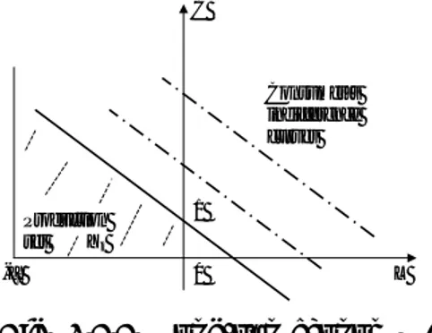
Case 1. Consider a 2 × 2 fictitious economy represented by the Edgeworth box of Figure 2.5.1. Since the “agents” of a fictitious economy exhibit linear preferences, their indifference curves are straight lines. Here, the indifference
curves of the “agents” coincide and the initial endowment w is Pareto optimal. However, the outcome E of the limit-price mechanism does not correspond to w and thus involves trades.
b
a E
Fig. 2.5.1
This property, which is specific to the proportional rule, will be responsible for several features of our dynamics:
1. The vector field will be discontinuous,20 so we may rely on
Filip-pov’s (1988) solutions.21
2. Even if the true economy crosses an infinitesimally Pareto optimal point (in which case the marginal economy looks like the one depicted in Figure 2.5.1), non trivial infinitesimal trades will occur.
3. This property of the proportional rule will lead to short-run un-deremployment, as shown in Example 1 of Section 3.
Infinitesimally Pareto optimal points turn out to be compatible with under-employment. In fact, Example 1 of Section 3 shows that it is possible for an economy to converge to full employment even though its starting point was al-ready infinitesimally Pareto optimal. With this in mind, feature 2. should rather be interpreted as a positive property. On the other hand, Examples 2 and 3 of Section 3 show that underemployment arises in our dynamics even when the pro-portional rule is not at work. Thus, the propro-portional rule is not solely responsible for involuntary unemployment; it is but one of the various causes of the failures of labor markets.
Case 2. Consider a fictitious linear economy such as that depicted in Figure 2.5.2, with no Walrasian equilibrium and for which the initial endowment ω is not Pareto optimal. In order to improve the situation of “agent” 1, one must take from “agent” 2 some good that has zero utility for him and then give it to “agent” 1. The limit-price mechanism selects the no-trade solution, so the final outcome is not Pareto optimal. As a consequence, solution paths of our dynamics can be trapped at points that are not Pareto-optimal (this was the qualification alluded to at the end of Section 1). However, the no-trade solution is Pareto
20This was already the case in the pure-exchange situation; see Giraud (2007). 21Filippov’s definition is recalled in the Appendix, Section 6.3.
optimal when computed in strict trades (as defined in Section 4.1). This will enable us to prove convergence of our solution paths to a weaker notion than mere Pareto optimality.
Fig. 2.5.2
2.6
The dynamics
Wrapping up everything, we define a marginal equilibrium ( ˙x(t), ˙y(t), ˙s(t), p(t)) of the economy Tx(t),y(t),s(t)E at time t as being the marginal outcome of its associated
order book O(t).
Recall that for (x, y, s) ∈ τ∗× RM
+ we use MO(x, y, s) to denote the subset of
marginal outcomes of the economy E in state (x, y, s). The sets M(x, y, s) and
P (x, y, s) will denote the corresponding marginal quantity outcomes and marginal
prices respectively:
M(x, y, s) :=
n
( ˙x1, ..., ˙xN, ˙y1, ..., ˙yM) ∈ R2(N +M ) | ∃p ∈ R2+ :
( ˙x1, ..., ˙xN, ˙y1, ..., ˙yM, p) ∈ MO(x, y, s)
o
,
P (x, y, s) :=
n
p ∈ S+2 | ∃( ˙x, ˙y) ∈ R2(N +M ) : ( ˙x, ˙y, p) ∈ MO(x, y, s) o
.
A trade and production path (x(·), y(·), p(·)), is a maximal Filippov solution22
of the differential inclusion ¡
˙x(t), ˙y(t)¢= M¡x(t), y(t)¢ and p(t) ∈ P (x(t), y(t)) a.e. t ≥ 0, (6) with x(0) = ω, and y(0) = y.
3
Examples of underemployment
Let us first propose various understandings of underemployment. We start by distinguishing three types of demand: (α) market demand for good c, denoted
MDc(p), which is the aggregate demand observed on the market (through the
ag-gregate limit orders) at every vector p; (β) maximal Walrasian demand, W Dc(p∗),
which is the maximal (in terms of volume) demand satisfied at some Walrasian equilibrium price p∗ (when it exists) of the fictitious linear economy induced by
some order book; and (γ) realized demand, RDc(p), which is the demand
sat-isfied at a marginal outcome induced by the proportional rule applied to some order book; here p is the marginal (short-term) price selected by the limit-price mechanism. Obviously, the three definitions do not coincide in general: As soon as some demand orders are not fully executed (or, equivalently, as soon as some player is rationed), MDc(p∗) will be larger than W Dc(p∗) (provided this latter
object is defined). As soon as the proportional rule comes into play, W Dc(p) will
itself be larger than RDc(p). Note that MDc(·) and RDc(p) are always defined,
whereas W Dc(p∗) may fail to exist.
Given these definitions, we can similarly define three different kinds of labor supplies (for each type of labor `): the market supply MS`(p), the maximal
Walrasian supply W S`(p), and the realized supply RS`(p). These lead to the
following definitions of underemployment:
(α) Walrasian underemployment, W U(p), is MS`(p∗) − W S`(p∗) ≥ 0
at some Walrasian equilibrium price p∗ of the linear fictitious economy
induced by some order book;
(β) realized underemployment, RU (p), is the difference W S`(p) −
RS`(p) ≥ 0 at the marginal price p (supposed to be also a Walrasian
equilibrium price);
(γ) market underemployment, MU (p), is the sum W U (p∗) + RU(p).
We shall see that all three types of underemployment emerge along trade and production paths of our dynamics. Clearly, RU(p) is entirely due to the proportional rule. Given a trade and production path, we define the natural rate of unemployment (NRU) as the limit of market underemployment MU(p(t)) as
t → ∞. Being the limit of the observed long term underemployment, the NRU
is affected by the history of observed underemployment. In this sense, hysteresis is accounted for.
3.1
Example 1: Realized “Classical” underemployment.
We assume that there is a single producer j facing a single consumer i. The production function of j is given by fj(yL) = −yL+ 1 with marginal productivity
inventory is sj(0) = yj = (0, 1). The consumer’s utility is linear and equal to
u(xL, xC) = xC + xL; also, (ωL, ωC) = 0, and aLi = 10.
L C -ai Production set Consumer’s indifference curves 0 Yj 1
Fig. 3.1.1. Long-run economy E
• At t = 0: At time t = 0, associated to T0,0,(0,1)E is the order book O, which
is generated by the limit-price orders of the limit-price mechanism, as described in Section 2. The underlying 2 × 2 Edgeworth box is represented in the next figure. The “endowment” of the (fictitious agent representing the limit-order sent by the) producer is e1 = (0, 1), and the “endowment” of the consumer is
e2 = (10, 0). The consumer (resp. producer) sends exactly one limit-price order
associated to the limit price equal to her (resp. its) marginal rate of substitution
MRS = 1 (resp. marginal productivity of labor MP L = 1).
10/11 1 C L L = 10C 10 L= -C + 1 0 1/11 1
Fig. 3.1.2. Order book t = 0
The line L = −C + 1 passing through the “endowment point” (0, 1) corre-sponds to the common indifference curve of the “agents” in the fictitious mar-ginal economy, and the proportionality rule selects the unique point at the in-tersection of the diagonal L = 10C and the common indifference line; (L, C) = (10/11, 1/11). The resulting price coincides with the unique (normalized) Walras equilibrium price of O: p∗ = (1/2, 1/2). The unique Walrasian allocation selected
by the limit-price mechanism among the continuum of Walrasian allocations is therefore (10/11, 10/11). In other words, the consumer has sold 10/11 of the ten units of labor put on the market. On the other hand, the producer has sold 10/11 unit of (unsold) consumption commodity put on the market. The realized demand of labor of producer j is 10/11 and his realized offer of goods is 10/11. Thus, at date t = 0, we have ˙yj(0) = (−10/11, 10/11), and ˙xi(0) = (−10/11, 10/11).
Market demand for C, MDC, is here equal to 10, maximal Walrasian demand
W DC = 1, and realized demand RDC = 10/11. Hence, both Walrasian and
1 pL / pC
L
1
Labor demand
curve Labor offer curve 10 10/11 Walrasian underemployment 1 1 pL / pC C Consumption offer curve Consumption demand curve 10
Fig. 3.1.3. Labor market t = 0 Fig. 3.1.4. Consumption market
t = 0
As shown in the figures above, there is excess labor supply and excess con-sumption demand in the marginal economy T0,0,(0,1)E. The economy starts at
t = 0 at a global and strict Pareto optimum; however, there are (infinitesimal)
trades induced by the proportional rule of the limit-price mechanism. In other words, (0, 1) is not a rest point of our dynamics.
• At t > 0: At time t = dt, the market labor offer is 10 − (10/11)dt, with p(dt) = p(0) = (1, 1). The indifference curve of the agents in the fictitious linear
economy associated to O at time dt is L = −C + 1, and the proportional rule
defines the curve L = 1
10−(10/11)dtC, from which the marginal outcome can be
computed. It is equal to C = 1 − 1
11−(10/11)dt. Hence, realized underemployment
increases and is equal to
³
1 − 1
11−(10/11)dt
´−1 .
Over time, the state of the economy evolves in a similar fashion along the boundary of the production set (or, equivalently, along the consumer’s indifference line). The consumer’s long-run utility remains constant. Let t = T denote the time at which the “agent” of the corresponding marginal economy offers exactly one unit of labor. For any t < T , there is labor supply rationing as well as short-run Classical realized underemployment. At t = T (see figure 3.1.5) there is no Walrasian underemployment any more but there is still realized underemployment by the proportional rule, according to which only half of the short-run labor supply is executed. 1 pL / pC L 1 Labor demand curve Labor offer curve 1/2
Fig. 3.1.5. Labor market t = T
moreover, ˙yj(T + dt) = ( 1/2dt − 1 2 − 1/2dt, 1 − 1/2dt 2 − 1/2dt).
We observe Walrasian excess consumption demand (in a broad sense). The econ-omy therefore displays contained inflation with realized underemployment.
1 pL / pC L 1 1-dt Labor demand curve Labor offer curve 1 pL / pC C 1-1/2dt Consumption offer curve Consumption demand curve 1 1/(1-dt)
Fig. 3.1.6. Labor market t = T + dt Fig. 3.1.7. Consumption market
t = T + dt
At date t > T (Figures 3.1.6 and 3.1.7), the economy moves slowly to (−10, 10), that is, towards full capacity utilization of labor, reached at some date t = ˆT ,
where trades cease. As a consequence, NRU = 0. In this simplistic example, the unique solution path of our dynamics is therefore a straight line connecting (0, 1) to (−10, 11). Every point on the trajectory is a global strict Pareto optimum (and also, of course, a strict infinitesimal Pareto point), both prices and the consumer’s long run utility remain constant. Hence, the producers’ myopic price expectations turn out to be rational. This shows there may exist Pareto optima that are not steady states of our dynamics, and short-run underemployment is compatible with global Pareto optimality.
Remark 3.1 If we assume in this example that there are no initial inventories (i.e., sj(0) = 0), then the starting point becomes a steady state of our dynamics.
It is a strict Pareto optimum and nevertheless NRU > 0.
3.2
Example 2: “Classical” underemployment
Take the same economy as before, except that now
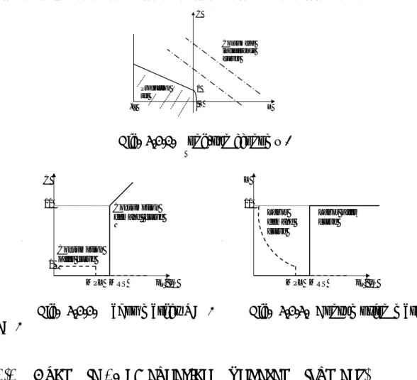
Yj = {(yL, yC) ∈ R−× R : yC ≤ 1 − 1 2yL} ∪ {(yL, yC) ∈ [0, ²) × R : yC ≤ −yL2 − 1 2yL+ 1} ∪ {(yL, ²) : yL≤ −²2− 1 2² + 1} and yj = (0, 1) (Figure 3.2.1).
At time t = 0, both the marginal productivity of labor at (0, 1) (1/2 =
MP L < MRSCL) and the amount of inventories sj(0) = 1 put up for sale are
too weak: There is short-run underemployment and no trade takes place for all relative prices pL/pC ∈ [MP L, MRS). There is a continuum [MP L, MRS]
of marginal (short-run) price vectors at t = 0. Thus, the example illustrates that our price dynamics may induce a continuum of final prices (although there is uniqueness along non degenerate trajectories, except at the limit; here, the problem clearly arises because the path is degenerate).
If pL/pC = MRS emerges then there is market underemployment, which can
be interpreted as Classical underemployment. The starting point is a steady state. Note that, because of the unsold inventories, it is not an infinitesimal Pareto optimum; NRU > 0. Here, evidently, a policy promoting the supply side should be implemented to increase the marginal productivity of labor MP L.
1 -ai L C Production set Consumer’s indifference curves
Fig. 3.2.1. Long-run economy E
Consumption offer curve MPL pL / pC C Consumption demand curve MRS 10 1 Labor demand curve MPL pL / pC L Labor offer curve MRS 10
Fig. 3.2.2. Labor market t = 0 Fig. 3.2.3. Consumption market
t = 0
3.3
Example 3: “Keynesian” underemployment.
Now, let fj(yL) = 2yL+ 1, sj(0) = 1, and u(xL, xC) = xC + xL with x(0) = 0.
Hence Yj = {(yL, yC) ∈ R−× R : yC ≤ −2yL+ 1}. In this case, the marginal
productivity of labor is too strong: MP L > MRSCL. Consequently, there is
underemployment at the marginal outcome of the marginal economy at time
L C Production set Consumer’s indifference curves -ai 1
Fig. 3.3.1. Long-run economy E
At time t = 0, the fictitious linear economy associated to the order book sent by the players in Tx(0),y(0),s(0)E admits a unique Walrasian equilibrium price
p∗
L/p∗C = 1; Figure 3.3.2 shows the Edgeworth box associated to this order book
at time t = 0: 1 C L 10 1/2 1 producer consumer
Fig. 3.3.2. Edgeworth box at t = 0
1 pL / pC C 1 Consumption offer curve Consumption demand curve 2 2 10 1 pL / pC L 1/2 Labor offer curve Labor demand curve 1 2 10
Fig. 3.3.3. Consumption market t = 0 Fig. 3.3.4. Labor market t = 0 At time t = 0, the limit-price mechanism selects the price (1, 1) together with ˙yj(0) = (−1, 2), βj(0) = (−1, 1), ˙xi(0) = (−1, 1), and sj(0) = dt ( ˙sj(0) = 1).
Note that the proportional rule does not apply (see Figures 3.3.3 and 3.3.4). At time t = 0 there is market underemployment but no realized underemployment. At t = dt, we have ˙yj(dt) = (−1 − dt, 2 + 2dt), ˙xi(dt) = (−1 − dt, 1 + dt),
There is market underemployment until some finite T ; at t = T , there is full market employment and NRU = 0. For t > T , firms are rationed on the labor market. Prices p(t) increase from pL/pC = MRS to pL/pC = MP L and then
stay equal to MP L. Let T∗ denote the first time t for which p(t) = MP L. The
trajectory of the dynamics is linear for t ≤ T and for all t ≥ T∗. For MRS <
pL/pC < MP L (i.e. T ≤ t ≤ T∗), the path is nonlinear. The economy converges
to a point in ∂τ with full employment, but it is neither a Pareto optimum nor an infinitesimal Pareto optimum because there remain unsold inventories. This example shows that full employment is compatible with Pareto suboptimality.
In our opinion, this example displays “Keynesian” underemployment (except at the limit) in the following sense. The effective consumption demand that is addressed to the firm on the consumption market is equal to 1 for t = 0 to t = T , whereas the consumption offer is at least 1 + dt for each t > 0. Hence there is a lack of effective demand, which prevents the firm from hiring more employees.
k
l
c
-10
10
Fig. 3.3.5. The path
One may wonder why the (Walras) equilibrium price (pL, pC) = (2, 1) is not
selected by our mechanism as a marginal outcome of the economy at time t < T . The reason, as already suggested in section 1, is that the output produced at time t − dt is too low for (pL, pC) = (2, 1) to emerge. Were the producer able to
put up for sale 20 units of consumption good rather than 1, then (pL, pC) = (2, 1)
would be the unique market-clearing price (see Figures 3.3.3 and 3.3.4).
4
Results
4.1
Preliminaries
In the next definition we consider an order book O.
Definition 4.1. In O viewed as a linear fictitious economy, a strict trade is a feasible trade ˙x ∈ τO such that, for all h, either ˙xh ≥ 0 or bh· ( ˙xh+ eh) > 0. Here
bh is the “utility vector” of “agent” h.
Extend functions ui : τ → R (i = 1, ..., N ) by ui(x, y) := ui(xi).
(1) An admissible curve is a smooth curve φ : [0, ε) → τ with φ(0) = (x, y) and d
dt(ui(φ(t))) ≥ 0 for all i, t ∈ [0, ε), with a strict inequality for at least one
individual i, at every t.
(2) A strict admissible curve at x is an admissible curve that passes through
x at some time t ∈ (0, ε) and such that φ0(t) is a strict trade in the order book
associated to Tx,y,sE.
(3) (x, y) ∈ τ belongs to θ (resp. Θ) if and only if there is no admissible curve that passes through (x, y) (resp. no strict admissible curve at (x, y)).
(4) For K ∈ {θ, Θ}, K∗ is the subset of points in K that are individually
rational with respect to long-run utilities.
Remark 4.1 Observe that, when (x, y) ∈ Θ, the short-term equilibrium price fails to be unique (even after normalization). This is one reason why we end up with an inclusion instead of an equality in (8). Another reason is that, at infinitesimal Pareto allocations, the short-run outcome may induce price vectors that do not sustain this very Pareto point as a price quasi-equilibrium.23
Infin-itesimal Pareto points (computed with strict trades) are also the unique points where indeterminacy of prices occurs.
Lemma 4.1. Under (C)-(i)-(ii) and (P), a point (x, y) of τ belongs to θ if and
only if there exist vectors p ∈ R2
+ and λ ∈ RN+ such that p, λ 6= 0 and:
(a) λibi ≤ p, ¡ p − λibi ¢ ·¡xi+ (ai, 0R) ¢ = 0 for all i ;
(b) p ∈ Nyj(∂Yj), the normal half-line to ∂Yj at yj, for all j.
Proof. This follows from first-order conditions. (See e.g. Mas-Colell (1985,
The-orem 4.3.1)), and take (−aL
i + R+) × R+ as the consumption set for household
i.)
¤ Assumption (C∗). Assumptions (C) (i) and (ii) are in force; in addition,
∇ui| ˆX∗
i(·) >> 0 for every i.
Assumption (D). For each j and each p ∈ S2
+, the map fp : Yj → R (which
sends yj ∈ Yj to p · yj) has exactly one critical point, and that critical point is a
non degenerate maximum.
This restriction is borrowed from Smale (1976), and captures the strict convex-ity of each production set Yj. It will enable us to deduce that every infinitesimal
Pareto optimum is, in fact, globally Pareto optimal, as shown in the next lemma. Lemma 4.2. (1) Under (C∗) and (I)24, and for fixed x ∈ τ∗, the following three
statements are equivalent:
23For a definition, see Example 2 (cf. Mas-Colell (1985, Def. 4.2.12)).
24This is an irreducibility assumption, the technical details of which are found in Giraud
(a) (x(t), y(t)) ∈ Θ∗;
(b) 0 ∈ Fϕ(x(t), y(t)) and sj(t) = 0 for all j;
(c) bi(t) · ˙xi = 0, for all i, ˙x ∈ Fϕ(x(t)).
(2) If also (C)(iii) and (D) hold, then θ coincides with the subset of strict (global)
Pareto optimal points in τ .
Proof. Part (1) follows Giraud (2007), while Part (2) follows from Smale (1976),
and Giraud (2007).
¤
4.2
Existence and convergence
Given a trade and production path γ := (x(·), y(·)), it follows that (x∗, y∗) ∈ τ∗
is a limit point if there exists a sequence (tn)n ∈ RN converging to +∞ such that
(x(tn), y(tn)) →n→∞ (x∗, y∗). We denote by Ω(γ) the set of limit points of γ.
A stationary point (x, y) of our dynamics is such that 0 ∈ F (x, y), where F is defined as in (8) (Filippov (1988, p. 124). A trajectory (x(·), y(·)) is said to be
degenerate if there exists some time T for which (x(t), y(t)) is independent of t
for all t ≥ T .
Assumption (S). There exists at least one household i such that ui is strictly
quasi-concave on Θ∗.
Proposition 4.1.
(i) Under (C), (P) and (I), there exists a trade and production path. Every
such path satisfies:
(ii) for every t ≥ 0, (x(t), y(t)) ∈ τ and xi(t) + (aLi , 0R+) > 0 for every i; (iii) the function t 7→ ui(xi(t)) is non-decreasing for every i;
(iv) every limit-point with no unsold inventories is in Θ∗.
(v) If, in addition, (B) and (S)hold, then every trade and production path
admits limit-points and every limit-point is in θ∗.
Proof. (i) Observe first that the graphs of M(·) and P (·) can be expressed by
means of a first-order formula over the field R of real numbers. Thus, according to Tarski-Seidenberg’s theorem,25M(·) and P (·) are semi-algebraic mappings and
hence they are Borel-measurable. As a result, the set-valued map obtained from (8) by replacing f with M(·) and P (·) respectively, is upper semi-continuous, non-empty, convex valued, and compact valued. Consequently, existence of local absolutely continuous solutions (x(·), y(·), p(·)) : [0, T ] → τ × SL+C−1
+ for some
T > 0 follows from standard existence results for differential inclusions (see e.g.
Aubin and Cellina (1984)).
In order to show that this solution is a trade and production path, it suffices to check that every local solution remains in a compact subset. Indeed, as already observed in Champsaur and Cornet (1990), the standard proof that compactness
of the domain implies maximality of the solution carries over from the single-valued case to the multi-single-valued case. But compactness of the domain follows from the feasibility of every marginal equilibrium in every marginal economy,
X i ˙xi(t) = X j ˙yj(t),
and the fact that for every t ≥ 0, one has (x(t), y(t)) ∈ τ∗ — which is compact
according to assumption (B).
(ii) That every trade and production path stays within τ has just been proved. That xi(t) + (aLi, 0R+) > 0 for every i and t is a consequence of the monotonicity of preferences, the individual rationality of each short-term outcome (Giraud (2007)) and the condition ωi+ (aLi, 0R+) > 0 for every i (Assumption (C)).
(iii) This, too, is a consequence of the individual rationality of trade and production paths; for a proof, see Giraud (2007).
(iv) The claim follows because (b) ⇒ (a) in Lemma 4.2.
(v) This follows from the standard argument; see Giraud (2007). ¤
5
Conclusion
To summarize, we briefly review some properties of the approach proposed here in comparison with the standard treatment of production in static general equi-librium theory.
1. Existence of a trajectory obtains in our setting in more general circum-stances than that of static competitive equilibria in Arrow-Debreu economies. In particular, we do not need the strong survival assumption that was shown by Kamiya (1988) to be a necessary condition for the existence of marginal cost pricing equilibria.
2. Whenever production sets exhibit increasing returns to scale, the behavior of a non-regulated firm can still be defined as short-run profit maximization, whereas static GET needs to rely on some regulated pricing behavior (such as marginal cost pricing, etc.). Even in this case, such a regulated firm may incur losses at a static competitive equilibrium, which makes sense only if it is publicly owned. There is room in our model for a theoretical debate about the need for publicly regulating firms with increasing returns. The reasoning runs as follows. Since no firm incurs losses along a solution trajectory, it makes sense to study the efficiency properties of a privately owned firm whose production set exhibits non convexities and to compare them with what could be obtained in a publicly regulated fashion.
3. When production is strongly convex (in the sense of Assumption (D) supra), steady states of our dynamics are always first-best optimal as soon as there are no unsold inventories. When production exhibits non convexities, steady states of