Differential rotation between lithosphere and mantle: a consequence of lateral mantle viscosity variations

HAL Id: hal-02046601

https://hal.archives-ouvertes.fr/hal-02046601

Submitted on 2 Feb 2021

HAL is a multi-disciplinary open access

archive for the deposit and dissemination of

sci-entific research documents, whether they are

pub-lished or not. The documents may come from

teaching and research institutions in France or

abroad, or from public or private research centers.

L’archive ouverte pluridisciplinaire HAL, est

destinée au dépôt et à la diffusion de documents

scientifiques de niveau recherche, publiés ou non,

émanant des établissements d’enseignement et de

recherche français ou étrangers, des laboratoires

publics ou privés.

Differential rotation between lithosphere and mantle: a

consequence of lateral mantle viscosity variations

Y. Ricard, C. Doglioni, R. Sabadini

To cite this version:

Y. Ricard, C. Doglioni, R. Sabadini. Differential rotation between lithosphere and mantle: a

conse-quence of lateral mantle viscosity variations. Journal of Geophysical Research, American Geophysical

Union, 1991, 96 (B5), pp.8407-8415. �10.1029/91JB00204�. �hal-02046601�

JOURNAL OF GEOPHYSICAL RESEARCH, VG ,. 96, NO. B$, PAGES 8407-8415, MAY 10, 1991

Differential Rotation Between Lithosphere and Mantle'

A Consequence

of Lateral Mantle Viscosity Variations

YANICK RICARD 1

Dipartimento di Fisica, Settore Geofisica, Universitd di Bologna, Italy

CARLO DOGLIONI

Dipartimento di Scienze Geologiche, Universitd di Ferrara, Italy

ROBERTO SABADINI 2

Dipartimento di Fisica, Settore Geofisica, Universitd di Bologna, Italy

The description of plate motions in the so-called hotspot reference frame introduces a global rotation of the lithosphere with respect to the mantle. This rotation, called toroidal field of degree 1, is roughly westward. It reaches an amplitude of about 2 cm/yr and has been consistently found in the different generation of plate tectonic models. Various authors have tried to relate

this observation to the deceleration of the Earth's rotation, to polar wander, or to tidal drag.

However, these different physical mechanisms cannot explain the requested amplitude. In this paper, we compare the values of this rotation vector using different relative plate motion models expressed in the hotspot reference frame. In a model Earth with lateral viscosity variations, a differential rotation is predicted. The observed net lithospheric rotation is consistent with the dynamics of a model Earth where the asthenospheric viscosity below the oceans is at least one order of magnitude lower than underneath the continents. This relative westward drift of the lithosphere may account for the significant structural differences between east or west dipping subduction zones.

THE DIFFERENTIAL ROTATION BETWEEN LITHOSPHERE AND MANTLE

The motions between plates are computed from three in- dependent data sets. The first consists in the spreading rates on ridges deduced from the Earth's magnetic inver-

sions recorded in the frozen mid-oceanic basalt. The sec- ond set includes the strikes of the transform faults which

are assumed to be parallel to the relative motions. Finally, the earthquakes slip motions help to constraint the motions particularly at shear or converging boundaries. From these data, only relative motions can be deduced. The choice of an origin in the angular velocity space specifies an absolute reference frame. Of course, the most natural frame would be the one in which the deep mantle has no rotation. Differ- ent criteria have been proposed to define practically such a

frame. Le Pichon [1968] implicitly suggests

that the Antarc-

tic plate remains fixed. Following

Burke and Wilson [1972],

it is the African plate that could be stationary with respect to the underlying mantle. The most widely accepted ref- erence frame is the one in which the hotspots remain fixed

[Wilson, 1965; Morgan, 1971]. These three hypotheses,

al-

though conceptually different, lead to the same conclusion: the lithosphere has a west trending average rota•ion.

Quantitatively, this lithospheric rotation f•œ c n be com-

puted

from the surface

plate velocity

V œ by the following

1Now

at Ddpartement

de Gdologie,

Ecole

Normale

Sup•-

rieure, Paris, France.

:•Also

at Istituto di Mineralogia,

Universit&

di Ferrara,

Ferrara, Italy.

Copyright 1991 by the American Geophysical Union.

Paper number 91JB00204.

0148-0227/91/91 JB-00204505.00

equation:

f•L= 3 /VLx,.

dS,

(1)

where ur is the unit radial vector and So is the Earth's sur- face. This net rotation can also be deduced from the expan- sion of surface velocities in vector spherical harmonics. The rotation is simply proportional to the toroidal coefficients of degree 1.

Minster et al. [1974] have computed the lithospheric rota-

tion of their AM1 model. It amounts

to 0.11ø/m.y. around

expressed in the hotspot reference frame. In that case, the

lithospheric

rotation reaches

0.26ø/m.y. (2.8 cm/yr) around

66øE and 54øS. We also used the HS2-NUVEL1 model

[DeMets et al., 1990; Gripp and Gordon, 1990]. Follow-

0.32ø/m.y. (3.6 cm/yr) around 64øE and 52øS.

The last two models (AM1-2 and HS2-NUVEL1) have

spheric rotations is thus only related to the difference in the relative velocity models. The selected hotspots were only located on, or very close to, the Pacific plate. On the contrary, the AM1 model was constructed using 20 hotspot tracks sited on eight different plates. However, for the slow moving plates, the actual azimuth of the hotspot chains can- not be precisely observed.

To be sure that our estimation of the net lithospheric rota-

tion is not strongly biased by the weight of the Pacific area

nor unrealistically influenced by the selection of imprecise traces, we perform another inversion. We only select traces

8408 RICARD ET AL.: DIFFERENTIAL ROTATION OF THE LITHOSPHERE

samphng different plates where the absolute velocity is a pri- ori known to be of order or larger than 1.5 cm/yr. The traces are all taken from the data that entered in the construction of the AM1 model. There are also consistent with the obser-

vations of Morgan [1972]. The inversion

is performed with

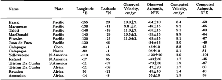
the 14 hotspots listed in Table 1. As Minster and Jordan

[19781,

we use both observed

velocities

(five data), and ob-

served azimuths (14 data). The first nine traces were used

for the determination of AM1-2 and HS2-NUVEL1; we add

five more to ensure a better geographical coverage. We chose

NUVEL-1 for relative plate motion model and we only read-

just the global rotation to match our selected data. Our

inversion indicates that the lithosphere has a net rotation of

0.15ø/m.y. (1.7 cm/yr) around a pole situated at 84øE and

and azimuth of the chosen hotspot traces according to our

model. All the computed values but two (Marquesas

and

Galapagos

on the Nazca plate) lie within the prescribed

un-

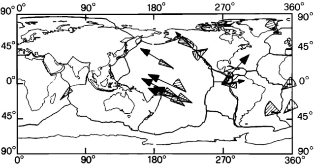
certainties. Figure 1 shows the localization of our hotspots

on top of a map depicting the tectonic plates taken into ac-

count by NUVEL-1. The hotspot velocities deduced from

our inversion are also plotted with the observed directions

and a priori uncertainties.

Gar[unkel et al. [1986] have suggested

that the discrep-

ancy between the hotspot reference frame and the no-net

rotation frame is a bias due to an overestimate of the mi- gration rates for the Pacific volcanoes. However, the AM1 model was constructed by only fitting the trends of hotspots without taking into account their absolute velocities. Simi- larly, we also performed an inversion only using the azimuths of our selected hotspots. A global rotation was still found

with a rotation pole consistantly located in the southern

part of the Indian Ocean but with the smaller amplitude of 1.0 cm/yr.

Although different, the estimations of the net lithospheric rotation agree with a roughly westward rotation with a pole

located in the southern part of the Indian Ocean and an observed velocity of a few centimeters per year. The Pacific hotspots seem to have a relative velocity with respect to the other hotspots which explains the discrepancy between the models. However, it should be clear that this exercise cannot be a test of the hypothesis of hotspots fixity. The

relative plate motion models are only valid for the present time and the very last million years, whereas the hotspots fixity applied for a much longer time.

Figure 2 shows

the pole, labelled a, of the net lithospheric

rotation deduced from our inversion. This rotation is clearly related to the total motion of the Pacific plate. The three

poles labelled b, c, and d corresponding to models AM1, AM1-2, and HS2-NUVEL1 are also plotted with a circle whose size is proportional to the amphtude of the motion. The solid circle will correspond to the result of a model and will be discussed later. Due to map distortion at high latitudes, the different poles look rather distant, but their

angular

distance

is at most 300

.

On the basis of geological observations, various authors

have also advocated

for this differential rotation [Nelson

and

Temple,

1972; Uyeda and Kanamori, 1979; Do91ioni

1990].

tion of the mantle. The main differences are summarized in

Figure 3. Of course, these two types of thrust belts should

West dipping subductions have a steep inclination of the

slab and are associated

to back arc basins

(e.g., West Pacific,

Barbados, Sandwich, Apennines, Carpathians). Thrust

belts related to this kind of subduction (contrasting the

mantle flow) show low structural and morphologic

reliefs,

obstacles to the westward flow of the lithosphere.

East dipping slabs have a shallow dip and are not as-

sociated to back arc extensional basins (e.g., American

Cordillera, Western Alps, Dinarides, Zagros). Thrust belts

related

to this kind of subduction

(following

the mantle

flow)

TABLE 1. Hotspot data used to compute the Absolute Motion Model

Observed Observed Computed Computed

Name Plate Longitude Latitude Velocity, Azimuth, Velocity, Azimuth,

øE

ON

cm/yr

NøE

cm/yr

NøE

Hawai Pacific -155 20 10.04-2. -644-10 8.4 -59

Marquesas Pacific -138 -11 9.8 4-2. -454-15 9.2 -65

Tahiti Pacific -148 -18 11.04-2. -654-15 9.1 -63 MacDonald Pacific -140 -29 10.54-2. -554-15 8.9 -64 Pitcairn Pacific -130 -25 11.04-2. -65 4-15 9.1 -67 Juan de Fuca Pacific -130 46 -544-15 5.0 -46

G alapagos Coco -92 - 1 45 4-10 8.8 43

G alapagos Nazca -92 - 1 95 4-10 5.1 81

Yellowstone N.America - 110 45 - 120 4- 20 2.0 - 101 Iceland N.A merica - 17 65 -43 4- 30 1.7 -45 Tristan Da Cunha S.America -11 -37 -734-30 1.9 -87 Tristan Da Cunha Africa -11 -38 474-20 1.7 60

Reunion Africa 56 -21 454-10 1.4 40

Ascension Africa - 14 -8 55 4-10 1.5 58

The observed azimuths and rates with their uncertainties are shown in comparison with the predictions deduced from our

RICARD ET AL.: DIFFERENTIAL ROTATION OF THE LITHOSPHERE 8409

0

90

ø

90

ø

180

ø

270

ø

360

ø

90 ø

45ø

•

45ø

0

/'

00

45 ø

•

45 ø

90 ø

I

I

I

90 ø

0 ø

90 ø

180 ø

270 ø

360 ø

Fig. 1. Selected hotspots used in our computation of the global lithospheric rotation. The azimuth of the observed trends with

their estimated uncertainties are also plotted. The arrows correspond to the velocities deduced from the NUVEL-1 model. Their amplitudes are listed in Table 1.

show

huge exposures

of basement

rocks, high structurM and

morphologic

reliefs in contrast to limited and usuMly shal-

The two kinds of subductions provide different metamor-

phic paths for the relative thrust belts. Only in the east

dipping thrust belt, coesite-pyrope

bearing assemblages

and

eclogites

have been found [Chopin,

1984; Wang et al., 1989],

indicating that confining

pressures

between 20 and 30 kbar

the overthrusting lithosphere can account for this observa-

tion (Figure 3). In the east dipping subductions

the basal

als. On the contrary, the metamorphosed rocks sink into the

mantle under West-dipping subductions.

Oceanic ridges, continental rift zones, and subduction trenches are generally perpendicular to the differential veloc-

ity field depicted in Figure 2. The main deviations from this rule are only found in the North Atlantic ridge, the western portion of the southwest Indian ridge, and the Philippine subduction arc. On the contrary, the major shear zones appear to be parallel to the observed differential velocity.

90o0

ø

,

45

ø

90 ø

,

••/

/

/

]

0 ø

90 ø

180 ø

270 ø

90 ø

180 ø

270 ø

360 ø

90 ø

45 ø

0 ø

45 ø

90 ø

360 ø

Fig. 2. Net rotation of the lithosphere with respect to the deep mantle. The rotation pole has been deduced from the observations

of 14 hotspot traces using the relative motion model NUVEL-1 (a). The maximum velocity reaches 1.7 cm/yr. We also show the lithospheric rotation poles of the different models AM1 (b), AM1-2 (c), and HS2-NUVEL1 (d) with a circle with size proportional to

8410 RICARD ET AL.: DIFFERENTIAL ROTATION OF THE LITHOSPHERE

w

•:'-:'•..:!;i•ii

to the

lithosphere

Fig. 3. Comparative

sketch

between

the west

and

east

dipping

subductions

connected

to the relative

eastward

mantle

motion.

In

the

west

dipping

subduction

case,

the

slab

acts

as an obstacle

to the

eastward

mantle

flow

and

back

arc

extension

develops

due

to

the

lithospheric

loss.

This

will

produce

an eastward

migration

of the

tectonic

setting

and

a pronounced

foredeep.

The

base

plate

detachment

is in this

case

folded

and

subducted.

East

dipping

subduction

has

a shallow

dip.

The

basal

detachment

of

the

eastern

plate

is reaching

the surface;

this

provides

a mechanism

to bring

deep

crustal

levels

of the thrusting

plate

at the surface.

The subduction

hinge

is in this

case

westward

retreating.

The

morphological

relief

of the

thrust

belt

related

to the

east

dipping

subduction

is much

more developed with respect to the east dipping case.

FAILURE OF RADIALLY STRATIFIED EARTH MODELS

The observation

of this differential

velocity

leads

to an old

and puzzhng

problem.

Mechanically,

in a radially

stratified

Earth, the canonical reference

frame should be the one in

which

the lithosphere

has

no-net

rotation

[Lliboutry,

1974].

In effect, the Navier-Stokes

equations

applied

to a mantle

where the viscosity

variations

are only radial indicate that

the toroidal

velocity

field of degree

1 (global

rotation)

is

uniform

through

the mantle

[Ha9er

and O'Connell,

1981].

This means

that the toroidal

stress

field of degree

1 is zero

as

a consequence

of free slip boundary

conditions

which

prevail

at the Earth surface.

The possibility

of inducing

a westward

drift by tidal drag

has

been

suggested

[Bostrom,

1971;

Knopoffand

Leeds,

1972;

Moore,

1973].

However,

Jordan

[1974]

has

clearly

shown

that

tidal drag is far from being significant

and that this mech-

anism should

be abandoned.

Furthermore,

we saw that the

observed

global

rotation

has a pole

differing

significantly

to

the Earth's pole of rotation. A change

in the Earth's rota-

tion pole (true polar wander)

would

induce

a poloidal

field

related

to the readjustment

of the equatorial

bulge

[Sabadini

et al., 1990]. It is also responsible

for a global

rotation

of

the geography

with respect

to the inertial

reference

frame,

but it does

not produce

any significant

differential

rotation

between the lithosphere

and the mantle.

Any other possible

explanation

of lithospheric

rotation

invoking

the application

of a net torque

will fail because

it

would change,

or even reverse,

the Earth's rotation in a few

months

for any realistic

mantle viscosities.

A simple

nu-

merical

estimation

can illustrate

this point. To produce

a

differential

motion

of 1.7 cm/yr over

an asthenospheric

chan-

nel with a thickness

of 100 km and a viscosity

of 1019

Pa s,

a equatorial

stress

of 5. x 104 Pa s must

be applied.

This

low level

stress

will produce

on the whole

lithosphere,

a net

torque

of 1. x 1025

Pa s. Such

a torque

will change

the

rotation period of the Earth whose moment of inertia is

8 x 1037

kg m -2 by the totally

unrealistic

value

of 2.5 min

every day! Therefore,

to explain the observation,

we must

The motions

of the plates are induced

by the balance

of

driving

and resistive

torques.

The driving

torque

is related

to the lateral density variations in the mantle. It is induced

by the negative

buoyancy

of the downgoing

slabs

or to the

positive

buoyancy

under the ridges.

This torque

can be re-

lated to the mantle

circulation

[Ricard

and Vigny,

1989],

or alternatively

to the well-known

boundary

forces

such

as

slab

pull and ridge

push

[Solomon

and Sleep,

1974;

Forsyth

and Uyeda,

1975]. The resistive

torque

is the consequence

of the drag imposed

by the moving

lithosphere

to the vis-

cous

asthenosphere.

It is generally

assumed

that the drag

•.L obeys

a simple

viscous

law,

so

that

the

drag

force

is lin-

early

proportional

to the lithospheric

velocity

V L. The drag

coefficient

K may be regionally

variable.

The relationship

between these quantities reads

(2)

This equation

implies

two assumptions.

The first is rather

obvious

and assumes

that the velocity

at the surface

of the

mantle is equal to zero. This hypothesis

could be valid if

there

is a strong

decoupling

between

the lithosphere

and

the

underlying

mantle. The second

is more delicate

but cannot

be physically

sustained.

It supposes

that even

a net torque

applied

to the mantle

does

not induce

a global

rotation

of

the Earth. This

implies

that the mantle

is not only

rigid

but also

is maintained

fixed

in space.

We must

thus

change

RICAR, D ET AL.: DIFFERENTIAL ROTATION OF THE LITHOSPHERE 8411

r =

_

where

V M is the mantle velocity

beneath

the lithosphere.

If we make again the hypothesis that the mantle is rigid,

we must

impose

that the net average

of r œ is zero

and that

V M is a rigid rotation.

These

conditions

were

not realized

by equation (2).

By inspection

of equation (3), we see that if the coupling

where Pi are simple matrices formally identical to inertial

matrices for a body of equivalent surface density Ki =

+

z

h = / Ki a:y

zy zz )

--(x • q- z 2)

yz

ds.

yz

-(a: +

(s)

coefficient

K is

constant,

when

the

net

average

of r L is equal

Equation

(7)

is

clearly

independent

from

the

reference

frame

to zero,

the

net

differential

rotation,

which

is the

average

of as

the

addition

of a given

rotation

vector

Q to all the

plate

V œ

- V M is also

equal

to zero.

Only

the

coupling

between

rotation

vectors

Qi, induces

the

same

amount

of rotation

Q to the mantle. Therefore we can deduce from equation the lateral variations of K and the surface velocity can lead

to a zero

average

of r œ and

a nonzero

average

of V œ

- V M.

We can also see that even with variations in the coupling

between lithosphere and asthenosphere, a pure rigid rotation at the surface induces a pure rotation of the whole planet

without associated stresses.

Quantitatively, we can estimate the value of K by consid- ering that between the surface and the depth H, the Earth

has a variable viscosity

r/(r, 8, c•). In a thin shell approxi-

1

V

L - V

M = H(•)r

L,

(4)

where

(l/r/) is the vertical

average

other the depth H of l/r/

and is a function of latitude and longitude. In this equation, H is the thickness of an outer shell which contains all the

(7) the net rotation of the lithosphere-Q0 when we chose

for Qi the rotation poles of the plates in a no-net rotation

frame.

We could have tried to find the function K which should

be used in equation (6) in order to exactly fit the ob-

served rotation pole. Unfortunately, the inversion of the

two-dimensional continuous function K using only the ob-

served three components of the differential velocity is highly

nonunique. However, we saw that the rotation is clearly re- lated to the Pacific plate motion, i.e., to the main oceanic plate. From seismic tomography, it also appears that con- tinents and oceans are strongly differentiated in the top of the upper mantle. Therefore, to test our approach, we use a very simple model for the coupling function K. We assume that the coupling coefficient K is equal to 1 under oceanic

areas and K½ under continental ones.

Figure 4 depicts the misfit deduced

from equation (7),

lateral

viscosity

variations.

This

thickness

is supposed

to v/(f•at _ •bs)2 expressed

in centimeter

per

year

as

a func-

be smaller

than the characteristic

length of the plates. By tion of Ke. When Kc = 1 the differential

velocity

is equal

comparing

equations

(3) and (4) we see

that we can write to 0 and the misfit is equal to the net rotation

that we de-

I -1

K = (H(•)) .

(5)

DIFFERENTIAL VELOCITY FOR A RIGID MANTLE Our aim is to verify that using a realistic coupling func-

tion, equation (3) can explain the observed

lithospheric

ro-

tation. Of course, this equation does not describe all the kinematics of the plates. On the real Earth, the driving forces, which are not considered here, induce a torque which cancels the one produced by the resistant stresses of equa-

tion (3).

A simple calculation can be done in a model where the

rigid plates are moving on top of a rigid mantle. We have

seen that the mantle velocity is described by a pure rotation ft0 whereas the surface plate is described by i rotation vec- tors Qi, where i is the number of plates. The requirement

that the net torque must vanish leads, using equation (3),

to

x x

d,

= f c(n0

x x d,,

i

where t•(i, 0•b) is 0 or 1 depending

whether 0•b points to the

i th plate

or not. After expressing

the double

vectorial

prod-

uct, equation (6) reads

duced from NUVEL-1, 1.7 cm/yr. The misfit function shows

der continents than under oceans. In this case the observed

misfit is around 0.3 cm/yr, a value which is smaller than the

differences between the estimations of the observed global rotations deduced from AM1, AM1-2, and HS2-NUVEL1.

1 lO 2 i i i i i i i i • i i 1.5 0.5

01

Fig. 4. Misfit between the observed and computed net rotation of the lithosphere in centimeters per year as a function or the ratio between the continental and oceanic coupling coefficients. The coupling ratio is plotted on a logarithmic scale.

8412 RICARD ET AL.: DIFFERENTIAL ROTATION OF THE LITHOSPHERE

At the minimum the computed rotation is of 1.7 cm/yr

around a pole located at 93øE and 47øS. The corresponding

pole is plotted on Figure 2 (solid circle). Our model indi-

cates a preferred value of around 7 for the viscosity increase

between oceanic and continental regions. This number rep- resents the ratio of the vertically averaged inverse viscosity

of the two domains (equation (5)). At a given depth, the

The good fit realized by our simple model suggests that the real lateral viscosity variations are indeed, closely re- lated to the ocean-continent distribution. Of course, the remaining misfit must not be interpreted as associated to a

nonzero net torque applied to the mantle. It rather indicates

that the coupling function is not strictly proportional to the

ocean fiifi'Ction.

DIFFERENTIAL VELOCITY FOP, A VISCOUS MANTLE

In 'Order

to solve the equation

(3) for a more realistic

viscous mantle, we use the same mathematical formulation

as described

by Ricard et al. [1988]. This formulation as-

etry comprises one central sphere with radial mechanical properties, and an outer shell of thickness H in which the

viscosity also varies with latitude 0 and longitude •b. In this shell the lithospheric viscosity is */0 between the surface and

the depth œ(0, •b), then */1 in the asthenospheric

channel

ex-

tending from L(0,•b) to H. The radially averaged

inverse

viscosity

which enters

equation (4) reads

Z

=

-

(s)

In the inner sphere,

the dynamics

is suitaMy solved

by

the expansion

of the different quantities, such as velocities

and stresses,

on the basis

of generalized

spherical

harmonics

[Phinney

and Burridge,

1973]. Simple

relationships

between

the spectral

components

of r L and

V M can

be found

[Hager

and O'Connell,

1981; Ricard

et al., 1984, 1988]. These

rela-

tionships can be summarized as follows:

=

+

+

where the superscript

plus means

that this equation

stands

for the components

on the basis

of generalized

spherical

har-

monics. This equation indicates that when a horizontal ve-

locity

of poloidal

and toroidal

components

(vM) + is im-

posed at the surface

of a viscous

sphere

of radius R, the

associated

stress

field is obtained

by applying

the operator

F, which

multiplies

the poloidal

and toroidal

velocity

com-

ponents

of degree

I by k•/ and k}/. The variations

of the

averaged

horizontal

velocity

in the outer

layer (V} drive a

vertical flow at the converging

and diverging

zones,

which

induces

another

poloidal

stress

field described

by the coef-

ficient

k•/. This ensures

the mass

conservation

of the litho-

sphere

through

the zone

of subduction

and ridges.

In the outer layer, the flow is described

by the equation

(4). Other relationships

must be introduced

to define the

average

horizontal

velocity (V}. It reads

(v) = cv + (, - c)v

(11)

where

I L(L

-- H) */0

-- */1

(12)

C = • + H2 2,/o*/1(1/*/)

'

This equation

expresses

the horizontal

average

velocity

of a

Couette

tiow embedded

between

two boundaries

of velocity

V œ and V M.

The mathematical problem requires the solution of a set of

locM equations

(equations

(3) and (11)) and spectrM

equa-

tions (10). The two local equations

can be written in the

spectral domain'

(vL) + -- (vM) + = M 1

(TL)

4',

(13)

((V))

+ = M2(vL)

+ + (Id- M2)(vM)

+.

(14)

The two matrices M1 and M2 are computed

from the ex-

pansion

of ((1/*/) and C in spherical

harmonics.

They read

12ra21ama(1/*/)12m

• ,

(15)

M• (l• ra•, lsms)= •.

and

-12rn•larnaCl•rn (16)

M•li mi, lsms)=

••

•.

The coefficients - l:•rn:•lsrna

Ullml

are computed

using Wigner-3j

symbols

[Edmonds,

1960]

ol•m2larna

Ixra• -- (--1)

/x+rnx

•/(2/1

-[-

1)(2/2

4•'

-{-

1)(2/3

-{-

1)

(111213)(111213).

(17)

x --1 0 1

--mlm2m3

The -12rn21arna

coefficients

vanish

unless

m

2 = m

1 + m3,

[rn2]

_< 12, and [11

--131 _< 12 _<

11 + 13.

Using

equations

(10), (13), and (14), the problem

can be

solved;

when

V L is the plate

velocity

in a no-net

rotation

frame,

the toroidal

coefficients

of degree

1 of V M are

directly

proportional to the lithospheric rotation.

To avoid edge effects

in the description

of the inverse

vis-

cosity variations

in spherical

harmonics,

we have chosen

to

take the smooth function L(O, c•) whose

normalized

laterM

variations are depicted on Figure 5. This function is a fil-

tered version

of the ocean function and only contains

har-

monics

of degrees

smaller

or equal to 10. The grey areas

over continents

correspond

to a thick lithosphere,

whereas

the oceans

are underlaid by a thinner lithosphere.

'We chose

the amphtude

and average

value of the function L in order to

have a lithosphere

with a thickness

going

from 0 to H = 100

km. From equation

(9), the lateral variations

of the inverse

viscosity

are going

exactly

from the lowest

vMue

1/*/0 to the

highest value

In our formulation,

only the average

inverse

of viscosity

enters. The lithospheric thickness function that we have

used

is only an easy way to scale

our viscosity

variations;

of course, the real lithosphere cannot reach a zero thick- ness. Other heuristic models, such as a model with uniform

viscosity

underlain by an asthenosphere

with lateral viscos-

ity variations,

could

have

lead to the same

inverse

viscosity

function.

Beneath

the outer shell with its lateral viscosity

varia-

tions,

we consider

a mantle

made

up of two layers,

an upper

part with viscosity

*/u and a lower part with viscosity

RICARD ET AL.: DIFFERENTIAL ROTATION OF THE LITHOSPHERE 8413

90

ø

0 ø

90

ø

_...

180

ø

270

ø

360

_{90 ø}

ø

45 ø

...

45 ø

0 ø

0 ø

45

ø

0 ø

90 ø

180 ø

270 ø

360 ø

Fig. 5. Lateral variations of the average inverse viscosity in our outer shell. The grey continents correspond to a high viscosity, whereas the nonshaded oceans are underlaid by a lower viscosity. This normalized function is a filtered version of the ocean-continent distribution and only contains spherical harmonics of degrees smaller than 10. The local maxima in the oceans are due to Gibbs

effects

related

to the spectral

truncation.

The inverse

averaged

viscosity

is exactly

1/•/0 at its minimum

and 1/•/1 at its maximum.

ary. We ran the computation taking into account all the cou- pling coefficients up to a degree lmax going from lmax -- 10

to lmax -- 15. We verified that for lmax -- 15 an asymptotic

value was attained; the coupling of lateral viscosity varia- tions of degrees larger than 15 with velocity described by vector harmonics of degree larger than 15 will not signifi- cantly change our estimation of the lithospheric differential

velocity.

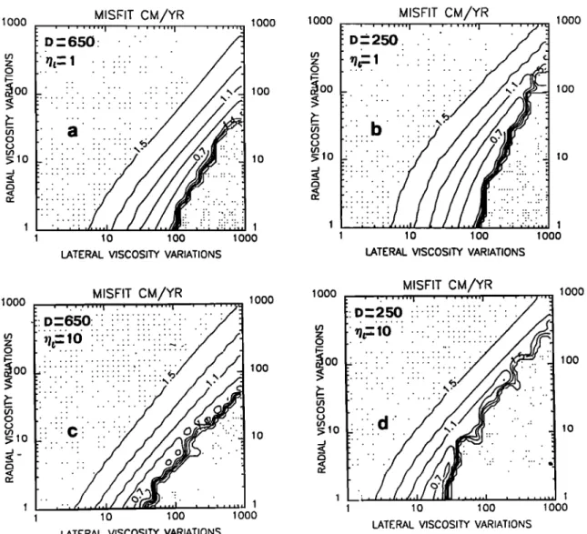
Figure 6 depicts by means of isolines the misfit between the observed and modelled differential rotation as a function of the ratios •0/•1 and •o/•u for different values of D and •11/•1o. Figures 6a and 6b are for •/1 = •/0; in Figures 6c and

6d, the viscosity in the lower part of the mantle has been

increased by a factor 10. In Figures 6a and 6c, the radiM

viscosity transition within the mantle is at the upper-lower

mantle boundary (D = 650 km); in Figures 6b and 6d the

viscosity

increase

lies below a thin low-viscosity

channel

(D

= 250 km).

In all graphs, the right lower part with the darkest shading represents a zone where the misfit is larger than 1.7 cm/yr and therefore larger than the signal itself. The smaller mis- fits are attained in the zone without shading. The best solu-

tions can explain more than 70% of the observation

(a misfit

of 0.5 cm/yr). This satisfactory

fit advocates

for a strong

correlation between the lateral viscosity variations of the real

Earth and the ocean-continent distribution. The lateral vis- cosity variations required are Mways larger than what has been found in the simpler model with a rigid mantle. How-

ever, if a viscosity contrast by a factor of 70 is required for a

uniform mantle (Figures

6a and 6b), an increase

of the lower

mantle viscosity

(Figure 6c) reduces

this contrast

to a factor

around 20 if we impose a viscosity increase just below an as-

thenospheric

channel

(Figure 6d). For a given upper mantle

a decrease in the necessary lateral viscosity variations' our

model tends to the asymptotic

limit we found for a rigid

mantle. For a given lower mantle viscosity, a decrease in

the upper mantle viscosity leads to an increase of the lateral viscosity variations: an inviscid asthenosphere would lead to a zero differential velocity.

CONCLUSIONS

The existence of a global westward rotation of the litho-

sphere

with respect

to the hotspots

is strongly

suggested

hotspot traces and of the absolute velocities chosen for the Pacific volcanoes. This rotation is a real one and is not an

artifact of the choice

of the reference

frame in which plate

motions

are defined. As a consequence,

an anchoring

ef-

fect of the subducted slabs in the mantle which is eastward

migrating is expected. This mechanism

could explain the

observed

larger dips of the west dipping subductions

which

contrast the mantle flow and the opening of the back arc

basins.

This net rotation is forbidden by the models where the Earth's properties are radially stratified. We show that a net rotation naturally appears in the models where lateral vis- cosity variations are allowed, the amplitude of this toroidal field being directly related to the amount of lateral varia-

tions. A similar conclusion

has been drawn by O'Connell et

al. [1991]. The observed

rotation with a pole in the southern

part of the Indian Ocean

and an amplitude

of 1.7 cm/yr can

ceanic

and subcontinental

mantle. Such a viscosity

contrast

agrees

well with seismic

tomography

of the upper mantle,

oceanic

regions. If these seismic

velocity anomalies

are ther-

mal or compositionM

in origin, we must expect lateral vis-

cosity variations

of 1 or 2 orders of magnitude. Further-

more, these lateral variations are also consistent with heat

flow data based

on the interpretation

of seismic

tomography

in terms of thermal and compositional

anomalies

[Yah et

8414 RICARD ET AL.: DIFFERENTIAL ROTATION OF THE LITHOSPHERE

lOOO

MISFIT

CM/YR

looo lO00

•

MISFIT

CM/YR

looo

• oo

1

oo

1 1 1

I

1o

1oo 1ooo

•

;AO•IATiONS

1000

MISFIT

CM/YR •oo0 lOOO MISFIT

CM/YR lOOO

1000 . .,..,.,.,,,•,•...,..,

,.,.'.v't..' .'.'.'"'

lO

•1o

lO

•TERAL

VISCOSITY

VARIATIONS

LATERAL

VISCOSITY

VARIATIONS

Fig.

6. Misfits

depicted

by

mea•

of

isolin•,

between

the

observed

and

computed

net

rotation

of

the

lithosphere

in centimeters

per

ye•. The

hori•ntg

a•s depicts

the

ratio

between

subcontJnent•

•d suboce•ic

viscosity

•0/•1. The

vertic•

axis

depicts

the

ratio

between

su•continent•

viscosity

•d the

viscosity

of the

top

p•t of the

upper

mantle

•0/•. Below

the

outer

shell,

the

mantle

viscosity

v•es

r•iily •d presents

a viscosity

imp at the

depth

D. This

depth

is

650

km

for

Fi• 6a

and

6c,

•d 2S0

km

for

Fi• 6• and

6d.

The

viscosity

o[

the

lower

p•t o[

the

mantle

is

1 in Fibres

6a

and

6b,

and

10

in Fi• 6c

and

6d.

al., 1989]. A substantial

decrease

of the upper

mantle

vis-

cosity

beneath

the oceanic

lithosphere

is also strongly

sup-

ported by the analyses

of the Holocene

sea level changes

in

oceanic island sites located in the far field with respect to

the Pleistocenic

Arctic and Antarctic ice sheets

[Nakada and

Larnbeck,

1989].

A trade-off exists between lateral and radial viscosity vari- ations. An increase in the lower mantle viscosity confines

the return flow more efficiently in the upper mantle and de-

creases

the amplitudes

of the requested

lateral viscosity

vari-

ations. Our calculations are consistent with lateral viscosity

variations

ranging

from one to two orders

of magnitude

be-

tween

continental

and oceanic

regions,

for any realistic

radial

It should

be emphasized

that in the present

modeling,

we

depth, assuming

that below this depth the lateral viscos-

ity variations

are of lesser

amplitudes.

This implies

that

we do not have any differential

rotation within the under-

lying mantle. The lithospheric

rotation

that we computed

is therefore a net rotation of the lithosphere with respect to

the whole mantle, independently

from the location

of the

hotspots sources.

Acknowledgments.

We are grateful

to G. V. Dal Piaz for useful

discussions.

One of us (Y. Ricard)

was a fellow

of ESA (Euro-

pean

Space

Agency)

at the University

of Bologna

(Italy). This

work has been partly supported by the INSU-DBT (Dynamique

et Bilan

de la Terre)

program

(contribution

270), and by the ASI

REFERENCES

Bostrom, R. C., Westward displacement of the lithosphere, Na- ture, •$J, 536-538, 1971.

Burke, K., and J. T. Wilson, Is the African plate stationary?,

Nature, •$9, 387-390, 1972.

Chopin, C., Coesite and pure Pyrope in high grade blueschists

of the Western Alps: A first record and some consequences,

C'ontrib. Mineral. Petrol., 86, 107-118, 1984.

DeMets, C., R. G. Gordon, D. F. Argus, and S. Stein, Current

plate motions, Geoph•s. J. lnt., 101,425-478, 1990.

Doglioni, C., The global tectonic pattern, J. Geod•n., 1•, 21-38,

1990.

Edmonds, A. R., Angular Momentum in Quant•tm Mechanics,

I•.ICAP•D ET AL.: DIFFEP•ENTIAL ROTATION OF THE LITHOSPHEP•E 8415

Forsyth, D., and S. Uyeda, On the relative importance of driving Phinney, R. A., and R. Burridge, Representation of the elastic-

forces

of plate motion, Geophys.

J. R. Astron. Soc., 43, 163.

gravitational

excitation

of the spherical

Earth model

by gener-

Garfunkel Z., C. A. Anderson, and G. Schubert, Mantle circula- 451-487, 1973.

tion and the lateral migration of subducted slabs, J. Geophys. Ricard, Y., and C. Vigny, Mantle dynaxnics with induced plate

.Res., 91, 7205-7223, 1986. tectonics, J. Geophys. .Res., 94, 17,543-17,559, 1989.

Gripp, A. E., and R. G. Gordon,

Current

plate velocities

relative Ricard, Y., L. Fleitout, and C. Froidevaux,

geoid heights

and

to the hotspots

incorporating

the Nuvel-1

global

plate motion lithospheric

stresses

for a dynaxnical

Earth, Ann. Geophys.,

2,

model, Geophys..Res. Lett., 17, 1109-1112, 1990. 267-286, 1984.

Hager, B. H., and R. J. O'Connell,

A simple global model of Ricard, Y., C. Froidevaux,

and L. Fleitout, Global plate motion

plate dyna•-nics

and mantle

convection,

J. Geophys.

Res., 86,

and the geoid,

a physical

model, Geophys.

J., 93, 477-484,

4843-4867, 1981. 1988.

Jordan, T. H., Some comments on tidal drag as a mechanism for Sabadini, R., C. Doglioni, and D. A. Yuen, Eustatic sea level

driving plate motions, J. Geophys..Res, 79, 2141-2142, 1974. Knopoff, L., and A. Leeds, Lithospheric momenta and the decel-

eration of the Earth, Nature, 237, 93-95, 1972.

Le Pichon, X., Sea floor spreading and continental drift., J. Geo- phys..Res., 73, 3661-3697, 1968.

Lliboutry, L., Plate movement relative to rigid lower mantle, Na-

ture, 250, 298-300, 1974.

Minster, J. B., and T. H. Jordan, Present-day plate motion, J. Geophys. .Res., 83, 5331-5354, 1978.

Minster, J. B., T. H. Jordan, P. Molnar and E. Haines, Numeri-

cal modelling of instantaneous plate tectonics, Geophys. J. R.

Astron. Soc., 36, 541-576, 1974.

fluctuations induced by polar wander, Nature, 345, 708-710,

1990.

Solomon, S.C., and N.H. Sleep, Some simple physical models for absolute plate motions, J. Geophys. Res., 79, 2557-2567, 1974. Uyeda, S., and H. Kanaxnori, Back arc opening and the mode of

subduction, J. Geophys. Res, 84, 1049-1061, 1979.

Wang, X., J. L. Liou, and H. K. Mao, Coesite-bearing eclogite from the Dabie Mountains in Central China, Geology, 17, 1085-

1088, 1989.

Wilson, J. T., Evidence from ocean islands suggesting movement in the Earth, Philos. Trans. R. Soc. London, Set. A, 285,

145-165, 1965.

Moore, G. W., Westward tidal lag as the driving force of plate Yan, B., E. K. Graham, and K. P. Furlong, Lateral varia-

tectonics, Geology, I, 99,-101, 1973.

Morgan, W. J., Convection plumes in the lower mantle, Nature,

230, 42-43, 1971.

Morgan, W. J., Deep mantle convection plumes and plate mo-

tions, Am. Assoc. Pet. Geol. Bull., 56, 203-213, 1972. Nakada, M., and K. Laxnbeck, Late Pleistocene and Holocene

sea-level change in the Australian region and mantle rheology, Geophys. J. lnt., 96, 497-517, 1989.

Nelson, T. H., and P.B. Temple, Mainstream mantle convection: A geologic analysis of plate motion, Am. Assoc. Pet. Geol. Bull., 56, 226-246, 1972.

O'Connell, R. J., C. W. Gable, and B. H. Hager, Toroidal-poloidal partitioning of lithospheric plate motions, in Glacial lsostasy, Sea Level and Mantle Rheology, edited by R. Sabadini and K. Lainbeck, Kluwer Academic Publishers, Dordrecht, in press,

1991.

tions in upper mantle thermal structure inferred from three- dimensional seismic inversion models, Geophys. Res. Lett., 16,

449-452, 1989.

C. Doglioni, Dipartimento di Scienze Geologiche, UniversirA di Ferrara, Corso Ercole I D'Este 32, 44100 Ferraxa, Italy.

Y. Ricard, D•partement de G•ologie, Ecole Normale Sup•rieu- re, 24, rue Lhomond, 75231 Paris Cedex 05, France.

R. Sabadini, Dipartimento di Fisica, Settore di Geofisica, Uni- versit• di Bologna, Viale Berti Pichat 8, 40127 Bologna, Italy.

(Received September 6, 1990; revised January 7, 1991;