3D model-based pose estimation of rigid objects from a single image for robotics

3D Model-Based Pose Estimation of Rigid Objects

From A Single Image For Robotics

by

Samuel I. Davies

Submitted to the Department of Electrical Engineering and Computer

Science

in partial fulfillment of the requirements for the degree of

Doctor of Philosophy

at the

MASSACHUSETTS INSTITUTE OF TECHNOLOGY

I

June

2015

N

w

@

Massachusetts Institute of Technology 2015. All rights reserved.

Author ....

Signature redacted

.

...

.

.

.

.U

.

.

.

.

.

.

.

.

.

.

.

.

.

.

.

.

.

.

.

.

.

.

.

.

.

.

.

.

.

.

.

Department of Electrical Engineering and Computer Science

May 20, 2015

Certified by

Signature redacted

/

Signature redact

JTomis Lozano-Perez

Professor

Thesis Supervisor

leslie Pack Kaelbling

Professor

Accepted by ....

Thesis Supervisor

Signatre redacted...

/

&

_{Leslie A. Kolodziejski}

Chairman, Department Committee on Graduate Theses

77 Massachusetts Avenue

Cambridge, MA 02139 http://Iibraries.mit.edu/ask

DISCLAIMER NOTICE

Due to the condition of the original material, there are unavoidable flaws in this reproduction. We have made every effort possible to provide you with the best copy available.

Thank you.

Figure 3-6

thesis.

(p.65) is missing from the

3D Model-Based Pose Estimation of Rigid Objects From A

Single Image For Robotics

by

Samuel I. Davies

Submitted to the Department of Electrical Engineering and Computer Science

on June 5, 2015, in partial fulfillment of the

requirements for the degree of Doctor of Philosophy

Abstract

We address the problem of finding the best 3D pose for a known object, supported on a horizontal plane, in a cluttered scene in which the object is not significantly occluded. We assume that we are operating with RGB-D images and some information about the pose of the camera. We also assume that a 3D mesh model of the object is available, along with a small number of labeled images of the object. The problem is motivated

by robot systems operating in indoor environments that need to manipulate particular

objects and therefore need accurate pose estimates. This contrasts with other vision settings in which there is great variability in the objects but precise localization is not required.

Our approach is to find the global best object localization in a full 6D space of rigid poses. There are two key components to our approach: (1) learning a

view-based model of the object and (2) detecting the object in an image. An object model consists of edge and depth parts whose positions are piece-wise linear functions of the object pose, learned from synthetic rendered images of the 3D mesh model. We search for objects using branch-and-bound search in the space of the depth image (not directly in the Euclidean world space) in order to facilitate an efficient bounding function computed from lower-dimensional data structures.

Thesis Supervisor: Tomas Lozano-P6rez Title: Professor

Thesis Supervisor: Leslie Pack Kaelbling Title: Professor

Acknowledgments

I dedicate this thesis to the Lord Jesus Christ, who, in creating the universe, was

the first Engineer, and in knowing all the mysteries is the greatest and Scientist and Mathematician.

I am very grateful to my advisors, Tomis Lozano-P rez and Leslie Kaelbling for their kindness, insightful ideas and well-seasoned advice during each stage of this process. If it was not for your patient insistence on finding a way to do branch and bound search over the space of object poses using a probabilistic model, I would have believed it was impossible to do efficiently. And thank you for fostering an environment in the Learning and Intelligent Systems (LIS) group that is conducive to thinking about the math, science and engineering of robotics.

I am also indebted to my loving parents for their upraising-and thank you for

supporting me all these years. I love you! And I would never have learned engineering or computer programing if you had not taught me, Dad. Thanks for sparking my early interest in robotics by with the WAO-II mobile robot!

Thanks also to our administrative assistant Teresa Cataldo for helping with lo-gistics. Thanks to William Ang from TechSquare.com for keeping the lab's robot and computers running and updated, and to Jonathan Proulx from The Infrastruc-ture Group who was very helpful in maintaining and supporting the cloud computing platform on which we ran the experiments.

Special thanks to my officemate Eun-Jong (Ben) Hong whose algorithm for exhaus-tive search over protein structures [19] encouraged me to find a way to do exhausexhaus-tive object recognition. I would also like to thank other fellow graduate students who worked on object recognition in the LIS group: Meg Lippow, Hang Pang Chiu and Jared Glover whose insights were valuable to this work. And I would like to thank the undergraduates I had the privilege of supervising: Freddy Bafuka, Birkan Uzun and Hemu Arumugam-thank you for being patient students! I would especially like to thank Freddy, who turned me from atheism to Christ and has become my Pastor.

Contents

1 Introduction

1.1 Overview of the Approach . . . .

1.1.1 Learning . . . . 1.1.2 Detection . . . .

1.2 Outline of Thesis . . . .

2 Related Work

2.1 Low-Level Features ... ...

2.2 Generic Categories vs. Specific Objects . . . .

2.3 2D vs. 3D vs. 2-D view-based models . . . .

2.3.1 2D view-based models . . . .

2.3.2 3D view-based models . . . .

2.3.3 21D view-based models . . . .

2.4 Search: Randomized vs. Cascades vs. Branch-and-Bound . . . . 2.4.1 Randomized . . . . 2.4.2 C ascades . . . . 2.4.3 Branch-and-Bound . . . . 2.5 Contextual Information. . . . . 2.6 Part Sharing . . . . 3 Representation 3.1 O bject Poses . . . . 3.2 Im ages . . . . 19 21 23 33 40 41 41 42 43 44 46 47 48 48 48 49 50 50 53 53 55

3.3 View-Based Models ...

3.4 Approximations . . . . 3.4.1 (x, y) Translation Is Shifting In The Image

3.4.2 Weak Perspective Projection . . . . 3.4.3 Small Angle Approximation . . . .

3.5 Sources Of Variability . . . . 3.6 Choice of Distributions . . . .

4 Learning

4.1 View-Based Model Learning Subsystem . . . .

4.1.1 Rendering . . . .

4.1.2 Feature Enumeration . . . . 4.1.3 Feature Selection . . . . 4.1.4 Combining Viewpoint Bin Models... 4.2 High Level Learning Procedure . . . .

4.2.1 Tuning Parameters . . . . 5 Detection 5.1 Detecting Features . . . . 5.2 Pre-Processing Features . . . . 5.3 Branch-and-Bound Search . . . . 5.3.1 Branching . . . . 5.3.2 Bounding . . . .

5.3.3 Initializing the Priority Queue . . . .

5.3.4 Constraints On The Search Space . . . . .

5.3.5 Branch-and-Bound Search . . . .

5.3.6 Parallelizing Branch-and-Bound Search . .

5.4 Non-Maximum Suppression . . . . 56 . . . . 59 Plane . . . . 59 . . . . 59 . . . . 60 . . . . 60 . . . . 62 67 . . . . 67 . . . . 68 . . . . 69 . . . . 76 . . . . 80 . . . . 82 . . . . 84 87 . . . . 87 . . . . 89 . . . . 100 . . . . 100 . . . . 100 . . . . 119 . . . . 120 . . . . 125 . . . . 128 . . . . 131 6 Experiments 6.1 D ataset . . . . 135 135

6.2 Setting Parameters . . . . 138 6.3 Results. . . . . 138 6.3.1 Speed . . . . 155 7 Conclusion 157 7.1 Future W ork. . . . . 157 A Proofs 161

A.1 Visual Part Bound . . . . 161

List of Figures

1-1 Examples of correct object detections. . . . . 20 1-2 An overview of the view-based model learning subsystem. . . . . 26

1-3 An overview of the manual labor required to learn a new object. . . . 29

1-4 An overview of detection . . . . 35

2-1 Fergus et al. [13] used a fully-connected model . . . . 45 2-2 Crandall et al. [5] used a 1-fan model. . . . . 46

2-3 Torralba et al. [35] showed that sharing parts can improve efficiency. 51

3-1 An illustration of features in an RGB-D image. . . . . 57

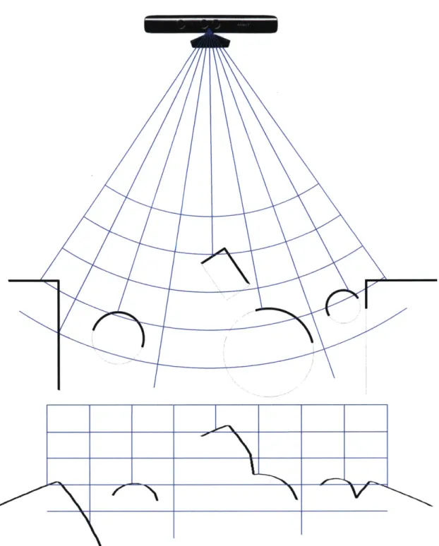
3-2 Warping spherical coordinates into rectangular coordinates. . . . . 61

3-3 Examples of object poses that are at the same rotation in spherical

coordinates. . . . . 63

3-4 An example of edges missed by an edge detector. . . . . 64

3-5 Normal distributions with and without a receptive field radius. ... 64

3-6 2D normal distributions with elliptical and circular covariances. . . 65

4-1 Examples of synthetic images. . . . . 69

4-2 Visualizations of enumerated features . . . . 74 4-3 The effect of varying the minimum distance between parts. . . . . 77

4-4 Different objects and viewpoints vary in the area of the image they cover. 78 4-5 The minimum distance between parts should not be the same for all

view s. . . . . 79

4-6 The PR2 robot with camera height and pitch angles. . . . . 83

5-1 Hough transforms for visual parts in 1D. . . . . 92

5-2 Adding a rotation dimension to figure 5-1. . . . . 93

5-3 Adding a scale dimension to figure 5-1. . . . . 94

5-4 Hough transforms for visual parts in 2D. . . . . 96

5-5 Hough transforms for depth parts in 2D. . . . . 97

5-6 The maximum of the sum of 1D Hough votes in a region. . . . . 103

5-7 The maximum of the sum of Hough votes with rotation in a region. . 104 5-8 The maximum of the sum of Hough votes with scale in a region is broken into parts. . . . . 105

5-9 The maximum of the sum of Hough votes in a region for optical char-acter recognition. . . . . 106

5-10 The maximum of of the sum of Hough votes for depth parts in 2D. . 107 5-11 ID Hough transform votes and bounding regions aligned to image co-ordinates. ... ... ... 108

5-12 Hough transform votes for visual parts (with rotation) and bounding regions aligned to image coordinates. . . . . 109

5-13 Hough transform votes for visual parts (with scale) and bounding re-gions aligned to image coordinates. . . . . 110

5-14 Hough transform votes for depth parts and bounding regions in warped coordinates. . . . . 111

5-15 1D Hough transform votes and bounding regions with receptive field radius. . . . . 114

5-16 Hough transform votes (with scale), bounding regions and receptive field radius. . . . . 115

5-17 Hough transform votes for depth parts with bounding regions and re-ceptive field radius. . . . . 118

6-1 Average Precision vs. Number of Training Images (n) . . . . 139

6-2 Average Precision vs. Number of Visual Parts (ny) . . . . 140

6-4 Average Precision vs. Number of Visual and Depth Parts (nD = nV) 142

6-5 Average Precision vs. Receptive Field Radius For Visual Parts (rv) 143

6-6 Average Precision vs. Receptive Field Radius For Depth Parts (rD) 144

6-7 Average Precision vs. Maximum Visual Part Variance (vvmax) . . . . 145

6-8 Average Precision vs. Maximum Depth Part Variance (VDmax) . . . . 146

6-9 Average Precision vs. Rotational Bin Width (r,) . . . . 147

6-10 Average Precision vs. Minimum Edge Probability Threshold . . . . . 148

6-11 Average Precision vs. Camera Height Tolerance (hto0) . . . . 149

6-12 Average Precision vs. Camera Pitch Tolerance (rtoi) . . . . 150

List of Tables

6.1 Detailed information about the objects and 3D mesh models used in

the experim ents. . . . . 136

6.2 Images of the objects and 3D mesh models used in the experiments. . 137 6.3 Parameter values used in experiments. . . . . 139

6.4 Average precision for each object, compared with the detector of Felzen-szw alb et al. [10]. . . . . 151

6.5 A confusion matrix with full-sized images. . . . . 152

6.6 A confusion matrix with cropped images. . . . . 152

6.7 Errors in predicted poses for asymmetric objects. . . . . 153

List of Algorithms

1 Render and crop a synthetic image. . . . . 69

2 Update an incremental least squares visual part by adding a new train-ing exam ple. . . . . 72

3 Finalize an incremental least squares visual part after it has been up-dated with all training examples. . . . . 72

4 Update an incremental least squares depth part by adding a new train-ing exam ple. . . . . 73

5 Finalize an incremental least squares depth part after it has been up-dated with all training examples. . . . . 73

6 Enumerate all possible features. . . . . 75

7 Select features greedily for a particular minimum allowable distance between chosen parts dmin. . . . . 78

8 Select features greedily for a particular maximum allowable part vari-ance vmax. . . . . 80

9 Learn a new viewpoint bin model. . . . . 81

10 Learn a full object model. . . . . 81

11 Evaluates a depth part for in image at a particular pose. . . . . 91

12 Evaluates a visual part for in image at a particular pose. . . . . 98

13 Evaluates an object model in an image at a particular pose. . . . . . 98

14 An uninformative design for a bounding function. . . . . 101

15 A brute-force design for a bounding function. . . . . 101

16 Calculate an upper bound on the log probability of a visual part for poses within a hypothesis region. . . . . 112

17 Calculate an upper bound on the log probability of a depth part for

poses within a hypothesis region by brute force. . . . 116

18 Calculate an upper bound on the log probability of a depth part for poses within a hypothesis region. . . . . 117

19 Calculate an upper bound on the log probability of an object for poses within a hypothesis region. . . . . 119

20 A set of high-level hypotheses used to initialize branch-and-bound search. 120 21 A test to see whether a point is in the constraint region. . . . . 122

22 Update the range of r, values for a pixel. . . . . 122

23 Find the range of r, values for a hypothesis region. . . . . 123

24 Update the range of r. values for a pixel. . . . . 123

25 Find the range of r. values for a hypothesis region. . . . . 124

26 Update the range of z values for a pixel. . . . . 125

27 Find the range of z values for a hypothesis region. . . . . 126

28 Find the smallest hypothesis region that contains the intersection be-tween a hypothesis region and the constraint. . . . . 126

29 One step in branch-and-bound search. . . . . 127

30 Detect an object in an image by branch-and-bound search. . . . . 127

31 Send a status update from a worker for parallel branch-and-bound. 129 32 A worker for a parallel branch-and-bound search for an object in an im age. . . . 130

33 Coordinate workers to perform branch-and-bound search in parallel. . 132

Chapter 1

Introduction

In this thesis we address the problem of finding the best 3D pose for a known object, supported on a horizontal plane, in a cluttered scene in which the object is not significantly occluded. We assume that we are operating with RGB-D images and some information about the pose of the camera. We also assume that a 3D mesh model of the object is available, along with a small number of labeled images of the object.

The problem is motivated by robot systems operating in indoor environments that need to manipulate particular objects and therefore need accurate pose estimates. This contrasts with other vision settings in which there is great variability in the objects but precise localization is not required.

Our goal is to find the best detection for a given view-based object model in an image, even though it takes time to search the whole space of possible object loca-tions. After searching, we guarantee that we have found the best detection without exhaustively searching the whole space of poses by using branch-and-bound methods. Our solution requires the user to have a 3D mesh model of the object and an RGB-D camera that senses both visual and depth information. The recent advances in RGB-D cameras have proven to give much higher-accuracy depth information than previous stereo cameras. Moreover, RGB-D cameras like the Microsoft Kinect are cheap, reliable and broadly available. We also require an estimate of the height and pitch angle of the camera with respect to the horizontal supporting plane (i.e.

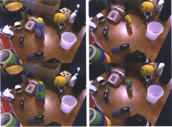
Figure 1-1: Examples of correct object detections. Detections include the full 6 dimensional location (or pose) of the object. The laundry detergent bottle (top left)

table) on which the upright object is located. The result is a 6 degree-of-freedom pose estimate. We allow background clutter in images, but we restrict the problem to images in which the object is not significantly occluded. We also assume that for each RGB-D image, the user knows the pitch angle of the camera and the height of the camera measured from the table the object is on.

This is a useful problem in the context of robotics, in which it is necessary to have an accurate estimate of an object's pose before it can be grasped or picked up. Although less flexible than the popular paradigm of learning from labeled real images of a highly variable object class, this method requires less manual labor-only a small number of real images of the object instance with 2D bounding box labels are used to test the view-based model and to tune learning parameters. This makes the approach practical as a component of a complete robotic system, as there is a large class of real robotic manipulation domains in which a mesh model for the object to be manipulated can be acquired ahead of time.

1.1

Overview of the Approach

Our approach to the problem is to find the global maximum probability object local-ization in the full space of rigid poses. We represent this pose space using 3 positional dimensions plus 3 rotational dimensions, for a total of 6 degrees of freedom.

There are two key components to our approach:

" learning a view-based model of the object and " detecting the object in an image.

A view-based model consists of a number of parts. There are two types of parts:

visual parts and depth parts. Visual parts are matched to edges detected in an image

by an edge detector. Each visual edge part is tuned to find edges at one of 8 discrete

edge angles. In addition, small texture elements can be used to define other kinds of visual parts. Visual parts do not have depth, and the uncertainty about their positions is restricted to the image plane.

Depth parts, on the other hand, only model uncertainty in depth, not in the image plane. Each depth part is matched to a depth measurement from the RGB-D camera at some definite pixel in the image. Thus we can think of the 1D uncertainty of depth part locations as orthogonal to the 2D uncertainty of image part locations.

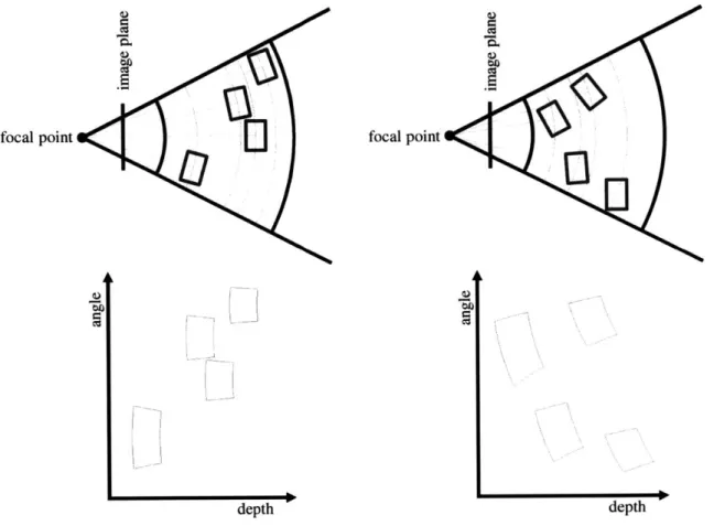
The expected position of each of the view-based model parts (both visual and depth parts) is a function of the object pose. We divide the 3 rotational dimensions of pose space into a number of viewpoint bins, and we model the positions of the parts as a linear function of the object rotation within each viewpoint bin (i.e. we use a small angle approximation). In this way, the position of the object parts is a piecewise linear function of the object rotation, and the domain of each of the "pieces" is a viewpoint bin. The 3 positional dimensions are defined with respect to the camera: as the object moves tangent to a sphere centered at the focal point of the camera, all the model parts are simply translated in the image plane. As the object moves nearer or farther from the camera, the positions of the parts are appropriately scaled with an origin at the center of the object (this is known as the weak perspective approximation to perspective projection). A view-based model consists of parts whose expected positions in the image plane are modeled by a function of all 6 dimensions of the object pose.

A view-based model is learned primarily from synthetic images rendered from a

mesh of the particular object instance. For each viewpoint bin, synthetic images are scaled and aligned (using the weak perspective assumption) and a linear model (using the small angle assumption) is fit to the aligned images using least squares.

An object is detected by a branch-and-bound search that guarantees that the best detections will always be found first. This guarantee is an attractive feature of our detection system because it allows the user to focus on tuning the learning parameters that affect the model, with the assurance that errors will not be introduced by the search process. A key aspect of branch-and-bound search is bounding. Bounding gives a conservative estimate (i.e. an upper bound) on the probability that the object is located within some region in pose space.

based on the part's position. These votes assign a weight to every point in the

6D space of object poses. The pose with the greatest sum of "votes" from all of

the parts is the most probable detection in the image. We therefore introduce a bounding function that efficiently computes an upper bound on the votes from each part over a region of pose space. The bounding function is efficient because of the weak perspective projection and small angle approximations. These approximations

allow the geometric redundancy of the 6D votes to be reduced, representing them in lower dimensional (2D and 3D) tables in the image plane. To further save memory and increase efficiency, these lower dimensional tables are shared by all the parts tuned to a particular kind of feature, so that they can be re-used to compute the bounding functions for all the parts of each kind.

1.1.1

Learning

Input: An instance of the object, a way to acquire a 3D mesh, an RGB-D camera with the ability to measure camera height and pitch angle

Output: A view-based model of the object, composed of a set of viewpoint bins, each with visual and depth parts and their respective parameters

We break the process of learning (described in depth in chapter 4) a new view-based model into two parts. First we will discuss the fully automated view-view-based model learning subsystem that generates a view-based model from a 3D mesh and a specific choice of parameter values. Then we will discuss the procedure required to tune the parameter values. This is a manual process in which the human uses the view-based learning subsystem and the detection system to repeatedly train and test parameter values. The model learning and the detection sub-procedures can be called

by a human in this manual process.

1.1.1.1 View-Based Model Learning Subsystem

Input: A 3D mesh and parameter values such as the set of viewpoint bins

bins, each with visual and depth parts along with the coefficients of the linear model for their positions and the uncertainty about those positions

The view-based model learning subsystem (see figure 1-2) is a fully automated process that takes a mesh and some parameter values and produces a view-based model of the object. This subsystem is described in detail in section 4.1. The position of each object part is a piecewise linear function of the three rotation angles about each axis. Each piece of this piecewise linear model covers an axis-aligned "cube" in this 3D space of rotations. We call these cubes viewpoint bins. 3D objects are modeled with a number of different viewpoint bins, each with its own linear model of the object's shape and appearance for poses within that bin. The following three learning phases are repeated for each viewpoint bin:

1. rendering the image,

2. enumerating the set of features that could be used as model parts,

3. selecting the features that will be used in the final viewpoint bin model and

4. combining viewpoint bin models into the final view-based model.

Since each viewpoint bin is learned independently, we parallelize the learning pro-cedure, learning each view-based model on a separate core. In our tests, we had nearly enough CPUs to learn all of the viewpoint bin models in parallel, so the total learning time was primarily determined by the time taken to learn a single viewpoint bin model. On a single 2.26 GHz Intel CPU core, learning time takes an average of approximately 2 minutes.

The view-based model learning subsystem is designed to be entirely automated, and require few parameter settings from the user. However, there are still a number of parameters to tune, as mentioned in section 1.1.1.2.

An unusual aspect of this learning subsystem is that the only training input to the algorithm is a single 3D mesh. The learning is performed entirely using synthetic images generated from rendering this mesh. This means that the learned view-based

model will be accurate for the particular object instance that the mesh represents, and not for a general class of objects.

Rendering

Input: a 3D mesh and parameters such as viewpoint bin size and ambient lighting

level

Output: a sequence of cropped, scaled, and aligned rendered RGB-D images for

randomly sampled views within the viewpoint bin

Objects are rendered using OpenGL at a variety of positions and rotations in the view frustum of the virtual camera, with a variety of virtual light source positions. This causes variation in resolution, shading and perspective distortion, in addition to the changes in appearance as the object is rotated within the viewpoint bin. The virtual camera parameters are set to match the calibration of the real Microsoft Kinect camera. The OpenGL Z-buffer is used to reconstruct what the depth image from the Microsoft Kinect would look like.1 Each of the images are then scaled and translated such that the object centers are exactly aligned on top of each other. We describe the rendering process in more detail in section 4.1.1.

Feature Enumeration

Input: a sequence of scaled and aligned RGB-D images

Output: a least squares linear model of the closest feature position at each pixel for

depth features and for each kind of visual feature

The rendered images are used to fit a number of linear functions that model how the position of each visual feature (such as edges) and depth value varies with small object rotations within the viewpoint bin. A linear function is fit at each pixel in the aligned images, and for each edge angle as well as for each pixel in the aligned depth images. The linear functions are fit using least squares, so the mean squared

'This method is only an approximate simulation of the true process that generates RGB-D images in the Kinect. For example, the real Kinect has a few centimeters of disparity between the infrared camera that measures depth and the color camera, so that the visual and depth images are not aligned at all depths.

depth edges (8 edge -67.50 -450 -22.5* 45* 6 viewpoint bin 1 0-0I

I

s)

.

depth edges (8 edge angles) 'M.& -77 ko n

22.5* 45* 67.5* 90* I .

fetr

enmraS

Figure 1-2: An overview of the view-based model learning subsystem. Random poses are sampled from within each view, and synthetic RGB-D images are rendered at these views. These images are then scaled and translated so that the centers of the objects in the images are aligned. Next, a linear model is fit at each pixel for each type of visual feature (8 edge directions in this figure) detected in the synthetic images, and another linear model is fit at each pixel for the depth measurements that come from the Z-buffer of the synthetic images. Finally, some of those linear models are selected and become parts of the final viewpoint bin model. Each of the 360 viewpoint bin models are combined to form piecewise linear segments of a full view-based model.

Note: this procedure does not take any real images as an input-the learned models will later be tested on real images.

error values are a readily available metric to determine how closely the models fit the actual simulated images.

In reality, feature enumeration is a process that occurs incrementally as each new rendered image is generated. This saves memory and greatly increases learning speed. We use a formulation of the least squares problem that allows each training point to be added sequentially in an online fashion.

The speed of this process could be improved by the fine-grained parallelism avail-able on a GPU architecture, computing the feature enumeration for each pixel of each kind of feature in parallel.

We give more details in section 4.1.2.

Feature Selection

Input: a set of linear models for positions of each kind of feature at each pixel and

parameter values for how visual and depth parts should be modeled

Output: a model for a viewpoint bin, consisting of a selection of these part models

with low mean-squared-error and spaced evenly across the image of the viewpoint From the set of enumerated features, a small fixed number are selected to be parts of the model for the viewpoint bin. They are greedily chosen to have a low mean squared error, and even spacing across the image of the viewpoint bin model. Most of the user-specified learning parameters are used to control this stage of the learning process. The selected parts constitute the model for each particular viewpoint bin, and the set of viewpoint bins form the whole object model. We provide more details in section 4.1.3.

Combining Models Of Viewpoint Bins

Input: a set of object models for all the different viewpoint bins

Output: an view-based model covering the region of pose space covered by the union

of the input viewpoint bins

A view-based model consists of a set of viewpoint bin models, each of which has

viewpoint bin models are grouped together to form the complete view-based model. We give more details in section 4.1.4.

1.1.1.2 High Level Learning Procedure

Input: An instance of the object, a way to acquire a 3D mesh, an RGB-D camera

with the ability to measure camera height and pitch angle and computational power.

Output: A view-based model of the object, composed of a set of viewpoint bin

models, each with visual and depth parts

The procedure to learn a new view-based model is depicted in figure 1-2. The steps involved are:

1. Collect RGB-D images of the object, along with information about the camera

pose, and partition the images into a test and hold-out set. 2. Label the images with bounding boxes.

3. Acquire a 3D mesh of the object (usually by 3D scanning).

4. Tune learning parameters while testing the view-based models on the test im-ages.

5. Evaluate the accuracy of the view-based models.

We describe this procedure in section 4.2.

Collect RGB-D Images Input:

* the object instance,

e the object instance, placed on a table and

* an RGB-D camera with the ability to measure the table,

"""""""pararaeterr

collect images & data using

a PR2 robot with a inect

labe

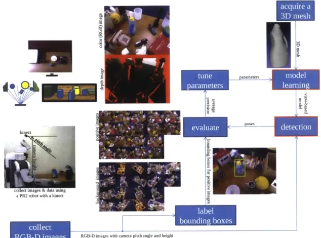
Figure 1-3: An overview of the manual labor required to learn a new object. To learn a new view-based model of an object, we first collect a data set of about 30 positive image examples of the object and about 30 background images of the object (all images used for training the downy bottle view-based model are in this figure). Each image must also include the pitch angle of the camera and the height of the camera above the table when the image was taken. The images should also include depth information. We use a PR2 robot with a Microsoft Kinect mounted on its head to gather our data sets. Each positive example must be labeled by a human with an approximate 2D bounding box for the object to detect. A 3D mesh of the object should be acquired (usually using a 3D scanner). The mesh is used to learn a new view-based model, and the learning parameters must be manually adjusted as the user tests each new learned view-based model on the real images and evaluates the accuracy (measured by average precision).

Output: a set of RGB-D images labeled with the camera's pitch and its height above

table

In our experiments, we collect a set of around 15 images with depth information (RGB-D images) for each object using a Microsoft Kinect mounted on a PR2 robot. In our data sets, we did not manually change the scene between each image capture-we set up a table with background clutter and the object one time, and capture-we drove the robot to different positions around the table, ensuring that the object was not occluded in any images, since our detector does not currently deal explicitly with occlusion. This process took about 10 minutes per object. The reason we used the robot instead of manually holding the Kinect camera and walking around the table is that we also record the camera height above the table and its pitch (assuming the camera is upright and level with ground, i.e., the roll angle of the camera in the plane of the image is always zero). An affordable alternative to this method would be to instrument a tripod with a system to measure the camera's height and pitch. This information is used to constrain the 6D search space to search a region surrounding the table, at object rotations that would be consistent (or nearly consistent) with the object standing upright on the table.

We also collected a set of about 15 background images that contained none of the objects we were interested in detecting using this same methodology. We were able to re-use this set of images as negative examples for each of the objects we tested.

Label Bounding Boxes Input: a set of RGB-D images

Output: left, right, top and bottom extents of an approximate rectangular bounding

box for each image of the object

We use a simple metric to decide whether a detection is correct: if the 2D rectangle that bounds the detection in the image plane overlaps with the manually-labeled bounding box according to the standard intersection over union (IoU) overlap metric

of the detected bounding box A and the ground truth bounding box B:

AuB> 0.5 _(1.1)

This leaves some room for flexibility, so the labeled bounding boxes do not need to be accurate to the exact pixel. Labeling approximate bounding boxes for a set of about

30 images takes around 10 minutes for a single trained person.

We labeled our image sets with 6D poses for the purposes of evaluating our algo-rithm in this thesis. However, we found that, even if we know the plane of the table from the camera height and pitch angle, labeling 6D poses is very time-consuming, difficult and error-prone, so we decided to reduce the overall manual effort required of the end user by relaxing the labeling task to simple bounding boxes.

We suggest that, in practice, the accuracy of detected poses can be evaluated directly by human inspection, rather than using full 6D pose labels.

Acquire A 3D Mesh Input: the object instance

Output: an accurate 3D mesh of the object instance

We found that the accuracy of the detector is highly related to the accuracy of the 3D mesh, so it is important to use an accurate method of obtaining a mesh. The scanned mesh models used in this thesis were mostly obtained from a commercial scanning service: 3D Scan Services, LLC. Some of the mesh models we used (such boxes and cylinders) were simple enough that hand-built meshes yielded reasonable accuracy.

Tune Parameters Input:

results of evaluating the view-based object detector

a sample of correct and incorrect detections from the view-based model learned from the previous parameter settings

Output: a new set of parameter values that should improve the accuracy of the

view-based model

There are many learning parameters involved in producing a view-based model, such as:

" the size of the viewpoint bin,

* the amount of ambient lighting in the rendered images,

* the maximum allowable mean squared error in feature selection, etc.

It would be computationally infeasible to test all combinations of parameter settings to automatically find the best-performing values, so this is left as a manual process.

A human can look at a visualization of a view-based model, and the set of detections

for that model, and see where the pattern of common failure cases are. A bit of intuition, experience and understanding of how the view-based model is constructed can help the human to make educated guesses as to which parameters need to be adjusted to improve the performance. For example, by looking at a visualization of a view-based model, one may realize that the set of view bins does not fully cover the set of object rotations in the real world, so the user would adjust the set of viewpoint bins and re-run the learning and test to see if it performs more accurately. Or the user may notice that there appear to be randomly scattered edge parts in the view-based model. In this case, the user may try to reduce the maximum allowable mean squared error for edge feature selection.

This is admittedly the most difficult part of the process, as it requires a fair amount of experience. Section 4.2.1 gives more details on our methodology and chapter 6 gives a sample of the kinds of experiments that we used to determine good parameter settings, but the real process involves some careful inspection of detections, an understanding of how the view-based model is affected by the parameters, and

some critical thinking.

Input:

" a set of detected object poses in images,

" hand-labeled bounding boxes for the object in the images, " a set of about 15 RGB-D images not containing the object

Output: a score between 0 and 1 evaluating the accuracy of the view-based model

on the set of test images

Since we only require 2D bounding box labels (to save manual labor), we are able to evaluate the accuracy of results following the standard and accepted methodology defined by the PASCAL [8] and ImageNet [29] challenges. The challenge defines correct detection with respect to the ground truth label by the intersection over union (IoU) metric (see section 1.1.1.2), and the overall detection accuracy on a set of test images is measured by an average precision that is a number between 0 and

1, where 1 represents perfect detection.

1.1.2

Detection

Input:

" An RGB-D image along with the camera height and the camera pitch angle " A view-based model

Output: A sequence of detected poses, ordered by decreasing probability that the

object is at each pose

The detection algorithm uses branch-and-bound search to find detections in de-creasing order of probability.

Branch-and-bound search operates by recursively breaking up the 6D search space into smaller and smaller regions, guided by a bounding function which gives an over-estimate of the maximum probability that the object may be found in a particular

region. Using the bounding function, branch-and-bound explores the most promising regions first, so that it can provably find the most probable detections first.

The bounding function in branch-and-bound search is the critical factor that de-termines the running time of the search process. The. over-estimate of the bound should not be too far above the true maximum probability (i.e. the bound should be tight), and time to compute the bound should be minimal. In our design of the detection algorithm, computational efficiency of the bounding function is the primary consideration.

The detection algorithm consists of five steps:

1. detect visual features

2. pre-process the image to create low-dimensional tables to quickly access the 6D search space

3. initialize the priority queue for branch-and-bound search

4. run the branch-and-bound search to generate a list of detections

5. suppress detections that are not local maxima to remove many redundant

de-tections that are only slight variations of each other Chapter 5 gives more details about the detection algorithm.

Visual Feature Detection Input: an RGB-D image

Output: a binary image of the same dimensions, for each kind of visual feature The first phase of detection is to detect the low-level features. Depth

measure-ments are converted from Euclidean space, into measuremeasure-ments along a 3D ray starting at the focal point of the camera passing through each pixel. Visual features must be extracted from the input image. Visual feature detectors determine a binary value of whether the feature is present, or absent at any feature. In this thesis, we use an edge detector to extract edge pixels from an edge detector from around 8 different edge directions. We provide more details in section 5.2.

depimage(1D slice of 2D)

Lr . l1_

RGB/visual image (1D slice of 2D)

-"" summed area table of depth (21) slice of 3D) summed area tables of visual features (ID slice of 2D)

distance transforms of visual features

summed area tables and distance transforms

F

I

I

O

I

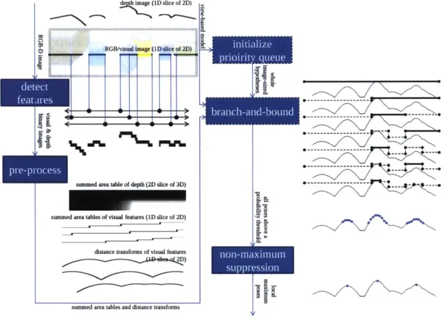
Figure 1-4: An overview of detection. First features are detected in the image, then these binary feature images are preprocessed to produce summed area tables and distance transforms. The priority queue used in the branch-and-bound search is initialized with a full image-sized region for each viewpoint bin. As branch-and-bound runs, it emits a sequence of detections sorted in decreasing order of probability. Some of these detections that are redundantly close to other, higher-probability detections are then removed (or "suppressed").

-

Ili t

rM6WM

=. $0

Pre-processing

Input: a depth image and a binary image of the same dimensions, for each kind of

visual feature

Output:

" a 3D summed area table computed from the depth image

" a 2D summed area table computed from each kind of visual feature

" a 2D distance transform computed from each kind of visual feature

Before the process of searching for an object in an image begins, our algorithm builds a number of tables that allow the bounding function to be computed efficiently. First, edges are detected in the image. Each edge has an angle, and edges are grouped into 8 discrete edge angle bins. Each edge angle bin is treated as a separate feature. An optional texture detection phase may be used to detect other types of visual features besides edges. 2D binary-valued images are created for each feature, recording where in the RGB-D image the features were detected, and where they were absent.

The bounding function needs to efficiently produce an over-estimate of the maxi-mum probability that the object is in a 6D region in pose space. A dense 6D structure table would be large, and even if it could fit in RAM, it would be slow because the whole structure could never fit in the CPU cache. We therefore store 2D and 3D tables that are smaller in size and more likely to fit in a CPU cache for fast read access.

Each feature in the image has a maximum receptive radius, which is the region of pose space where it may increase the overall "votes" for those poses. A feature can have no effect on the total sum of votes for any pose outside of its receptive field radius. The key idea of the bounding function for a particular part is to conservatively assume the highest possible vote for that feature for a region of pose space that may intersect the receptive field radius of some feature. Otherwise, it is safe to assume the lowest possible vote for that region. To make the bounding function efficient, we

take advantage of a property of a summed area table [6] (also known as an integral image [36]) that allows us to determine whether a feature is present in any rectangular region with a small constant number of reads from the table. A separate 2D summed area table is used for each visual feature (such as each edge angle). We similarly compute a 3D summed area table for depth features. The constant access time property of the summed area table means that the bounding function takes the same amount of time to compute, regardless of how big or small the region is.

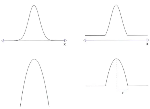
We would also like to efficiently compute the exact probabilities when branch-and-bound arrives at a leaf of the search tree. The uncertainty of visual feature locations are modeled by normal distributions in the image plane. The logarithm of a normal distribution is simply a quadratic function (i.e. a parabola with a 2D domain), which is the square of a distance function. To find the highest probability match between a visual part and a visual feature in the image (such as an edge), we want to find the squared distance to the visual feature that is closest to the expected location of the part. A distance transform is a table that provides exactly this information-it gives the minimum distance to a feature detection at each pixel [11]. A distance transform is pre-computed for each kind of visual feature so that any the exact probability of any visual part can be computed with only one look-up into the table for the appropriate kind of visual feature.

We underscore that these pre-computed tables are shared for all parts of a par-ticular kind. In other words, the total number of pre-computed tables in memory is proportional to the number of different kinds features (usually 8 discrete edge di-rections), which is many fewer than the number of parts in a viewpoint bin model (usually 100 visual and 100 depth parts), or the number of viewpoint bin models or even the number of different object types being detected. This contributes to a significant increase in search efficiency.

These tables take about 4 seconds to compute on a single core 2.26 GHz Intel

CPU.

Input: an empty priority queue, and the viewpoint bin sizes of the view-based model Output: a priority queue containing a maximum-size region for each viewpoint bin,

each with its appropriate bound

Besides the tables used to compute the bounding function discussed in the last chapter, the other major data structure used by branch-and-bound search is a priority

queue (usually implemented by a heap data structure). The priority queue stores the

current collection of working hypothesis regions of pose space, prioritized by their maximum probability. The priority queue is designed to make it efficient to find and remove the highest-priority (maximum probability bound) region. It is also fast to

add new regions with arbitrary bounds onto the priority queue.

Branch-and-bound search starts with the initial hypothesis that the object could be anywhere (subject to the current set of constraints, such as whether it is near a table top). We therefore put a full-sized region that covers the whole 6D pose space we are considering for each viewpoint bin on the priority queue. These initial regions are so large that they are uninformative-the bounding function will give a very optimistic over-estimate, but it will still be fast to compute since the running

time does not vary with the size of the region.

Initializing the priority queue takes a negligible amount of time.

Branch-and-Bound Search Input: an initialized priority queue

Output: the sequence detections (i.e. points in pose space) sorted in descending

order of probability that the object is located there

Branch-and-bound search removes the most promising hypothesis from the prior-ity queue and splits it into as many as 26 "branch" hypotheses because there are 6 dimensions in the search space. It computes the bounding function for each branch, and puts them back onto the queue. When it encounters a region that is small enough, it exhaustively tests a 6D grid of points within the region to find the maximum prob-ability point, and that point is then pushed back onto the priority queue as a leaf. The first time that a leaf appears as the maximum probability hypothesis, we know

that we have found the best possible detection.

As we have said, the bounding function is the most critical factor in the efficiency of the branch-and-bound search process. Inherent in the design of our view-based model representation are two approximations: weak perspective projection and the small-angle approximation. These two approximations make the bounding function simple to compute using the low dimensional pre-computed tables (discussed in section 1.1.2).

These approximations make it possible to access these low-dimensional tables in a simple way: using only scaling and translations, rather than complex perspective functions or trigonometric functions. A rectangular 6D search region can be projected down to a 2D (or 3D) region, bounded by a rectangle in the pre-computed summed area tables, with some translation and scaling. This region can then be tested with a small constant number of reads from these tables in constant time for each visual and depth part.

The leaf probabilities can also be computed quickly by looking up values at ap-propriately scaled and translated pixel locations in the distance transforms for each kind of visual feature, and scaling and thresholding those distances values according to the parameters of each part.

We tested the detection algorithm on 20 2.26 GHz Intel 24-core machines in par-allel, each 24-core machine had 12 GB of RAM. Under these conditions, this process usually takes about 15-30 seconds. The search procedure is parallelized by giving each processor core its own priority queue to search its own sub-set of the pose search space. When a priority queue for one core becomes empty, it requests more work, and another core is chosen to delegate part of its priority queue to the empty core.

If searching for only the best n detections, then the current nth best probability is

continually broadcasted to all of the CPUs because any branches in the search tree with lower probability can be safely discarded. At the end of the search, the final set of detections are collected and sorted together.

The speed of this process could be improved by the fine-grained parallelism avail-able on a GPU architecture, by computing the "vote" from each of the object parts in parallel. Under this strategy, the memory devoted to the priority queue would be

located on the host CPU, while the memory devoted to the read-only precomputed tables would be located on the GPU for faster access. The amount of communication between the GPU and the CPU would be low: only a few numbers would be trans-ferred at evaluation of a search node: the current search region would be sent to the

GPU, and the probability of that region would be returned to the CPU. This means

the problem would be unlikely to suffer from the relatively low-bandwidth connection between a CPU and a GPU.

Non-Maximum Suppression

Input: a list of detections with their corresponding probabilities

Output: a subset of that list that only keeps detections whose probabilities are a

local maximum

If branch-and-bound search continues after the first detection is found, the

se-quence of detections will always be in decreasing order of probability. In this sese-quence of detections, there are often many redundant detections bunched very close to each other around the same part of the pose space.

In order to make the results easier to interpret, only the best detection in a local region of search space is retained, and the rest are discarded. We refer to this process as non-maximum suppression.

Non-maximum suppression takes a negligible amount of computation time.

1.2

Outline of Thesis

In chapter 2 we discuss related work in the field of object recognition and situate this thesis in the larger context. In chapter 3, we give the formal representation of the view-based model we developed. Chapter 4 describes how we learn a view-based model from a 3D mesh model and from images. Chapter 5 describes our algorithm for detecting objects represented by a view-based model in an RGB-D image. Chapter 6 describes our experiments and gives experimental results. Finally, chapter 7 discusses the system and gives conclusions and directions for future work.

Chapter 2

Related Work

In this chapter, we give a brief overview of some of the work in the field of object recognition that relates to this thesis. For an in-depth look at the current state of the entire field of object recognition, we refer the reader to three surveys:

" Hoiem and Savarese [18], primarily address 3D recognition and scene

under-standing.

" Grauman and Leibe [16] compare and contrast some of the most popular

ob-ject recognition learning and detection algorithms, with an emphasis on 2D algorithms.

" Andreopoulos and Tsotsos [2], examines the history of object recognition along with its current real-world applications, with a particular focus on active vision.

2.1

Low-Level Features

Researchers have explored many different low-level features over the years. Section

4.3 of Hoiem and Savarese [18] and chapter 3 of Grauman and Leibe [16] give a good

overview of the large number of features that are popular in the field such as SIFT [25] or HOG [7] descriptors. In addition to these, much recent attention in the field has been given to features learned automatically in deep neural networks. Krizhevsky et

al. [21] present a recent breakthrough work in this area which is often referred to as deep learning. In this thesis, we use edges and depth features.

Edges are useful because they are invariant to many changes in lighting conditions. One of the most popular edge detectors by Canny [3] is fast-it can detect edges in an image in milliseconds. More recent edge detectors like that of Maire et al. [26] achieve a higher accuracy by using a more principled approach and evaluating accuracy on human-labeled edge datasets-however these detectors tend to take minutes to run on a single CPU'. With the advent of RGB-D cameras and edge datasets, the most recent edge detectors such as the one by Ren and Bo [28] have taken advantage of the additional information provided by the depth channel. We use the Canny [3] and Ren and Bo [28] edge detectors in our experiments.

Although the computer vision research community has traditionally focused on analyzing 2D images, research (including our work in this thesis) has begun to shift towards making use of the depth channel in RGB-D images. In this thesis, we also use simple depth features: at almost every pixel in an RGB-D image, there is a depth measurement, in meters, to the nearest surface intersected by the ray passing from the focal point of the camera through that pixel (however, at some pixels, the RGB-D camera fails, giving undefined depth measurements).

2.2

Generic Categories vs. Specific Objects

We humans can easily recognize a chair when we see one, even though they come in such a wide variety of shapes and appearances. Researchers have primarily focused on trying to develop algorithms that are able to mimic this kind of flexibility in object recognition-they have developed systems to recognize generic categories of objects like airplanes, bicycles or cars for popular contests like the PASCAL [8] or ImageNet recognition challenges [29]. In addition to the variability within the class, researchers have also had to cope with the variability caused by changes in viewpoint and lighting. The most successful of these algorithms, such as Felzenszwalb et al. [10],

Viola and Jones [36] and Krizhevsky et al. [21] are impressive in their ability to locate and identify instances of generic object classes in cluttered scenes with occlusion and without any contextual priming. These systems usually aim to draw a bounding box around the object, rather than finding an exact estimate of the position and rotation of the object. They also usually require a large number of images with hand-labeled annotations as training examples to learn the distribution of appearances within the class. Image databases such as ImageNet [29], LabelMe [30] and SUN [37] have been used to train generic detection systems for thousands of objects.

In this work, we, along with some other researchers in the field, such as Lowe [25], and Nister and Stewenius [27] have chosen to work on a different problem-recognizing an object instance without class variability, but requiring a more accurate pose es-timate. Setting up the problem in this way rules out all of the variability from a generic class of objects. For example, instead of looking for any bottle of laundry detergent, these algorithms might specifically look for a 51 fl. oz. bottle of Downy laundry detergent manufactured in 2014. Although within-class variability is elimi-nated by simplifying the problem, there is still variability in shape and appearance from changing viewpoints and lighting. Chapter 3 of Grauman and Leibe [16] dis-cusses a number of local feature-based approaches that have been very successful in detecting and localizing specific object instances with occlusion in cluttered scenes using only a single image of the object as a training example. But these approaches usually require the objects to be highly textured, and their accuracy tends to decrease with large changes in viewpoint.

2.3

2D vs. 3D vs. 21D view-based models

Hoiem and Savarese [18] divide view-based object models into three groups: 2D, 3D and 21D.

2.3.1

2D view-based models

Researchers have used a variety of different 2D object representations. If the object class is like a face or a pedestrian that is usually found in a single canonical viewpoint, then it can be well represented by a single 2D view-based model. Two of the most popular techniques for detecting a single view of an object are rigid window-based templates and flexible part-based models.

Window-based models

One search strategy, commonly referred to as the sliding window approach, compares a rigid template (a "window") to every possible position (and scale) in the scene to detect and localize the object. Viola and Jones [36] demonstrated a very fast and accurate face detector, and Dalal and Triggs [7] made a very accurate pedestrian detector using this technique. More recently, Sermanet et al. [31] have successfully used the deep learning approach in a sliding window strategy, and Farfade et al. [9] have shown that this kind of strategy can even be robust to substantial variations in poses. However, window-based methods have primarily been used for object detection

and have not yet been demonstrated to localize precise poses.

Part-based models

In order to detect and localize objects in a broader range of viewpoints, the view-based model may need to be more flexible. A common way of adding flexibility is to modularize the single window template by breaking it into parts. Each part functions as a small template that can be compared to the image.

Several different representations have been used to add flexibility in the geometric layout of these parts relative to each other. Lowe [25] used an algorithm called

RANSAC (invented by Fischler and Bolles [14]) to greedily and randomly match

points to a known example (see section 2.4.1).

Another technique is to represent the layout of the parts as if they were connected