3-D hybrid Eulerian-Lagrangian / particle tracking model for simulating mass transport in coastal water bodies

(1)

3-D HYBRID EULERIAN-LAGRANGIAN / PARTICLE TRACKING

MODEL FOR SIMULATING MASS TRANSPORT IN COASTAL

WATER BODIES

by

Konstantina Dimou

Diploma, National Technical University, Athens

(1987)

S.M., Massachusetts Institute of Technology

(1989)

Submitted to the Department of Civil Engineering in partial fulfillment of the requirements

for the degree of

DOCTOR OF PHILOSOPHY at the

MASSACHUSETTS INSTITUTE OF TECHNOLOGY

May, 1992

( Massachusetts Institute of Technology 1992

ACHIVES

MASSACHUSETS INSTITUTE rF TrCe4Nl.OGY JUN 3 0 1992 UBHAtIES Signature of Author

Department of Civil Engineering

May 15, 1992

Certified by

E. Eric Adams Lecturer, Department of Civil Engineering

'/?

Thesis Supervisor

Accepted by _

Eduardo Kausel Chairman, Departmental Committee on Graduate Students

(2)

3-D Hybrid

Eulerian-Lagrangian / Particle Tracking Model

for Simulating Mass Transport

in Coastal Water Bodies

by

Konstantina Dimou

Submitted to the Department of Civil Engineering on May 15, 1992, in partial fulfillment of the

requirements for the degree of Doctor of Philosophy

Abstract

The purpose of this research is the development and analysis of a three-dimensional finite-element Eulerian-Lagrangian / particle tracking model for the simulation of passive pollutant transport in coastal areas. Particular emphasis is given on the sim-ulation of pollution sources (e.g. outfalls) whose spatial extend is small compared to that of the domain discretization. A hybrid particle tracking / Eulerian-Lagrangian method is developed and analyzed for the simulation of small scale sources: Mass discharge from the source is modeled by the release of particles. When the standard deviation of the particle distribution reaches a length scale of the order of the grid scale particle locations are mapped onto node concentrations and the calculations proceed in the Eulerian-Lagrangian mode. A technique for the interfacing of the par-ticle tracking mode and the Eulerian-Lagrangian mode is developed. The developed method for the simulation of sources is applied for the simulation of outfalls in coastal water problems. The issue of consistently modeling the intermediate flow field around the diffuser is investigated. In order to demonstrate the performance of the developed model it is applied in Massachusetts Bay.

Thesis Supervisor: E. Eric Adams Title: Lecturer

(3)

Acknowledgments

I am most thankful to my advisor Dr. E. Eric Adams for his constant help and support and for the educational opportunity, that he provided me. My sincere thanks goes to Professor Antonio M. Baptista and Professor Donald R. F. Harleman for their direction and many helpful suggestions through this work.

The Parsons Lab has been a most enjoyable work place. Pat Dixon takes all the praise for creating this warm environment. I especially thank my friends at the Lab Hari, Shawn and Maria, Nalin, John, Paul, Kaye, Lynn and Fernando for their support particularly during the last difficult months.

I would like to thank my sister, Christina, for undertaking these overseas trips, whenever I needed her presence. It is never easy to combine life at MIT with family life. To my husband, Kostas, who has seen me through five years at MIT from my first day here, I give my love and thanks and wish him success in his academic endeavors.

And to my parents Xenophon and Sia Dimou, words fall too short of expressing my appreciation. I hope that my son, George, will be as proud of me as I am of them.

This research was supported by the MIT Sea Grant College Program, National Oceanic and Atmospheric Administration, US Dept. of Commerce under Grant NA90AA-D-SG424.

(4)

...

100 ...

100

· . . 100 . . . 104

...

107

114 114 117 121 123 126 136 137 141 141 143 149 153 155 155 157 3-D 3 66

(6)

5.5 REFERENCES ... 159

6 Representation of Sea Outfalls - Application in Massachusetts Bay 161 6.1 Background ... 161

6.1.1 Methodology ... 164

6.1.2 Specification of length scale L of the intermediate flow field . . 175

6.2 Testing of the Model in Massachusetts Bay ... 176

6.2.1 General ... 176

6.2.2 Grid ... 178

6.2.3 Application to the NOMES Experiment ... 178

6.2.4 Demonstration - Application in Massachusetts Bay ... 208

6.3 Discussion ... ... 212

6.4 REFERENCES ... 227

7 Summary - Future Work 230 7.1 Summary ... 230

7.2 Future Work . . . ... 231

(7)

List of Figures

1-1 Modeling of Coastal Processes ... 15

2-1 QUICK scheme.(a) Control volume approach. (b) Quadratic upstream interpolation for cl, °) c, ), (from Leonard, 1979) (Substitute

1

with c in the figures ... 30

2-2 Stability range for QUICKEST scheme a =

t

C

Cu

= t 31 2-3 Illustration of the backwards method of characteristics. ... 35

2-4 Cartesian-Coordinate System ... 38

2-5 Three coordinate systems ... 41

2-6 Pathway of Advective Salinity Transport Originating from Point A after 2 Time Steps. (from Leendertsee, 1990). ... 45

2-7 Eulerian-Lagrangian approach for coupling the HM with the TM. . . 58

3-1 Boundary Conditions in Transport Problem ... 67

3-2 Definition of timesteps for different solution phases ... 71

3-3 ItTM vs. error = dv and Edif (from Baptista, 1985) . ... 76

34 nd vs E.dv (a)ead, dominates. (b) Etd dominates. (from Zhang, 1990) 77 3-5 Flowchart of Backtracking Algorithm ... 80

3-6 Searching method. ... 81

3-7 Slippery zone ... 83

3-8 Prismatic Triangular Quadratic Finite Element . ... 85

3-9 Pure rotation of a Gaussian cloud at z = 0 at time t = 3000 with At = 3000 (no numerical error) ... 87

(8)

3-10 Pure rotation of a Gaussian cloud at z = 0 at time t = 3000 with

At = 1000 (a) concentation field (b) absolute numerical error ... 88

3-11 Pure rotation of a Gaussian cloud at z = 0 at time t = 3000 with At = 100 (a) concentation field (b) absolute numerical error ... 89

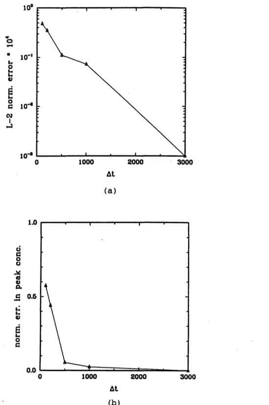
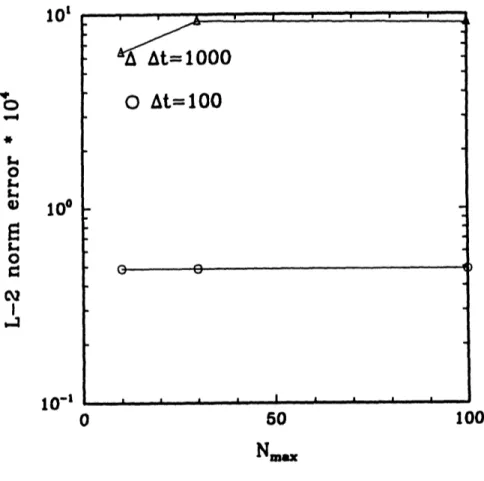
3-12 (a) L-2 error vs At (b) error in peak concentration vs At for Pe = oo. 90 3-13 (a) L-2 error vs At (b) error in peak concentration vs At for Pe = 57. 91 3-14 (a) L-2 error vs At (b) error in peak concentration vs At for Pe = 24. 92 3-15 L-2 error vs. Nm,,, using the 2nd order Runge Kutta method. .... 94

3-16 L-2 error vs. N,,a using the 5th order Runge Kutta method ... 95

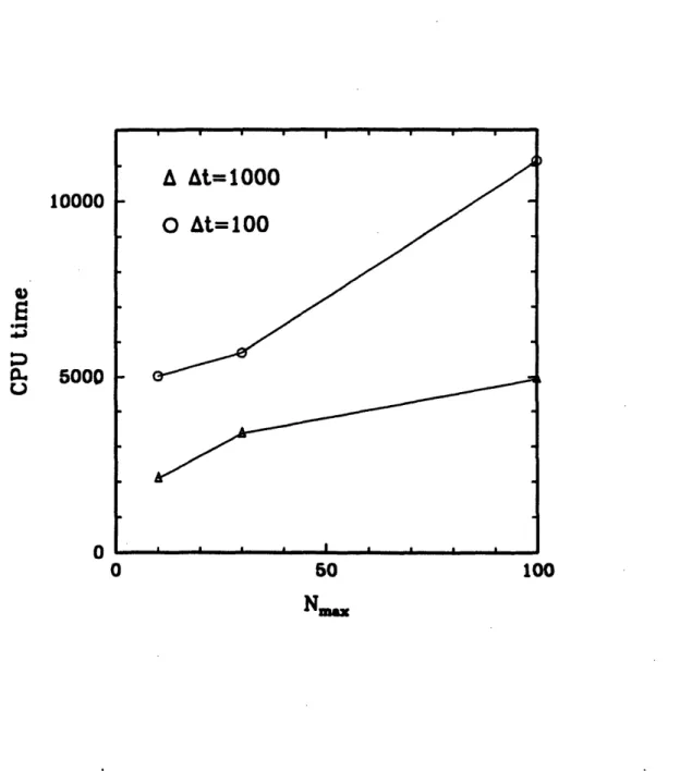
3-17 CPU (sec) in a DEC-3000 workstation vs. N,,a, using the 2nd order Runge Kutta method. ... 96

3-18 CPU (sec) in a DEC-3000 workstation vs. N using the 5th order Runge Kutta method. ... 97

3-19 Convergence rate of the diagonal preconditioner. ... 108

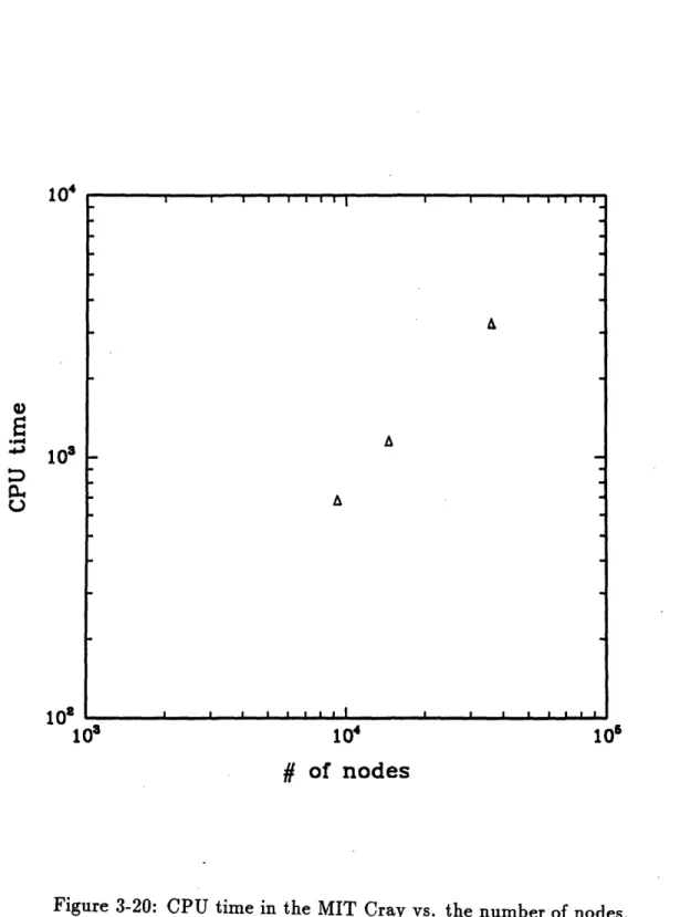
3-20 CPU time in the MIT Cray vs. the number of nodes. ... 109

4-1 Representation of sources. ... 119

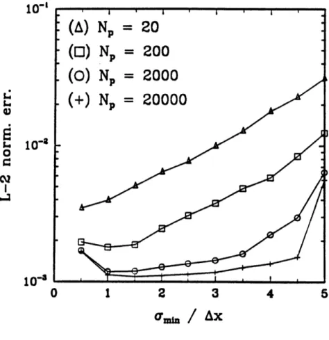
4-2 Comparison between a concentration model (A) and the developed hy-brid model (O ); solid line represents the mean concentrations; dashed lines represent the mean concentratins standard deviation for 50 Monte Carlo runs in a 1-D case (O = 2, t = 500,a mi. = 8) Axgrid = 1 125 4-3 Discrete normalized L-2 error vs. oami,/Axgrid in 1-D case for Np = 20 (A), Np = 200 ( o), Np = 2000 (x) and Np = 20000 (). Ensemble average values of 50 Monte Carlo simulations. ... 127

4-4 Normalized error in the peak concentration vs. amin//AXgrid in 1-D case for Np = 20 (A), Np = 200 ( o), Np = 2000 (x) and Np = 20000 (O). Ensemble average values of 50 Monte Carlo simulations. .... 128

(9)

4-5 Discrete normalized L-2 error vs. i,,i/,,Agrid in 1-D case for (a) Np

= 20 (A) (b) Np = 200 ( o), (c) Np = 2000 (x) and (d) p = 20000

( ). Ensemble average values ± standard deviation of 50 Monte Carlo

simulations ... 129

4-6 Amplification factor A vs. -L for the pure diffusion case using the first order Euler backwards scheme in time and quadratic finite elements in space (p = ) ... 131

4-7 Fourier Transform of the Gaussian distribution ... 132

4-8 Discrete normalized L-2 error vs. m,i,n/Agrid _{in a 3-D case for Np =} 200 ( o), Np = 2000 (x) and Np = 20000 (). ... 134

4-9 Normalized error in the peak concentration vs. oamin/Axgrid in a 3-D case for N = 200 ( o), N = 2000 (x) and N = 20000 (). ... 135

5-1 Representation of sources. ... 146

5-2 Projection functions. . . . 151

5-3 Types of ¢ functions (from Bagtzoglou, 1991). ... 152

5-4 Error in peak concentration vs. Np for a) dev = 2Agrid , b) dev = 4Axgrid and c) dev = 15AXgrid using Method A (o),Method B1 (x), Method C1 (l). ... 154

5-5 Discrete normalized L-2 error vs. Np using Methods B1 (thin line x), B2 (thin line ), C1 (bold line x) and C2 (bold line El) basis functions. (a)sd&, = 2Axgrid, (b) Sdev = 4AXgrid ... . . . . .. 156

5-6 Error in peak concentration vs. the grid irregularity parameter b for Np = 2000 using Methods A(thin line o), B1 with = AXb (thin line x), B1 with = Aa (bold line x) and C1 (thin line ) with linear basis functions ... ... 158

6-1 Near Flow Field. ... .... 162

6-2 Influence of ambient current on Si, and ztr (from Roberts et al, 1989). 166 6-3 Potential Flow solution for multiport diffuser. ... 168

(10)

6-5 Horizontal crossection of grid. . . . 171

6-6 Density Field at y = 0. . ... ... 172

6-7 Vertical profile of velocity at x = -4000 y = 0 ... 173

6-8

Vertical

profile

of

ambient

fluid

density

field.

... 174

6-9 Specification of length scale L of the intermediate flow field(from Hel-frich and Battisti) ... 177

6-10 Massachusetts Bay Grid (a bold line is used for the open boundary).. 179

6-11 NOMES experiment. The discharge point (E) and Station 5 are depicted. 181 6-12 Variation of w and over a tidal period . ... 183

6-13 Tidally-driven flow field (bottom) . . . 184

6-14 Tidally-driven flow field (z = -10m middepth) . ... 185

6-15 Tidally-driven flow field at the vicinity of the outfall (z = -10m mid-depth) ... 186

6-16 Tidally-driven flow field (surface) ... 187

6-17 Steady baroclinic flow field at the vicinity of the outfall (z = -10m

middepth).

...

.

188

6-18 Steady baroclinic flow field (middepth) for N = 0.2 . ... 190

6-19 Steady baroclinic flow field (middepth) for N = 0.002. ... 191

6-20 Steady baroclinic flow field (vertical profile of horizontal velocities) for N = 0.02. (a) k = 0.5, (b) k = 0.005 . ... 192

6-21 Current data at station 5 and HM results for u velocity ... 193

6-22 Current data at station 5 and HM results for v velocity ... 194

6-23 Correlation of vertical diffusion coefficient with density gradient . . . 196

6-24 Experimental data at Day 2. Concentration contours of ZnS particles/ It ... 197

6-25 Experimental data at Day 3. Concentration contours of ZnS particles/ It. ... . 198

6-26 Experimental data at Day 7. Concentration contours of ZnS particles/ It . ... 199

(11)

6-27 Simulation data at Day 2. Depth = -5m. Concentration contours of

10000, 5000, 2000, 1000, 500 and 250 ZnS particles/ It. ... 200

5000, 2000, 1000, 500 and 250 ZnS particles/ It ... 203

5000, 2000, 1000, 500 and 250 ZnS particles/ It ... 204

2000, 1000, 500 and 250 ZnS particles/ It. ... 205

250 ZnS particles/ It ... ... 206

2000, 1000, 500 and 250 ZnS particles/ It. ... 207

6-35 Density-driven flow field at the vicinity of the outfall (z = -10m

mid-depth) ... 209

6-36 Location of diffuser ... 210

6-37 Schematic representation of modeling of unsettled particles. d is the particle diameter, m(d) is the mass of particles with diameter d, and

w, are the settling velocities ... 213

6-38 Concentration contours of 1., 0.5, 0.2, 0.1, 0.05 and 0.02mg/lt at the

bottom at t=15d (w,a = -0.00002m/s) ... 214 6-39 Concentration contours of 0.5, 0.2, 0.1, 0.05 and 0.02mg/lt at middepth

at t=15d (w,, = -0.00002m/s) ... 215 6-40 Concentration profile (mg/lt) at the location of the diffuser at t=15d

(w,, = -0.00002m/s) ...

216

6-41 Concentration contours of 1., 0.5, 0.2, 0.1, 0.05 and 0.02mg/lt at a

(12)

6-42 Concentration contours of 0.5, 0.2, 0.1, 0.05 and 0.02mg/lt at the bot-tom at t=15d (w, = -. 00001m/s). ... 218 6-43 Concentration contours of 0.5, 0.2, 0.1, 0.05 and 0.02mg/lt at middepth

at t=15d (wa,, = -. 00001m/s) ... 219 6-44 Concentration profile (mg/lt) at the location of the diffuser at t=15d

(wa,, =-O.OOOOlm/s) ... 220 6-45 Concentration contours of 0.5, 0.2, 0.1, 0.05 and 0.02mg/lt at a

londi-tudinal crossection depicted at t=15d (wa,, = -0.00001m/s) ... 221 6-46 Concentration contours of 0.5, 0.2, 0.1, 0.05 and 0.02mg/lt at the

bot-tom at t=15d (w,, = -O.OOm/s) ... 222 6-47 Concentration contours of 0.5, 0.2, 0.1, 0.05 and 0.02mg/lt at middepth

at t=15d (w,, = -. OOm/s) ... 223 6-48 Concentration profile (mg/lt) at the location of the diffuser at t=15d

(w,,

=

-O.OOm/s)

...

224

6-49 Concentration contours of 0.5, 0.2, 0.1, 0.05 and 0.02mg/lt at a

londi-tudinal crossection

depicted at t=15d (Wav

=

-O.OOm/s) ...

225

6-50 Concentrations of all settled sediments of 1000 to 10 g/mm 2/yr (av,

(13)

List of Tables

2.1 Time steps AtHM used in sample 3-D HM studies ... 51

3.1 Operations Count for Diffusion Operator ... 104

4.1 Dependence of concentration model on Axg,id , At = 5, t = 500, or0 = 2 124 4.2 Dependence on Np , At = 1000 ... 130 4.3 Dependence on t , -i- = 3, Np =20000, t = 450. 136

6.1 Amplitude and lags of M2 components of water level measurements 182

6.2 Settling velocities (EPA, 1988) ... 211

(14)

Chapter 1 Introduction

1.1 Motivation- Objectives

In order to simulate the fate of passive pollutants in a water body two models must be used: a circulation or hydrodynamic model (HM), that simulates the movement of water, and a water quality model (WQM), that simulates the movement, transfor-mation, and interaction of pollutants within the water. In order to make the system more flexible we can let the movement of the pollutant, i.e., advection, turbulent diffusion, and when spatial averaging is included, dispersion to be handled by a third model called a transport model (TM). According to the above we have the following framework (Fig 1-1):

a HM that solves the continuity and momentum equations and the mass con-servation equation for salinity and temperature

* a TM that accounts for advective/dispersive motion of passive constituents

* a WQM that accounts for transformation ( or reactive) processes of all wa-ter quality paramewa-ters simulated. Transformation processes may be physical, chemical, or biological. Examples of these processes are the sedimentation and flocculation of organics, the assimilative capacity of a water body to receive an acid waste discharge, and the predator-prey relationship of

(15)

zooplankton-Coastal Modeling

Gov. Equations Output

v: velocities

7: elevation

s: salinity

T: temperature K: diffusivities

Figure 1-1: Modeling of Coastal Processes.

Model Hydrodynamic Model (HM) Continuity Navier Stokes Salinity Temperature Turbulence Transport Model (TM) 1 Advection/ Diffusion c: concentration Water Quality Model (WQM) Chem. + Biol. Transformations c;, i= 1 .... n . ---

(16)

-phytoplankton. In order to make the WQM as flexible as possible water quality processes should be represented in special subroutines so that easy substitution or addition of subroutines by the user is permitted.

Each of these models differs from the others in the physical and mathematical character of the equations it is solving and also in the numerical techniques it is using in solving these equations. The time and space scaling is different and as a result of that the required time- and space discretization in each of these models makes it difficult for them to be coupled. In order to have an efficient computational framework the following two criteria have to be met:

* accuracy and efficiency of each model

* efficient coupling of the models

Since the TM is in the middle of the model framework it bears the task of efficiently coupling itself to the HM and the WQM.

The objective of this study is the development and analysis of a TM, that would meet the requirements for modeling transport in surface water problems in an accurate and efficient way and also efficiently couple with a HM and a WQM.

The development and analysis of the TM focuses on two main issues, that consti-tute the characteristics of mass transport in coastal waters:

* the modeling of highly advective flows and

* the modeling of sources (e.g. outfalls) whose extent is small compared to the domain scale

The coupling issue between the TM and the HM is primarily related to the small time step used in the HM due to stability requirements. This results in

(17)

* a need for incorporating the small time step velocity and turbulent diffusion coefficient output of the HM into the TM, that can use at least an order of magnitude larger time steps

This research includes a review of methods used in the past for interfacing a HM, that generates small time step velocity output with a TM, that can use larger timesteps. A method is proposed for efficiently coupling a HM with the developed TM.

1.2 Scope

Based on the objective of having a self-contained transport model, that would meet the requirement of accurate and computationally efficient modeling of coastal water mass transport processes and that would also be coupled with a HM and a WQM in an efficient manner, the following computational framework was chosen.

A 3-D hybrid particle tracking/Eulerian-Lagrangian finite element model was de-veloped. The particle tracking approach is used for the simulation of outfalls or other pollution sources, whose extent is small compared to the discretization of the com-putational domain. The Eulerian-Lagrangian approach is justified by two reasons. First, by the fact that in surface water problems the modeler is dealing with highly advective flows, and so he is severely constrained by the Courant number require-ment. Eulerian-Lagrangian models are based on the splitting of the operator into an advective and a diffusive component. The advective component is solved with the backwards method of characteristics, that allows for large Courant numbers, whereas the diffusive component results in a symmetric diagonally dominant system, that can easily be solved. The second reason is that the use of the backwards method of characteristics is ideal for coupling the TM with the HM and the WQM respec-tively. The small time step velocity output from the HM is averaged automatically by the model because of the Lagrangian character of the advection part, i.e., the model

(18)

automatically averages in a Lagrangian sense short time velocity data to compute the position of the characteristic lines. The separate treatment of the advective and diffusive component in the TM allows the user to efficiently model transformation processes (WQM) with different time scales. The finite element approach is justified by the fact that in surface water problems the modeler is dealing with highly irregular domains.

The computational strategy for simulating small scale sources (e.g. outfalls) is the following:

Sources and their extent are identified in the discretized domain used in the HM. When the extent of a source is of the order of several times the grid scale a certain concentration distribution is assigned in the region, where the source is located and the Eulerian-Lagrangian computational scheme is used. When the extent of a source is small compared to the grid scale the full hybrid particle tracking/Eulerian-Lagrangian finite element model is used. Sources are represented by the release of particles. The displacement of these particles consists of two components: an advective component and a diffusive/random walk component. The advective component results from the velocity field generated by the HM and the intermediate velocity field due to the presence of the source, which extends in a region of the order of several grid scales around the outfall. When the standard deviation of the particle distribution reaches a certain value particles are mapped onto nodal concentrations and the calculations continue in the Eulerian-Lagrangian computational scheme.

Due to the hybrid character of this model there are three main areas that deserve analysis:

* the Eulerian-Lagrangian mode

* the particle tracking mode

* the interfacing between the two modes

(19)

calcu-lation steps are taking place: backwards integration and interpocalcu-lation that constitute the advection part and solution of the diffusion part. Each of these procedures gener-ates a numerical error. Accuracy and efficiency of the ELM require minimization and balance of the errors. The numerical issues here are the selection of the integration scheme for the tracking, the interpolation functions, the order of the time discretiza-tion in the soludiscretiza-tion of the diffusion part, the numerical scheme for the soludiscretiza-tion of the diffusion part and the selection of the solver for the solution of the symmetric, positive definite system of linear equations resulting from the discretization of the diffusion equation.

In terms of the selection of the interpolation functions, the order of the time discretization, and the numerical scheme for the solution of the diffusion part, the choices made by Baptista in the two dimensional transport model ELA (Eulerian-Lagrangian Analysis; 1984) that were supported by the one dimensional analysis in Baptista (1987) were followed with slight modifications due to the three dimension-ality of this model.

Previous studies (Zhang, 1990) have shown that by far the most expensive part in ELA (1984) is the tracking of the characteristic lines. This study thoroughly investi-gates the issue of strategy followed in the tracking part and draws useful conclusions. Due to the dimensionality of the developed TM the choice of the solver for the solu-tion of the diffusion part is of particular importance from a cost point of view. After performing a brief cost analysis of direct methods the use of an iterative solver is preferred. Because of the three dimensionality of the problem the resulting matrix is strongly diagonal dominant and so a diagonal preconditioner is used.

The issue of interfacing the particle mode with the Eulerian-Lagrangian mode is very interesting. It is investigated from two points of view: as the general problem of interfacing a particle model with a concentration model and as the specific prob-lem encountered in the hybrid model developed in this study. Methods of mapping particles onto node concentrations used by other researchers (e.g. Bagtzoglou et al.,

(20)

1991) are compared to the finite element method developed in this research. Part of the interfacing issue is also the question of when it should take place i.e., what should the value of the standard deviation of the particle distribution be in order to map particles onto node concentrations. This issue is very much related to the number of particles, that are employed and is thoroughly investigated in this study. This mixed particle tracking approach is compared to a concentration model approach in a 1-D case.

The final part of this study is devoted to the simulation of outfalls in realistic ap-plications in coastal water regions. The general procedure described above is applied. One may define two flow regions around the diffuser: the near flow field, that extends in a region of the order of the water depth around the diffuser and where rapid mixing takes place, and the intermediate flow field, that extends in a region of the order of hundreds of meters around the diffuser equal to the extend of the resulting plume. A method is developed for simulating the intermediate flow field based on initial dilution Si, and trapping level z,, from a near flow field model (e.g., EPA models, Muellenhoff et al, 1985). Apart from the fact that this method enables us to consistently represent the intermediate flow field it also allows us to model intermediate flow field processes e.g., the region of initial deposition of particles from sewage effluent or the vertical exchange of constituents such as nutrients.

In order to show how the model performs in a real world case the Massachusetts Bay application was chosen. It is used for demonstration purposes only and should not be regarded as an attempt to calibrate the model. The calibration of the model using collected data goes beyond the scope of this study and is part of the future work. The HM by Lynch et al (1991) was used to drive the Massachusetts Bay calculations. It is a 3-D harmonic, finite element model. The model is limited to the linearized equations with an externally specified density field. A linearized partial-slip condition is forced at the bottom. The spatial distribution of the viscosity and bottom stress coefficients is at the discretion of the user. The use of this particular HM imposed certain constraints on the use of the developed TM i.e. harmonic velocity input,

(21)

sigma coordinate system and diagnostic density field. Considerable effort was made to develop a robust TM that could easily be modified in order to be used with other HM i.e. stepping models, HM that use cartesian coordinates etc.

1.3 Organization of Study

This work is organized in seven chapters including the introductory chapter.

Chapter 2 gives a general overview of transport models and discusses in detail the coupling between a TM and a HM. The equations governing transport in coastal wa-ters are presented. In the first part the transport equation is presented, an overview of numerical techniques used for the solution of the transport equation is given and their compatibility to coastal transport problems is discussed. The choice of the co-ordinate system (i.e Cartesian vs. sigma coco-ordinate system) is also discussed. In the second part the coupling issue between the circulation model and the transport model is discussed. A general overview of coupling methods is presented. The methods of tidal dispersion coefficients, Lagrangian residual currents and Eulerian-Lagrangian approach are described and compared. Particular emphasis is given to the compar-ison between the Lagrangian residual currents method and the Eulerian-Lagrangian method. The Lagrangian residual currents method was used in the recent 3-D appli-cation in Cheasapeake Bay (Dortch, 1990). The Eulerian-Lagrangian approach as a method to couple the TM with the HM has never been used before and is proposed by this research as the optimal method for this purpose.

In Chapter 3 the 3-D EuleriLagrangian model developed in this study is an-alyzed. The main issues associated with the solution of the advective part (i.e., the integration scheme for the tracking, the interpolation functions, the order of the time discretization) and the diffusive part (i.e., the choice of the basis functions and the solver) are presented and the choices made in this study are justified. The choice of an optimal time step is also addressed.

(22)

In Chapters 4 and 5 a methodology is presented for representing sources that are small compared to the grid discretization. The methodology entails using a hybrid particle tracking/concentration model, in which mass released from sources is rep-resented by particles at earlier stages and is then mapped onto node concentrations when the standard deviation of their distribution exceeds a certain value. Chapter 4 includes a general discussion of the method and compares the model to a concentration based model. Criteria for selecting the number of particles, the size of the time step and the time of transition between particle and concentration mode are addressed. In Chapter 5 different techniques for mapping particles onto node concentrations are considered and a new approach based on a finite element error minimization is pre-sented. Chapters 4 and 5 constitute independent papers and therefore have parts in common.

In Chapter 6 the methodology developed in this study for simulating outfalls in coastal water problems is applied in two applications involving Massachusetts Bay. The method developed in this study for the representation of the intermediate flow field based on data from the near flow field is presented and analyzed. A demonstra-tion applicademonstra-tion of the model to Massachusetts Bay is presented.

Chapter 7 concludes the thesis summarizing the major findings and contributions of this work.

1.4 REFERENCES

1. Bagtzoglou, A. C., A. B. Tompson, D. E. Dougherty. Projected functions for particle grid methods. Num. Meth. for Partial Diff. Equations (to appear). 1991.

2. Baptista, A. M. Solution of advection-dominated transport by Eulerian-Lagrangian methods using the backwards method of characteristics. Ph. D. thesis. Dept. of Civil Engineering. MIT. 1987.

(23)

hydrodynamic model output for Cheasapeake Bay water quality model. Proc. Estu-arine and Coastal Modeling 1989, ASCE.

4. Lynch, D. R., F. E. Werner, D. A. Greenberg, J. W. Loder. Diagnostic model for baroclinic, wind-driven and tidal circulation in shallow seas. Continental Shelf Research. 1991 (to appear).

5. Muellenhof, W. P., et al. Initial mixing characteristics of muicipal ocean discharges Volume 1: Procedures and applications. Pacific Division Environmental Research Laboratory, Narragansett Office of Research and Development, U. S. EPA, Newport, Oregon 97365. EPA -600/3-85-073a. 1985.

(24)

Chapter 2 Overview of Transport Models

-Coupling Issue between Transport

Model and Hydrodynamic Model

2.1 General

This chapter acts as a general overview chapter. As mentioned in Chapter 1 the transport model (TM) depends for input on the hydrodynamic model (HM). Accord-ing to this in developAccord-ing a TM one is interested not only in the TM itself but also in coupling it with the HM. This chapter overviews TMs and also discusses in detail the coupling issue with the HM.

In the first part the transport equation and its features are described. A general overview of transport models is given and the particular reasons, that lead to the choice of an Eulerian-Lagrangian model are described. Because of the presence of a moving water 'surface boundary the choice of the coordinate system is of particu-lar importance. The o coordinate system with its advantages and disadvantages is presented.

(25)

is given. The interfacing of the two models is investigated. The main issue here is how to incorporate the small time step velocity output of the HM into the TM, that can use an order of magnitude larger time steps. The methods of tidal disper-sion coefficients, Lagrangian residual currents and Eulerian-Lagrangian methods are described and compared. Particular emphasis is given to the comparison between the Lagrangian residual currents method and the Eulerian-Lagrangian method. The Lagrangian residual currents method was used in the only known 3-D application to Chesapeake Bay (Dortch, 1990). The Eulerian-Lagrangian approach as a method to couple the TM with the HM has never been used before and is proposed by this research as the optimal method for this purpose.

2.2 Transport Model - Governing Equations

A transport model (TM) solves a form of the following equation:

Oc

+ V vc = V K Vc + Q (2.1)

where c(x,t) is the concentration, v(x,t) is the velocity vector, K(x,t) is the diffusivity tensor and Q represents point sources/sinks.

There are two main problems associated with the solution of this equation:

* The upper vertical boundary of the problem (surface ) is moving and so a moving boundary condition has to be implemented.

* The advective terms are often more important than the diffusive terms

2.3 Types of Transport Models

2.3.1 Concentration versus Particle Tracking Models

Transport models can be classified into two main categories:

(26)

* Concentration models, where Eqn 2.1 is directly solved. Here the dependent variable of concentration is advected and diffused. Concentration models can be classified as Eulerian, Lagrangian and Eulerian-Lagrangian. A thorough literature review is given by Neuman (1981) and Baptista (1987). Nguyen and Martin (1988) review concentration models used specifically for the simulation of transport in estuary and coastal waters. In this chapter (Sections 2.3.2, 2.3.3, 2.3.4) a short review on the use of concentration models in surface water problems is given with a particular emphasis on Eulerian-Lagrangian models.

* Particle tracking models, where mass is represented by discrete particles. At each time step the displacement Ax of each particle consists of an advective, deterministic component and an independent, random Markovian component given by the equation (Gardiner, 1985; Tompson and Gelhar, 1990)

Ax = Xn

_

X

n-

= A(Xn-, t)At + B(Xn-, t)V/A-Z

(2.2)

where A and B are given by the expressions:

v=A- V(1BBT) ,

(2.3)

1

K = BBT (2.4)

2

At is the time step, Z is a vector of three independent random numbers with zero mean and unit variance (Tompson et al, 1988).

Eqn 2.2 is equivalent to Eqn 2.1 in the limit of large number of particles Np and small At.

In Chapter 4 a thorough review of particle tracking models is presented.

A third category of hybrid models has also been developed (e.g., Pinder and Cooper, 1970; Konikow and Bredehoft, 1978; Neuman, 1981) where mass is rep-resented by a large collection of particles, each of which is assigned a "value" of concentration. This procedure is somewhat awkward and suffers from mass

(27)

conser-vation problems that arise from the conversion of particle concentrations to node concentrations.

2.3.2 Eulerian Models

In the Eulerian method the equation is solved on a fixed grid by techniques such as finite differences, Galerkin or Petrov-Galerkin finite elements, and collocation. We see that scalar transport is the combination of two different processes: advection by the flow and diffusion due to turbulent velocity fluctuations. The numerical simulation technique used must therefore be suited to the nature of these two processes (Nguyen and Martin, 1988). Leonard (1979) gives a thorough review on methods used to accomodate diffusion or advection dominated processes. Diffusion has a tendency to smooth scalar distributions in all directions while advection propagates all scalar quantities in the direction of the flow, without deforming their initial distribution. When diffusion dominates, standard Eulerian numerical techniques, whose nature relies on the smoothness of the computing results, can be used to solve the problem. This means that in the case of finite differences, central difference schemes can be used whereas in the case of finite elements symmetric basis functions can be used.

Whenever advection is relatively strong, which is the case in transport in coastal areas, application of these techniques may provoke oscillations resulting in overshoot, undershoot, and negative values in the vicinity of high gradients of the scalar values (Glass and Rodi, 1982). The existense of these wiggles is associated with the use of finite Az in the discretization: The solution of the linear Eqn 2.1 can be expressed as a superposition of individual Fourier modes:

C = - keik (2.5)

where

k = 2, is the wavenumber

(28)

In the pure advective case i.e. K = 0 all waves propagate at the same speed u, i.e. the packet of waves maintaines its shape.

There are two effects due to finite Ax. First, the grid can not distinguish waves with wavelength Lk < 2Ax, i.e. waves with wavelength Lk < 2Ax appear as a constant (aliasing error). Second, even though the grid distinguishes Lk > 2Ax

the higher modes do not travel at the right speed (e.g. Lk = 2Ax is stationary in center differences schemes) and that causes dispersion errors, that appear as wiggles (i.e., high wavenumber modes lagging relative to the accurate long wavelenghts). In order to avoid wiggles researchers have used dissipative schemes, e.g. upwind finite differences (Raithby and Torrance, 1974) that result in damping errors. If we think of this numerical problem as a boundary layer problem we can say, that the length scale of the resulting boundary layer Axbl is

K

Axb zb -- (2.6)

and since the grid cannot distinguish waves with wave length Lk < 2Ax the grid Peclet number Pegr = "A should satisfy the relation

Pegr < 2 (2.7) This restriction eliminates the first problem. In order to eliminate the second problem higher-order approximations in space must be used.

On the other hand stability requirements of explicit methods enforce a restriction on the Courant number Cu = ,t i.e. Cu 1 (Roache, 1976). This means high computational cost in highly transient flows. The use of implicit methods removes this restriction, but results to the costly solution of non symmetric matrices.

In order to overcome these errors higher-order approximations in space, time, or both have been used. QUICK i.e. Quadratic Upstream Interpolation for Convective Kinematics and QUICKEST i.e Quadratic Upstream Interpolation for Convective

(29)

Kinematics with Estimated Streaming Terms (Leonard, 1979), a popular transport model for coastal water applications, belongs to this category of higher-order upwind schemes. Since the main 3-D application in Chesapeake Bay (Dortch, 1990) used the QUICKEST scheme the two schemes (i.e. QUICK and QUICKEST) are described here in order to be later compared to the Eulerian Lagrangian approach developed in this research.

A control volume approach is used i.e. the spatially discretized form of Eqn 2.1 is written for the 1-D case as

u [Uilc - urc,

+ Kr()r

-

K

)/ (2.8) where the bars represent control volume averages (Fig 2-1). The wall cell values cl and c, are written in terms of a quadratic interpolation using in any one direction the two adjacent nodal values together with the value at the next upstream node i.e.

1 1 Cr = (cc + CR) - (CL + CR - 2Cc) (2.9) 2 8 1 1 cl = -(CL + CC) - (CFL + CC - 2CL) (2.10) 2 8

(

CR

-CC

(2.11)

3' c - cL

( Tl Ai

cc

-co(2.12)

The QUICKEST scheme is used in the case of variable velocity to ensure the upwinding. The wall values are weighted by Cu. (Fig 2-2) shows the stability range for the QUICKEST scheme. a is given by

(30)

F1.i L Cnfral dffrencing uses linear inlerpoltioo fur cell wall values and the corresponding gradients

(a)

Fig. 8. Quadiatic upstream interpolation for *r and (/8x),.

Fig. 9. Quadratic upstrelca inllcapolation for A and (Ib/ax)

(b)

Figure 2-1: QUICK scheme.(a) Control volume approach. (b) Quadratic upstream interpolation for cl, ) cr, h) _{(from Leonard, 1979) (Substitute 4 with c in the} figures

(31)

C

5

PA

5

. .1 .2 .3 . ... .7 .5 . . 1.1

(32)

It is interesting to note that for Pe -+ oo the stability criterion is given by Cu = 1.

In the case of finite elements in order to eliminate oscillations and numerical diffusion high-order schemes in space and/or time must be used (Christie et al., 1976; van Genuchten, 1977; van Genuchten and Gray, 1978; Hughes, 1978; Hughes and Brooks, 1979,1982; Hughes and Tezduyar, 1984; Celia et al., 1989; Westerink and Shea, 1990 ). The problem with higher-order schemes is that they still have to satisfy the Courant number criterion, which requires small time steps in advection-dominated problems.

2.3.3 Lagrangian Methods

Lagrangian methods (O'Neill and Lynch, 1980) are able to deal with steep concen-tration gradients while utilizing large time steps. However, the lack of a fixed grid, or fixed coordinates may cause difficulties such as mesh tangling, that become es-pecially acute in non-uniform domains with multiple sources and complex boundary conditions.

2.3.4 Eulerian-Lagrangian Methods

Mixed Eulerian-Lagrangian methods attempt to eliminate such difficulties by com-bining the simplicity of a fixed Eulerian grid with the computational power of a Lagrangian approach. Most commonly, they split the transport equation into a pure advection part, that is solved by the backwards method of characteristics and a pure diffusion part, that is solved by some conventional global discrete element technique, e.g., finite elements or finite differences (Baptista, 1987). Eulerian-Lagrangian meth-ods are called by a variety of names (Celia et al., 1989) including transport diffusion method (Benque and Ronat, 1982; Pironneau, 1982; Herevouet, 1986), method of characteristics (MOC) (Cooper and Pinder, 1970), modified method of characteris-tics (MMOC) (Ewing et al., 1984; Russell, 1985; Douglas and Russell, 1982), oper-ator splitting methods (Espedal and Ewing, 1987; Dahle et al., 1988; Wheeler and Dawson, 1988), localized adjoint methods (Celia et al., 1989), and semi-Lagrangian

(33)

(Williamson and Rasch, 1989; McDonald, 1984; Ritchie, 1985; Robert, 1981). Be-cause of their similarity to particle tracking methods Baptista (1987) calls the lat-ter also an Eulerian-Lagrangian method and makes a distinction between ELM/C (Eulerian-Lagrangian concentration model), ELM/P (Eulerian-Lagrangian particle tracking method), and ELM/PC referring to the hybrid methods that use forward tracking close to high concentration gradients. From now on ELM/C will be referred as ELM.

ELM have been extensively used in many disciplines in order to solve trans-port problems with advection (i.e. hyperbolic) dominating terms (i.e., groundwater, petroleum engineering, surface water transport, meteorology). With ELM the prob-lem of small Courant and Peclet numbers is eliminated. Eqn 2.1 is transformed into its nonconservative form

Oc ₊

v. Vc =V K Vc+Q

(2.14)

According to the most common approach Eqn 2.14 is discretized in time according to

Cn _ Cn-1

+ [v Vc]n-l = [V K. Vc]n (2.15)

By defining an auxiliary variable c Eqn 2.15 can be split into two components due to its linearity i.e.

a pure advective component

Cf ¢n-1C

+ [(v - V K) Vc]n- = 0 (2.16)

At and a pure diffusive component

Cn _ Cf

- [K. Vc] (2.17)

(34)

Eqn 2.16 states that the concentration c remains constant along characteristic lines defined by

dx= (v - V K) (2.18)

dt

According to Eqn 2.18, Eqn 2.16 is solved by tracking characteristic lines back-wards from time n to time n-1 from every node (Fig 2-3). The concentrations cf at time n are determined by spatial interpolation. Eqn 2.17 is solved by using finite differences ( Nguyen and Martin, 1988) or finite elements (Baptista, 1987; Russell, 1985; Hasbani et al., 1983).

Mass conservation in transport models is guarantied by using a mass conservative velocity field and a mass conservative numerical scheme in the transport model. The drawback of the advective treatment in ELM is that second condition is not satisfied, i.e., it makes them not inherently mass conservative. In Eulerian methods conser-vation may be guaranteed by using difference equations which can be related to the species conservation equation applied to discrete control volumes defined with respect to the grid cells (Glass and Rodi, 1982). When these methods are applied to extended regions sharp gradients resulting from advection-dominated flows are simulated with severe damping. In ELM this problem is overcome by relaxing the requirement for inherent conservation and describing the advection by a point-to-point transfer by using the nonconservative form of the transport equation . In order to resolve this problem very accurate tracking schemes for the solution of Eqn 2.18 must be used. This need is particularly imperative in the case of highly variable velocity fields. Tests for various two-dimensional flows (Glass and Rodi, 1982; Baptista, 1987) have shown that because of the accuracy of the tracking schemes used, the transported scalar field is very nearly conserved. It is important to note, that a necessary condition for mass conservation in a TM is a mass conserving flow field.

The main issues in an ELM are the selection of

(35)

time n

i-1

Otime

n-time n- 1

Figure 2-3: Illustration of the backwards method of characteristics.

(36)

* the interpolation functions

* the numerical scheme for the solution of the diffusion equation

* the order of the time discretization

Related to the 3-D character of the ELM is

* the selection of a solver for the solution of the symmetric, positive definite system of linear equations resulting from the diffusion equation.

In the next chapter the 3-D Eulerian-Lagrangian model developed in this study will be presented and all the above issues will be addressed.

2.4 a Coordinate System

The choice of the coordinate system is left to the HM since the TM uses output from the HM and the use of different coordinate systems would require interpolations and extrapolations of data, that introduce errors in the calculations. In this study a sigma coordinate system is used in the transport model because of compatibility with the available HM. The model can also accept Cartesian coordinate hydrodynamic input.

It has been noted, that the cartesian x, y, z coordinate system has certain disad-vantages due to the fact that in surface water problems we are dealing with a moving upper boundary. In order to resolve this problem a new coordinate system ( coordi-nate system) was introduced, that transforms both the surface and the bottom into a coordinate surface (Philips, 1957). The a coordinate system is obtained by replacing the vertical coordinate z by the independent variable

-

=r

(2.19)

H+;/

D

where

(37)

H is the depth from z = 0, and

D = H + 7r is the total depth (Fig 2-4).

Following the procedure described by Phillips, and using principal axis the mass transport equation with new coordinate system x, y, a, t is

a(cD)

Ot +(cUD) Ox O(cVD) + 0_y Oy

+(c

)

= DQ

±0cTo

(2.20)

where U, V are the x and y velocity components respectively and w is given by

w = W - U['

D

₊

O]-where W is the z velocity component

DQ Oq~ Ox Oq 01 +Oq +Oq Oq Oq, a0q +Oq

}e

OD

a

OD _ [( +-x

daD

Dz

Zo

a OD

!.y

a

OD

__0

OD

y Ocra D Oy

..

0 a

cOD

r x TOa D Ox

K.(

c -Ocr _VI _a DO_{a JD} y a [ D dy 7 O- c a q = K[(cD)

Q,

=

K,9C

+

-[Ot

(2.21) 1 077)q 1 07 1 7

+

D±

77))sy]

+

I

a77)s°]

D D O 1 07 + D yD r OD D Oy 0 D r (a 0 o, ox +D

Oy]

+ a)C]

_{O x} (2.22) (2.23)

(38)

n

-cc

H

Figure 2-4: Cartesian-Coordinate System.

~~~L~~~~~ I- 7

-_ f -

-z~~

_v

(39)

[9(cD) . 0 D 7( q = Ky(D) _ay - (Ty + )C] (2.24) ea ay dy K Oc (2.25)

[(cD)

_

0 [

2D

6o

qax

= K[

-

+

)c]

(2.26)

. =x,[(cD) - ( o o. qY = K[ (D) - ( + Oq)C] (2.27)

KQ=

D

(2.28)

q Kz Oc (2.29) Oc q = a (2.30) D o qty = Dy a (2.31)

Vertical diffusivities are well parameterized using turbulence closure schemes. The horizontal length scale of most problems is large relative to the vertical scale and so horizontal diffusivity terms should be negligible compared with vertical diffusivity terms. However, for most larger-scale numerical applications horizontal grid elements are generally much larger than the smallest horizontal dominant scales and so these small unresolved mesoscale motions require modelers to use horizontal, sub-gridscale, diffusive terms much larger than the small-scale vertical diffusivities. According to Mellor and Blumberg (1985) vertical diffusivities resulting from turbulence closure schemes are 0(10- 2m2s-1), while horizontal diffusivities may be 0(10 2_m2_s-1)

(40)

Eqn 2.23 and Eqn 2.24 are physically incorrect near sloping bottoms, when the hori-zontal diffusivity is larger than the vertical diffusivity. They suggested an alternative formulation, which makes it possible to model realistically bottom boundary layers over sharply sloping bottoms. In the rest of this section their approach is applied.

Consider the three coordinate systems shown in Fig 2-5. For simplicity principal axis will be used. The net diffusive flux for coordinate system (a) is

Oq. q Oq,:

Q

= + a~+ O Z (2.32) where

ac

q = K T (2.33)

qy

= (2.34) ,ay q. = K -C (2.35)

At the ocean surface there is no problem with Eqn 2.23 and Eqn 2.24 because the diffusive flux normal to the surface is q and although K,, Ky may be much larger than K. as stated before a9z is generally still much larger than the horizontal flux terms. At the bottom there can be a problem when the bottom slope QaI or is significantly non zero. In this case the diffusive flux normal to the bottom considering

8-

0 and =

0 is

OH 9c OcOH

qn = qz - q= Ox = K, 'c'- K, &M Oz (2.36)

Ox

0z

O'9

ix

assuming that c changes over a distance 6 in the vertical and over a distance Ax in the horizontal direction we get

(41)

z

a s

(b) sigma system

I1

curvilinear system

Figure 2-5: Three coordinate systems.

-

(42)

qn [Kz AC][1- aH 6

(2.37)

6 K, x Ax

Suppose 6 = 5m, Ax = 5km, H = 102, K, = 104m/s 2, and Kz = 10-2m/s2 we get

qn [Kz ][1 + 20] (2.38)

In order to develop a model valid near the bottom Eqn 2.23 and Eqn 2.24 must be replaced by equations that do not include a component containing horizontal diffusivities K., Ky for representing diffusive fluxes vertical to the bottom.

Considering coordinates s and m parallel to the bottom and n normal to the bottom (Fig 2-5) a new constitutive relation in the curvilinear orthogonal system can be written as Oc

q

=

K

a

-

(2.39)

Oic q = Ky fm (2.40) Oc qn =

K;.

(2.41) On

In order to transform q,, q, q to q, qy, q, we use the fact that bottom slopes are small numbers, i.e., aD = 0.1 is an upper limit. If qb - sin? - o() it can be

Ox ax

shown that

qx q (2.42)

and similarly qy q,q = qn. According to this formulation the complete

(43)

1 O(Dqr) 1 O(Dqu) 1 O(q)

q

_{D ix}

_{D 0y}

D +

_D

(2.43)

where

(Q, )Q~)=c(K, c Oc KOc

(q,

qy,

q.) =

(K ,

_{Ox' Ky}

_{D a}

(2.44) In the general case (e.g., not using principal axes) and neglecting the cross terms

Kez, Ky,, KzKK, we end up with the following mass transport equation.

O(cD) O(cUD) O(cVD) O(cw)

+ + + = At Ox ay Oa O DK ac 0 DK Oc

[DK-] + [DKy] +

+ [DK

c]+

0 _DK _C Fy y 'ay Y3Ox O K c + at [ IK. ,9 (2.45)

As mentioned before the choice of the coordinate system is left to the HM. In the remaining of this section the advantages and disadvantages of each coordinate system are mentioned and some suggestions for an efficient method to deal with the problem of the choice of a coordinate system are proposed.

The main advantages of the sigma coordinate system are:

* It eliminates the moving boundary condition in the HM by introducing another unknown r7 in the governing equations. Because in existing HMs the surface elevation is found for reasons of computational efficiency by using the verti-cally averaged equations this advantage of the sigma coordinate system is not an issue. With the evolution of computers a fully 3D circulation model may be the next step in modeling surface waters and that would make the sigma coordinate system necessary. The elimination of the moving upper boundary

(44)

is very important in 3-D TM. In the cartesian coordinate systems the use of "wet" and "dry" nodes is necessary to accomodate the moving boundary. In finite elements the size of the upper element has to change at every time step.

This treatment of the upper boundary is very detrimental from an accuracy point of view (i.e. mass conservation errors) particularly in cases where mass is close to the surface.

The main disadvantages of the sigma coordinate system are:

* Because the same number of layers has to be used throughout the domain we end up having an unnecessarily big resolution in shallow waters and a coarse resolution in deep waters.

* The bottom layer in one column communicates with the bottom layer in an adjacent column and so when depth changes are coarsely resolved, channel stratification can not be maintained. Leendertse (1990) showed (Fig 2-6) that in a staggered grid as usually used in coastal waters HM the near-horizontal fluxes and the vertical transformed fluxes are not at the same location and so with a cross current component water with lower density is moved from the shallow area immediately into a lower level of the channel, before the vertical transformed flux takes effect. So the transition from low to high salinity is not horizontal but becomes vertical or near vertical.

* The problem associated with vertical transformed diffusive fluxes resulting from the use of high horizontal diffusion coefficients was addressed by Mellor and Blumberg (1985) and is presented at the beginning of this section. The antidote is to ignore horizontal diffusion in the calculation of the vertical diffusive fluxes.

2.5 Hydrodynamic Models-Overview

A HM involves the solution of the following equations:

(45)

4. +

+ -

-A

Front generated

after a number of timesteps

Figure 2-6: Pathway of Advective Salinity Transport Originating from Point A after 2 Time Steps. (from Leendertsee, 1990).

+ + 4-4 4 -I 4,

(46)

4-* the momentum equations

* the salinity equation

* the temperature equation

* a constitutive equation giving the density as a function of salinity and temper-ature

By making the simplifying assumptions of (i) hydrostatic variation of pressure in the vertical and (ii) Boussinesq approximations so that density variations are only important in the gravity terms the system of these equations becomes (Blumberg and

Mellor, 1987).

* the continuity equation

OW

V.V+

-=0

(2.46)

Oz

* the x-momentum equation

09U

au-

Iap

a

u(2.47)

-- t- V. VU

W

-

f

--

+ (KM-z ) + F

(2.47)

* the y-momentum equation

ov

w

a

1 a

a

aV

at

v. V

+

_{+ fu =}

_{_ l}

_{(IKf11- ) + Fy}

_(2.48)

017

01 p y

lOz

9z

* the z-momentum equation

P9

--

(2.49)

19z

According to Eqn 2.49 the pressure P is given by

(47)

* the conservation equation for salinity

OS 9S 0 OV

+ V * VS+ WaaS

=

Ta

(KHaaV) + Fs (2.51)

ot

+

₊

_o~

_z

+

* the conservation equation for temperature

0

₊

_v

w O 0 OV

v

+

W

(KH

)

+

F

(2.52)

where

V is the horizontal velocity with components (U,V)

W is the vertical velocity

Po is the reference density p is the in situ density

g is the gravitational acceleration P is the pressure

KM is the vertical eddy diffusivity of vertical momentum KH is the vertical eddy diffusivity for mixing

f is the Coriolis parameter O is the temperature

F, Fy and Fe,s are given by the expressions

a

aU

10 0U

V

F, =

-[2AM

_Ox _ox

]+

-[A(-

_y _ay

+

_{O x}

)]

(2.53)

0 OV 0 OU OV

Fy =

_ayay[2AMav _Oy

+ la-[AM(u +

_Ox _Oy _ox()]

(2.54)

Fe,S

=

AH

_x₊

+- AH

_TY

_A

(S)

_Oy

(2.55)

The horizontal diffusivities AM and AH are meant to parametarize subgrid scale processes but are usually used to damp oscillations. In the Chesapeake Bay appli-cation (Johnson et al, 1990) AM and AH were set to zero because the model was insensitive to their variation. The vertical mixing coefficients are found by using a

(48)

turbulence closure scheme.

The boundary conditions at the free interface z = q(x, y) are

OU poKM( a

az'

OV T=z PoKn( 0 OS

poKH( o-,-)

Oz Oz

= (H S)

and the kinematic boundary condition

0'9

.077 877

= Uv +V

a

+

-The boundary conditions at the bottom are (z = -H):

OU OV

poKM( OuIOz

)

19z O d

= (b-, by)

and the kinematic boundary condition

Wb = -UbOH_dUb

- VbH

OH

Oy

For open boundaries the values of velocities, elevations, temperature and salinity need to be imposed.

The main issues associated with the solution of Eqn 2.46 - Eqn 2.52 are

* The moving surface boundary

* The cost of the numerical calculation

* The turbulence closure scheme

* The modeling of the bottom shear

(2.56)

(2.57)

(2.58)

(2.59)

3-D hybrid Eulerian-Lagrangian / particle tracking model for simulating mass transport in coastal water bodies