Aerodynamic response of turbomachinery blade rows to convecting density distortions

Aerodynamic Response of Turbomachinery Blade

Rows to Convecting Density Distortions

by

Becky E. Ramer

B.S. Massachusetts Institute of Technology (1994)

Submitted to the Department of Aeronautics and Astronautics

in partial fulfillment of the requirements for the degree of

Master of Science

at the

MASSACHUSETTS INSTITUTE OF TECHNOLOGY

January 1997

@

Massachusetts Institute of Technology 1997. All rights reserved.

Author ...

/Department of Aeronautics and Astronautics

December 20, 1996

Certified by...

_/

_{Eugene E. Covert}

Professor of Aeronautics and Astronautics

Thesis Supervisor

C ertified by.

...

Choon S. Tan

Principal Research Engineer

Aeronautics and Astronautics

A ccepted by ...

Jaime Peraire

Chair, Graduate Office

FE:

L 10 1997

Aerodynamic Response of Turbomachinery Blade Rows to

Convecting Density Distortions

by

Becky E. Ramer

Submitted to the Department of Aeronautics and Astronautics on December 20, 1996, in partial fulfillment of the

requirements for the degree of Master of Science

Abstract

High cycle fatigue is a major failure mode in gas turbine engines. Convecting density distortions have never been considered as a source of unsteady aerodynamic loading on turbomachinery blade rows. A computational investigation of the response of com-pressor blade rows to convecting density distortions in incompressible flow has been carried out. The goals of this study are to understand the temporal evolution of the density distortions, determine key controlling parametric trends on blade loading, and to investigate the effects of density wake/boundary layer interactions. Inviscid numer-ical experiments elucidate basic flowfield physics while preliminary viscous numernumer-ical experiments show boundary layer interactions.

For the inviscid experiments a planar density wake is introduced into a compressor blade row operating at design point. The density gradients vary from freestream density to some peak value and back to the freestream value. Changes in lift as a wake traverses the passage are characterized by a gradual change in lift starting just before the wake reaches the blade row, reaching a peak value as the density wake passes midchord on the blade, and returning to steady state lift as the wake leaves the blade row. The moment peaks and returns to steady state as the wake traverses the front half of the blade. The moment then goes past steady state and peaks again, returning to steady state as the wake leaves the blade row. Peak loading changes are dependent upon geometry and wake characteristics. The peak in lift coefficient is a function of the steady lift coefficient, a dimensionless density parameter, and the width of the wake compared to chord. The peak in moment characteristic is function of the same dimensionless density parameter, the width of the wake compared to blade chord, the steady moment coefficient, and the blade passage pressure rise. The steady blade loadings and the product of the wake width and dimensionless density parameter follow a linear scaling for density distortions found in the compressor environment.

The density distortion interacts with a boundary layer resulting in a change in the shape of the density distortion and the boundary layer. A low density fluid pass-ing through a blade passage slows at the suction side of the blade where velocities are smaller. The wake travels faster at midpassage and will flow around the

bound-ary layer. This produces circumferential density gradients and thus more vorticity near the boundary layer. Separation occurs sooner because of this vorticity. Down-stream of the separation bubble, the lighter fluid produces a thinner boundary layer. This thinner boundary layer near the trailing edge results in greater momentum flux through the passage, but also causes higher heat transfer rates to the blade.

Convecting density gradients have several implications for turbomachinery blade rows. The lift and moment on the blade change as the gradient convects through the passage, scaling for inviscid flows with steady blade loadings, a dimensionless density, and wake width. The gradient also causes thinner boundary layers and early separation on the blade which translates into more unsteady loading effects and changes in performance and heat transfer.

Thesis Supervisor: Eugene E. Covert

Acknowledgments

I would like to express my deep gratitude to those whose support, instruction, and guidance have made completing this research possible. First I would like to thank Professor Eugene Covert and Dr. Choon Tan for their patient direction and direc-tion. Their insight and experience were key to making the accomplishment of this projects possible. I would also like to thank Professor Frank Marble for his friendly suggestions and comments. His preliminary work and ideas were the starting point for this research.

The faculty, and staff of the Gas Turbine lab have been a tremendous support in helping my research along and making my stay here a positive experience. Without the computer resources and assistance of Donald Hoyind and Ted Valkov this re-search would not be possible. I could not have performed these calculations without some support. The majority of the computational work was conducted at the Gas Turbine Laboratorty using computers provided by Professor Epstein. In addition, computer support was obtained from NASA Lewis Research Center. I am extremely appreciative of the computer time and technical support I have received from these resources.

Support for this project was provided by the Air Force Office for Scientific Re-search(ASOFAR) under contract numer F49620-94-1-0200 and the supervision of Brian Sanders.

I would also like to thank my family and friends who have supported me during this project. First I thank my parents and my brother for their neverending support, encouragement, and faith. I would also like to thank Vince whose love and support have gotten me through many rough patches during this project. The love and support of my best friend Deborah always helped me see the light at the end of the tunnel. One last thank you must go to the guys from the GTL, especially Patia was always available for a chat in the middle of a hectic day.

Contents

1 Introduction 12

1.1 M otivation . . . .. . 12

1.2 Flow Field Physics ... ... . ... . 14

1.3 Technical Approach ... ... 15

1.3.1 Experimental Parameters ... . 16

1.3.2 Contributions ... ... 17

1.3.3 Thesis Overview ... .. ... .. 17

2 Theoretical Analysis 19 2.1 Potential Flow Analysis ... 19

2.1.1 Introduction . . . 19 2.1.2 Calculation of Potential ... .. 20 2.1.3 Unsteady Forces ... 22 2.2 Dimensional Analysis ... 25 3 Computational Tools 27 3.1 Spectral Solver . . . . . . . . . .. . . .. 27 3.1.1 Time Discretization ... ... . ... . ... 28 3.1.2 Spatial Discretization ... .... 29 3.1.3 Boundary Conditions ... 30

3.2 Finite Difference Solver ... 30

3.2.1 Discretization . . . . 31

4 Inviscid Flow Response 4.1 Introduction ...

4.2 Evolution of Density Wake .. 4.3 Induced Vorticity ...

4.4 Static Pressure Distributions .. 4.5 Lift and Moment ...

4.5.1 Blade Passage Geometry 4.5.2 Flat Top Results . . . .

4.5.3 Sinusoidal Results . . . 4.6 Summary ...

5 Viscous Flow Response

5.1 Introduction . . . . 5.2 Density W ake Evolution ...

5.3 Boundary Layer Interaction . . . ... 5.4 Sum m ary . . . .

6 Conclusions and Recommendations

6.1 Conclusions . . . . 6.2 Recommendations ... ... ... ... . . . . . . . . . . . . . . . . . oooooooooooo...

List of Figures

1.1 Test set up . . . . 15

2.1 Marble's test setup ... 21

2.2 Marble's unsteady lift ... 24

2.3 Marble's unsteady moment ... 24

3.1 Example of Spectral element gridding technique. . ... 29

3.2 Comparison of DRP scheme with fourth and sixth order accurate scheme. 32 4.1 Variations of density over time for wakes . ... 36

4.2 Blade shapes used for numerical experiments . ... 37

4.3 Density wake encountering NACA4F blade row . ... 39

4.4 Density wake convected past midchord of NACA4F blade row . . .. 40

4.5 Density wake leaving NACA4F blade row . ... 40

4.6 Disturbance velocity field caused by sinusoidal density decrease . . . 41

4.7 Disturbance velocity field for sinusoidal density increase ... 43

4.8 Disturbance velocity field for flat top density increase ... 44

4.9 ACp distribution for NACA4F blade with convecting sinusoidal density distortion ... ... 45

4.10 ACp distribution for EEE blade with convecting sinusoidal density distortion . . . .. . 46

4.11 ACp distribution for NACA4F blade row with convecting flat top den-sity distribution . . . 47

4.13 4.14

Examples of lift and moment caused by flat top density wake . Example of similar lift/moment shapes for different distortions 4.15 Scaling lift peaks for NACA4F tests

4.16 4.17 4.18 5.1 5.2 5.3 5.4 5.5 5.6 5.7 5.8

Scaling moment peaks for NACA4F tests ... Scaling lift peaks for EEE tests . ... Scaling moment peaks for EEE tests ...

High Re density contours, wake near leading edge . . Lower Re density contours near leading edge . . . . . High Re density contours, wake near midchord . . . . Lower Re density contours near midchord . . . . High Re density contours, wake near trailing edge . . Lower Re density contours near trailing edge . . . . . High Re density contours, wake leaving trailing edge . Lower Re density contours leaving trailing edge . . .

5.9 Velocity perturbations near boundary layer caused by presence of den-sity gradient . . . ... 5.10 Axial velocity contours for steady state flow with Re = 1e6.. . . . . . 5.11 Axial velocity contours for steady state flow with Re = 698, 671 . .

5.12 Axial velocity contours for wake of figure 5.5 . . . . 5.13 Axial velocity contours for wake of figure 5.6 . ...

5.14 Axial velocity contours for wake of figure 5.7 . . . .... 5.15 Axial velocity contours for wake of figure 5.8 ...

. . . . . 60 . . . . . 60 . . . . . 61 . . . . . 61 . . . . . 62 . . . . . 62 . . . . . 63 . . . . . 63

Nomenclature

Variables

a Spatial finite difference coefficient

b Temporal finite difference coefficient

c Chord length

Artificial damping coefficient

h Local lagrangian interpolant

p Static pressure

r Radial direction

s Coordinate along blade surface

t Time

u, U Axial velocity

v Tangential velocity

w Width of wake

Wo Steady state velocity potential due to vorticity

wl Velocity potential addition upstream of density change

w2 Velocity potential addition downstream of density change x Axial direction coordinate

y Tangential direction coordinate

Cm Factor which has value of 2 when m = 0, N and value of 1 otherwise

E Integrated error function

M Mach number

Re Reynolds number

Tm Tchebyshev polynomial of order m

a Angle of attack, angle between flow and axial direction Fourier wave number

0 Circumferential direction

y Vorticity distribution on airfoil

7r Pi

p Density

cp Velocity potential

Blade loading parameter

r7 Coordinate normal to flat plate

w Vorticity

Complex frequency

Po Coefficient of artificial viscosity Coordinate tangential to flat plat t1 Coordinate of vorticity element SComplex variable in airfoil plane

F Circulation

E

SImaginary

R Real

Subscripts

1 Freestream or initial value

2 Perturbation value, inside of density wake After density change for Marble's analysis

Operators and Modifiers

()

(Nondimensionalized

Chapter 1

Introduction

This research investigates convecting density gradients as a source of unsteady load-ing in turbomachinery. These density gradients could come from load-ingestion of ground surface air, air from hot boundary layers, hot gas sources such as air launched missile exhaust, cold streaks caused by stator blade and freestream temperature differences, and hot streaks from the combustor. As the density gradient convects over a blade, vorticity is generated by the interaction between the density gradient and the blade pressure field. The added vorticity results in time varying forces on the blade. This change in force results in an unsteady lift and moment on the blade, causing fluctu-ating stresses that contribute to blade fatigue damage.

1.1

Motivation

High cycle fatigue has become a major failure mode in modern gas turbine engines as demand for better performance is placed on designers. The failure mode is caused by an imbalance between the aerodynamic and structural design as the designer strives for increased performance at lower weight. This translates into higher mean stress levels and higher thermal loads on fans, compressors, and turbine blades Thus the designer needs additional information about the properties of materials under these conditions. In particular the designer needs to know if a stress or strain threshold exists after which a flaw in the material will grow to a catastrophic length. The other

side of the problem is the unsteady, aerodynamic loading. Several sources of unsteady aerodynamics have been identified, but unknown sources of loading may still exist.

Several internal and external sources of unsteady aerodynamics exist for turbo-machinery. Some external sources which can be ingested in through the inlet include gusts, turbulence, the wake of another aircraft, and the disturbance accompanying a missile launch from an aircraft. The engine is also subjected to unsteady loads from abrupt changes of operating conditions, non-uniform inlet flow caused by the placement of the engine with respect to the airframe, and by unusual angles of flow approaching the fan. Although several external sources contribute to unsteady flow in turbomachinery, many sources of unsteady flow exist inside the gas turbine engine because the internal aerodynamics of the engines is inherently unsteady.

Many sources of unsteady aerodynamics exist inside the gas turbine engine. Fluc-tuation of blade load can result from rotor-stator interaction, including blade stall and hot streaks from the combustion chamber. Rotor-stator interaction is a source for many unsteady perturbations. As the rotor moves by the trailing edge of the up-stream stator, the rotor increases the local angle of attack at the stator trailing edge. As the circulation about the stator responds to this change in angle of attack, the shed vorticity changes and is convected between the stator and rotor. This shed vorticity and the viscous wake from the stator convect to the rotor passage. Because of differ-ences in the temperature of the stator blades and the working fluid, the wake behind the stator has a density variation. Axial vorticity is produced in the passage due to non-uniform blade loading in the radial direction. Thus several sources of unsteady blade loading exist in turbomachinery, but not all of these sources have been studied. The effects of viscous wakes [3, 4] and potential flow interactions [5] on performance have been studied, but convecting wakes and density gradients have not been consid-ered as a source of unsteady excitation in fans and compressors. Although turbine blades are more likely to encounter density gradient, fan and compressor blades are of major concern for this study because they are more susceptible to high cycle fatigue failure.

1.2

Flow Field Physics

Density gradients in the blade row represent a source of loading on the blades when the density gradient is not aligned with the pressure gradient across the blade row. For a density gradient which is lower than freestream density, the loading on the blade decreases. Conversely, a local increase in density causes an increase in blade loading. This can be observed by examining the physics of the flow field.

The unsteady loading caused by density gradients in the blade row is a consequence of equilibrium. Consider a blade row with a convecting density wake (see figure 1.1). In this case the gradient density is lower than the freestream density. A simple analogy to this case is flow in the atmosphere. In the atmosphere low density, higher temperature gases rise to altitudes of lower pressure. Similarly high density, low temperature fluids sink to high pressure areas near the surface of the earth. The same process occurs in the blade row. As the lower density wake moves through the passage, the low density fluid migrates, or flows, toward the suction side of the blade. Thus the wake causes a perturbation velocity impinging on the suction side of the blade. This creates a change in loading on the airfoil. As the density wake convects through the passage the load varies causing vorticity to be shed into the wake. This vorticity will effect downstream blade rows. As the low density fluid flows toward the suction of the blade, the higher density fluid flows toward the pressure side of the blade to satisfy continuity across the density wake. The relative motion of the low and high density fluids produces a pair of counterrotating vorticies in the passage.

The interaction between the density wake and the blade pressure gradient can also be viewed as convecting vorticies. These vorticies influence the elemental vorticies which define the potential flowfield around the airfoil. A linearized potential flow analysis for a convecting density jump encountering an isolated airfoil is presented in section 2.1. Because of the vortex interaction, vorticity on the blade and thus the blade loading change with time. The added vorticity in the passage alters the local velocity gradient on the airfoil. The velocity gradient near the blade surface may increase, causing unsteady heat transfer and separation problems for the blade. To

P2 4 P1l P, P,

0

Uoo

Figure 1.1: Setup of density wake convecting through blade passage.

investigate these problems, computational tools were used to perform a parametric study of the unsteady flow field.

1.3

Technical Approach

This investigation is an exploratory study of convecting density gradients in com-pressor or fan blade rows. The purpose of the study is to determine the significance of unsteady perturbations caused by the interaction of a convecting density gradient with blade row pressure gradients. The issues to be addressed in this investigation are

1. Investigate the evolution of the density gradient as it convects through the blade passage.

2. Find time varying forces as density distortion convects through passage.

3. Determine dimensionless parameters important to unsteady loading on blade row.

4. Investigate density wake/boundary layer interaction.

Numerical experiments were used to investigate the problem of a blade row in incompressible flow encountering a convecting density gradient. The study was a

two pronged investigation. First inviscid solutions were obtained to gain a basic understanding of the flow physics. The solutions were used to assess the temporal variations in lift and moment caused as the density distortions convect past the blade row. Dimensionless parameters were found which govern these changes in loading. Finally the impact of blade surface boundary layers in the presence of convecting density distortions were examined.

1.3.1

Experimental Parameters

Several calculations were needed to gain an understanding of the problem of density distortion convecting through a blade row. Different test matrices were used for the inviscid and the viscous computational experiments, thus different parameters varied to investigate this problem. For the inviscid test cases two blade geometries were examined, a low loaded NACA blade with most of the pressure change near the leading edge and a higher and more evenly loaded EEE blade. Only the EEE blade was used in the viscous tests. The blade spacing, Reynolds number, and flow angle of attach were held as a constant for inviscid flow, but the Reynolds number was varied for the viscous flow. For the unsteady density wake, similar wake widths and internal density structures were used in both studies.

Two different forms of density gradient were studied for inviscid flow. The first had a sinusoidally varying density, changing from a freestream density pi to a peak density P2 and back to freestream. The other form of density wake will be referred to as a 'flat top'. The flat top wake has an abrupt sinusoidal change from pi to P2 then remains at the peak density P2 for some distance, and abruptly returns in the same manner to the freestream density. For viscous flow only the sinusoidal form of the density variation was investigated. A test case for either viscous or inviscid flow is characterized by one wake entering the passage and convecting normal to the blade row.

1.3.2

Contributions

The goals of this study are to understand the temporal evolution of the density distortions, determine key controlling parametric trends on blade loading, and to in-vestigate the effects of density wake/boundary layer interactions. Inviscid numerical experiments elucidate basic flowfield physics while preliminary viscous numerical ex-periments show boundary layer interactions. Convecting density gradients are found to have several implications for turbomachinery blade rows. The lift and moment on the blade change as the gradient convects through the passage, scaling for inviscid flows with steady blade loadings, a dimensionless density, and wake width. The gra-dient also causes thinner boundary layers and early separation on the blade which translates into more unsteady loading effects and changes in performance and h at transfer.

1.3.3

Thesis Overview

This introductory chapter reviewed the importance of density gradients as a source of unsteady load, explained the basic physics involved in this problem, and outlined the technical objectives and approach. Chapter two is dedicated to a theoretical understanding of the problem. A linearized theoretical analysis performed by Frank Marble [6] is explained, which is then used to non-dimensionalize the important equa-tions for this problem. Chapter three outlines the computational tools used for this study. The following two chapters outline blade response to the convecting density distortion first through an inviscid blade row, then through a blade row with a blade surface boundary layer. The inviscid blade results show significant changes in lift and moment as the distortion convects through a blade passage. The magnitude of these changes can then be scaled with characteristics of the density wake and steady blade loadings. The viscous results show interaction between the density distortion and the boundary layer which change boundary layer characteristics, and change the position of separation on the blade. Finally chapter six concludes the thesis with important implications of inviscid and viscous of flow results. This chapter also includes

rec-ommendations for future work which will add to the physical understanding of the problem.

Chapter 2

Theoretical Analysis

The main previous work done on the study of density gradients as a source of un-steadiness is by Frank Marble [6]. He performed a linearized potential flow analysis for a flat plate at angle of attack encountering a sharp density jump. This analysis gives a basic understanding of the parameters involved in this problem, thus contributing to a dimensional analysis of the problem.

2.1

Potential Flow Analysis

The idea of density gradients as a source of unsteady loading was initiated by Frank Marble of Caltech [6]. He performed a linearized theoretical analysis for the response of a thin airfoil encountering a strong density discontinuity. Marble used a poten-tial flow analysis to find the response of an isolated flat plate at an angle of attack encountering a sharp density step.

2.1.1

Introduction

If the fluid is treated as incompressible and the velocity disturbances caused by the airfoil are small compared to freestream velocity, the density field can be expressed as

p(x - Ut, 77). Vorticity is generated by the interaction of the convected density with

two dimensional flow, this vorticity satisfies the relation

(8

t

+

U

w =

Vp

(2.1)

Therefore if the density gradient(Vp) is large(zeroth order), the vorticity is of the same order as the pressure field of the airfoil.

Following Marble's work the response of a plane lifting airfoil to the passage of a strong density discontinuity normal to the direction of motion of the main stream is explained in this chapter. As the density discontinuity encounters the airfoil, a vortex sheet is formed on the discontinuity where it is generated at a rate proportional to the pressure gradient. The problem is formulated through representing the airfoil as a sheet of vortex elements whose distribution must satisfy boundary conditions on the airfoil in the presence of i). the vortex sheet shed from the trailing edge of the airfoil and ii). the vorticity generated in the freestream by non-uniform density. Thus techniques from conventional thin airfoil theory are used with the introduction of some novel features. One of these novel features concerns the linearized field generated by a single vortex element in the presence of a strong plane density jump as the jump convects with a uniform freestream velocity parallel to the horizontal axis. A very convenient representation of this field is presented which simplifies determination of the vorticity distribution on the airfoil. A second novel issue is introduced because Kelvin's theorem may not be applied in the usual fashion for this problem. However, by considering local impulse generation of airfoil loading, the relationship between airfoil circulation and shed vorticity may be represented in a form identical with that for an airfoil in a uniform density field.

2.1.2

Calculation of Potential

For a uniform fluid an element of vorticity -y(1)d61, where y(61) is the vorticity

distribution on the airfoil, has a complex potential

Wo((, t ) = t)dl In ( - 1) (2.2)

U

X(t)

LZZZZZ- ZZEZ--~

Figure 2.1: Test setup for Marble's theoretical analysis.

where ( = + q is the complex variable in the airfoil plane and 1 is the coordinatev

of the vorticity element. When a density jump from freestream pi to P2 enters the flow field from the left, see figure 2.1, the potential has a discontinuity at ( = A(t), but is regular on either side. Therefore the solution requires two additional velocity potentials, one for ( > A and one for ( < A. The boundary conditions which must be satisfied are the additional potentials must vanish in the far field, produce equal values of the s-velocity component at ( = A[u(A, t)], and produce equal values of pressure on either side of the discontinuity pi(A, 7) = P2(A, r7). These pressure perturbations satisfy the Bernoulli integral

i + U + - = p (2.3)

at

_pi

Satisfying the boundary condition for the pressure at = A(t) gives

P + U )- p2 + U = (P2 - P) ( - + Uw- (2.4)

( at

a )

t

8

at

a

A more detailed explanation of the solution for these potentials is given in reference [6]. For this study only the added potential due to vorticity will be examined because only changes in vorticity cause changes in loading. These added potentials have the nature

of partial images of the actual vortex element and are

W(((,,t) = Z(i, t)d1 P( - P2 ( A)( - A)) (2.5)

27r (pi + p2)

_ y(1i,t)dl (P1- P2

w2(, t) = 2 rt) Pi In(( - ) -1 - A)) (2.6)

for (1 > A, the case shown in figure 2.1. For ( < A the complex potential is wo + wl, and for ( > A the complex potential is Wo + w2. Both potentials consist of the

original vortex plus a coincident vortex of strength (P-) times the original strength. When the density jump has moved downstream of the vortex element A > 1, the corresponding supplementary potentials are

Wl((t) = Z ' t)dr P1 - P2 P1 - A) - 1 - _{A)) (2.7)} ( 1, t) d 1

2t)- p2 )In((- A) 1- A)) (2.8)

27

pl

+ p2

From these potentials Marble finds that the total vorticity on the density jump is

[,(2, ₎ = ( t) P1- P2 (2.9)

-Yo 2r Pl +P2

the strength of the "image vortex" employed to construct the solution.

2.1.3

Unsteady Forces

To compute the forces on the blade, the added vorticity on the blade caused by the density jump must be computed. For steady flow the vorticity distribution Yo(£1) is assumed known. For this problem, additional components of downwash are induced at the airfoil by i) vorticity on the density discontinuity and ii) the wake vorticity resulting from the unsteady character of the convective motion of the density field. The concept of using an image vortex pertains only to vorticies that are in relative motion with respect to the density jump or whose strength varies with time. Wake vorticies, however, are stationary with respect to the density discontinuity and of

con-stant strength. Because of this the image vortex method cannot be used to compute the influence of the extra components of downwash. This additional downwash then necessitates a supplementary vorticity distribution, iY (t1) on the airfoil to satisfy the boundary conditions.

At each point on the airfoil, the induced vertical velocity at the surface must cause the fluid to move tangentially to the airfoil surface. The steady vorticity dis-tribution on the blade, 'o(£1), already satisfies this condition. Consequentially the

remaining induction must give zero vertical velocity on the blade. The remaining induction falls into three categories:

1. Direct induction of supplementary vorticity distribution on blade.

2. Induction of vorticity distribution on density jump resulting from airfoil vortic-ity 7o (6) + 7Y( 1, t).

3. The induction of wake vorticity.

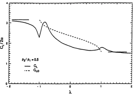
Using the airfoil boundary conditions, time varying vorticity on the blade can be found. A general, analytic solution for the vorticity was not given by Marble. He instead used computational methods to integrate his analytical equations which were based on satisfying the boundary conditions on the flat plate. This gave solutions for the lift and moment on the flat plate as a density jump convects along the airfoil. In figures 2.2 and 2.3 the lift and moment for a density change of _Pi - 0.5 are

plotted. The values for lift and moment excluding the effects of induction are plotted as dotted lines. The features of this problem will be described with reference to the lift coefficients. As the density jump approaches within about one half chord of the leading edge, the induced downwash generates a reduction of airfoil vorticity distribution, and consequently a lift reduction. As the discontinuity passes the leading edge, a strong upwash is produced, creating a situation resembling a sharp-edge gust. The subsequent rise in CL overshoots the value of CLo because of poor numerical spatial resolution. The moment coefficient, see figure 2.3, reflects these events in local loading. The response as the density jump passes off the trailing edge is relatively

CS 0--2 Figure 2.2: Lift -a = 0.5. Pl 0 d C4 -1 0 1 2

coefficient during passage of density discontinuity over the airfoil,

.2 .1 0 1 2

Figure 2.3: Moment coefficient during passage of density discontinuity over the airfoil,

Pa = 0.5.

Pl

mild because the value of vorticity is smaller in this region, consequently the near-field reflection is small.

2.2

Dimensional Analysis

Because scaling parameters are important and useful in engineering and scientific evaluations, a dimensional analysis is essential. Several methods for performing a dimensional analysis exist. Three methods for finding dimensionless parameters are by finding similarity solutions for the problem, using the Buckingham 7r theorem, or through an understanding of the physics of the problem. The physics involved in a density wake moving over a flat plate airfoil was used to non-dimensionalize basic equations.

The momentum equation is non-dimensionalized to find important parameters for this problem. An understanding of the physics of the flowfield outlined in 2.1 is essential to this analysis. In particular, the density parameter ( )~jj_ from Marble's linearized potential flow analysis should be a key parameter to this flowfield. Another important variable is the width of the strip. Remembering these parameters for the dimensional analysis gives

aj ₊ w = P2 - P1

-i = - ( )V( ) + viscous terms (2.10)

at c P2 + P1

where the new dimensionless variables are

( P (2.11) U t U= t _(2.13) ~ V V = - (2.14) C

S P (2.15) P1 + P2

This gives two important dimensionless parameters, (m) _c and (2).

\ P1 +P2

These two parameters are key variables in this computational experiment. An-other important parameter for this study is Re, the Reynolds number. The Reynolds number determines the boundary layer thickness and how turbulent the flow is. The three important dimensionless parameters for this problem are (v), p* = (P2

P ), and

Chapter 3

Computational Tools

Two separate computational tools were used to investigate this problem. Both tools solve the Navier-Stokes equations. An incompressible spectral element solver with pseudo-inviscid boundary conditions yielded inviscid solutions to the perturbation flow. A finite difference solver was then used to investigate the effects due to inter-action between the density wake and the blade surface boundary layer. These codes were chosen because they are higher order methods which give time accurate results with high spatial resolution.

3.1

Spectral Solver

A spectral Navier-Stokes solver written by Theodore Valkov [9] was used to ob-tain incompressible, pseudo-inviscid results. The Navier-Stokes equations are non-dimensionalized to freestream values giving:

Vi=0 (3.1)

=i -u ViV +1+ V( )V (3.2)

at Re

for laminar flow. The equations are made dimensionless by normalizing all distances by the stator blade chord cx, normalizing velocities by the axial freestream velocity

in units of (Ux). From this point the tildes no longer be used in this section, even thought he variables are still dimensionless. In the right hand side of equation 3.2, the first term represents the convection of the flow, the second term is the pressure, and the third is the effect of viscosity. These terms are solved for separately in the time stepping scheme.

3.1.1

Time Discretization

This spectral solver uses a fractional time splitting scheme. Starting from an initial flowfield, the scheme updates flow variables at each time increment in three fractional steps. The first step is the convective step which calculates the change in velocity from time t to time t + At due to convective effects only. The step uses a fourth order Runge-Kutta method to solve:

= - u. Vudt (3.3)

This velocity is next updated with the pressure step

-n+1 n1 -At n

u -+Vp"ldt (3.4)

using a backward Euler discretization. A pressure field pn+1 _{yields an updated velocity}

that satisfies continuity. The third and final step, the viscous step, updates the velocity to account for dissipation in the flowfield. An implicit Crank-Nicholson Scheme discretizes

n+ n+l t+At

u 1 u - (V(Re) Vu)dt (3.5)

while applying Dirichelet boundary conditions. This three step scheme has an error of O(At). It may become unstable if the time step is too large for the given grid resolution and Reynolds number.

Spectral element E is enlarged, showing collocation points and local coordinate system.

"II

Figure 3.1: Example of Spectral element gridding technique.

3.1.2

Spatial Discretization

The spatial discretization is performed by dividing the computational domain into spectral elements. Inside each spectral element(see figure 3.1),the flow variables are expanded in a series of local Lagrangian interpolants:

u

p j=0 k=o Pj,k

where uj,k and Pj,k are velocity and pressure values at the collocation point ()i,j in each element. These local interpolants are based on Chebyshev polynomials:

h,(s) = _n N _{( mE0} o 1 _T.(sn)Tm(S) (3.7)

The natural set of coordinates ((, q) local to each element is related to the physical

co-ordinate system (x, y) by an isoparametric tensor-product mapping. The coco-ordinates Y

4

of the collocation points in the local coordinate system are

((, r)j, = (cos N, cos (3.8)

During the discretization process, the periodic boundary conditions are implicitly implemented. To accomplish this the computational grid is generated so that nodes on the upper and lower boundaries have the same abscissas. A unique index, ()j,k, is then used for pairs of matching nodes on the periodic boundaries.

3.1.3

Boundary Conditions

As stated in the previous section, periodic boundary conditions are implemented on the upper and lower boundaries. The inlet boundary condition for the field is pre-scribed by a velocity profile. The outflow boundary condition is a simple extrapolation which assumes that the flow does not evolve in the streamwise direction aft of the outflow boundary.

Ou

S(x,

For the tests performed in this study, the flow is laminar. The spectral solver can compute turbulent flowfields at Re > 10,000 using a Baldwin-Lomax Turbulence model.

The original code written by Valkov assumed a constant density flow. Philippe Deregal modified the code to allow for incoming density wakes. Because of difficulty in altering incompressible code to allow for density changes, a slip boundary condition was imposed on the blade. This alleviates problems caused by the interaction between the density wake and the boundary layer on the blade because the boundary layer on the blade has been eliminated.

3.2

Finite Difference Solver

A finite difference Navier-Stokes solver written by Donald Hoying [2] was used to study the interaction between the density perturbation and the boundary layer on

the blade. Although the code was written for compressible flows, it was run at a low Mach number (M = 0.2) to simulate incompressible flow. Hoying's code was chosen because it uses a dispersion preserving scheme which is a higher order method that yields time accurate results with high spatial resolution.

3.2.1

Discretization

Instead of choosing discretization methods which produce highly accurate results, a method was chosen which has optimal dissipation and dispersion characteristics. This method, described by Tam and Webb [8], is referred to as a Dispersion Relation Preserving (DRP) scheme. The DRP scheme defines spatial and time discretization. Starting with a general description of a first derivative on a uniform grid gives:

(af\

1

M

- A =-N af (x + Ax) (3.10)

(ax)

In traditional finite difference schemes the coefficients at eliminate terms from the Tay-lor's series expansion of f. Instead an approximation to the derivative in equation 3.10 is considered in Fourier transform space. A Fourier transform of equation 3.10 gives

zaf _ x E aaela (3.11)

l=-N

From this a numerical approximation for aAx is defined as

M

aAx -_ dAx = -z alesalAx (3.12)

1=-N

where dAx represents the finite difference approximation of aAx. To obtain the best approximation of the derivative, the error function E should be minimized.

E a= oAx - &Ax|2d(aAx) (3.13)

0

V

I I I I

0 0.5 1 1.5 2 2.5 3

aAx

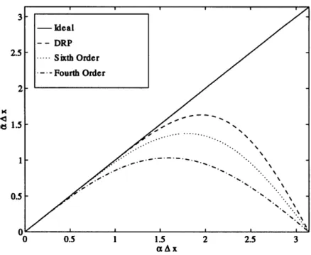
Figure 3.2: Comparison of DRP scheme with fourth and sixth order accurate scheme. The variable Oo represents the wave number range the error function is to be mini-mized over (-7r <

E

scheme. Since this scheme has seven points it can also be compared to a sixth or-der accurate scheme. From Figure 3.2 the DRP scheme has an improved range of accuracy compared to both the fourth and sixth order standard schemes. The DRP scheme also has improved accuracy in wave propagation speed.

The time discretization is formulated in a very similar way to the space derivatives, except a Laplace transform is taken instead of a Fourier transform. In construction of the higher order method, data from more than one previous time is used to update the current time step. In this formulation, values of time derivatives from previous time steps are used to update the current time step. These values come from the evaluation of space derivatives and any source terms. The time derivative can thus be written as

U(n+) - U(n) N dU (n -j)

Taking the Laplace transform of this equation yields

z(etwAt - 1) dU (3.15)

7_ - -W. _(3.15)

zAt Ej=0 Nbje3wAt dt

From this a numerical approximation to the ideal variable w can be defined as

z(ewas - 1)

At - wAt (3.16)

j=0 '3"

As with the spatial discretization, the numerical approximation DAt can be optimized with respect to wAt. The error function E is defined as

E =] {[( A[R(t - wAt)]2 + (1 - a)( t - wt)] 2}d(wAt) (3.17)

The variable a is used as a weighting factor between the wave propagation character-istics (real part) and the dissipation (imaginary part).

As with any high order method, the presence of high frequency waves in the solution is a concern. The DRP method is not subject to odd-even decoupling; it does capture unwanted high frequency waves. These waves are easily created at interfaces with solid surfaces and inlet/exit boundaries. The method used for damping is similar in construction to the method used to approximate the space derivatives. The artificial damping used takes the form

M U( n + l ) -_-i U"_i ) = o _{O E} E cU(n)_.i+j

j=-N

The variable Po is a constant used to adjust the amount of damping. The method cho-sen for this solver was to evaluate the fourth derivative of pressure at each point and use that value to scale Iuo. This method proved very effective in selecting and remov-ing unwanted high frequency waves from the numerical solution without providremov-ing excessive damping of the desired waves.

3.2.2

Gridding Methods

For this solver multiple overlapping grids are used. The flow can be thought of as containing two unique regions: flow about the blades and the flow in the upstream and downstream ducts. These regions have distinct geometries and different flow characteristics. Flow in the duct is governed almost exclusively by the Euler equa-tions. Since the grid is a simple rectangular shape, a simple rectangular(H) grid is used to simplify computation in this region. In fact the geometry is so simple, that the grid lines are able to coincide exactly with the coordinate directions.

Near the blade surfaces viscous forces become very important to appropriately describing the flowfield. Therefore in this region the grid should conform to the blade. In this region a circular(O) grid is used with closely packed spacing near the surface and greater spacing farther away from the blade. Grid orthogonality near the surface is also important. Because of the use of multiple grids a grid interpolation scheme is necessary to pass glow information from one grid to another. Interpolation is necessary because the O and H grids share no common boundaries.

Formulating boundary conditions at the inlet and exit of an unsteady flowfield is challenging. The goal is to allow the interior portion of the flow solver to 'feel' as if the boundaries are very far away. This is particularly difficult in unsteady flows. Simply placing the inlet and exit boundaries far apart is unacceptable due to the long time required for this large domain to react to any unsteady behavior. The linearized Euler equation, which is solved over the H grid, has four possible eigenmodes which specify the flow solution. Along with these eigenmodes are their associated eigenvalues which determine the direction information in the eigenmodes travel. The goal of non-reflecting boundary conditions is to allow all outgoing eigenmodes to leave without generating any incoming modes. This solver uses the approximate unsteady method as described by Giles [1].

Chapter 4

Inviscid Flow Response

To gain a basic understanding of the flow physics, the problem of a density gradient convecting over a blade row is first investigated by looking at this unsteady problem in an incompressible, inviscid flowfield. Knowledge of the basic flow physics will serve as a building block toward compressible and viscous flows. This section details the effects of a single density gradient convecting over a compressor blade row in an inviscid, incompressible flowfield.

4.1

Introduction

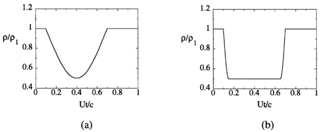
The effect of a convecting density distortion on an inviscid, incompressible blade row was investigated by running a series of computational experiments. The density dis-turbance used for this study is a planar disdis-turbance(normal to the blade row) which varies for freestream density (p1) to a peak density (P2) and back to freestream den-sity(see figure 1.1). Two forms of density variation are studied: a sinusoidal density variation and a flat top density change (see figure 4.1). The sinusoidal wake has a (1 - sin( Ut)) distribution, so there are no sharp changes in the density distribution of the wake. The 'flat top' also has this type of density change. The flat top changes density sinusoidally over a width of E C = 0.05 at the leading and trailing section of the wake.

1.2 , , , 1.2 1 1 P/P 0.8 -P/ 0.8 0.6 0.6 0.4 0.4 0 0.2 0.4 0.6 0.8 1 0 0.2 0.4 0.6 0.8 1 Ut/c Ut/c (a) (b)

Figure 4.1: Density variation over time for one density distortion. Sinusoidal density change(a) and flat top density change(b) go from free stream density(p₁ to peak density P2 and return to free stream pl.

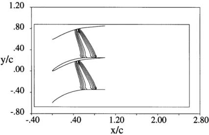
varied. These parameters include: blade geometry, magnitude of density change, and width of density distortion entering the passage. For these tests two blade shapes are studied(see figure 4.2). One blade, referred to as the EEE blade(see figure 4.2a), is highly loaded and has a fairly uniform pressure distribution. The other blade, referred to here as NACA4F(see figure 4.2b), has a lower loading with most of the pressure change occurring over the front half of the blade. All tests were run with flow at incidence to these blades.

Only one density wake convects through the passage for this investigation. Most tests were performed on the NACA4F blades; only four tests were run with the EEE blade row, all with sinusoidal density variations. The parameters for these tests are a density parameter p*, defined as (P2-P), and wake width (") where c, the chord length, non-dimensionalizes the width w of the wake. The tests for the EEE blade include

1. p* = - with - = 0.1

2. p* = with - = 0.1 and 0.2 3. p*= with - = 0.2

Various tests were run on the NACA4F blade. Table 4.1 show the test matrix for sinusoidal wakes encountering this blade shape. Flat top distortions were also run

_ ] p* 0.1 2 _3' 1 1 1 1 1 3' 6' 9' 6' 3 0.2 _3' 1 1_{9' 6} 0.4 2 1 1 1 1 1 3' 3' 9' 9' 6' 3 0.6 1₉

Table 4.1: Table of test matrix

(a) (b)

Figure 4.2: Blade geometries used for numerical experiments: EEE blade(a) with blade loading e _ 0.5 and NACA4F blade(b) with 0 r 0.31.

with the NACA4F blade row, all with the same density change and density gradient. Five widths for the flat portion of this distortion are examined. As a starting point, a width of zero is used which compares with sinusoidal tests. The other variations include widths of 0.2,0.6, 0.8, 1.3, and 1.6 chord lengths. Thus the factors affecting loading are not only the width and strength of the density wake, but also blade loading and the form of the density change.

Before continuing with results of the experiments, the general physics of the flow-field will be reviewed. For this explanation a wake with a density deficit will be considered. As the wake approaches the blade row, the density distortion interacts with the blade row pressure field because the density gradient is nearly normal to a pressure gradient. This interaction creates added vorticity in the flowfield (see sec-tion 1.2 for more detailed explanasec-tion). As the wake encounters the leading edge, a downwash is induced on the blade reducing the blade angle of attack. As the wake passes midchord, an upwash is induced on the blade which causes an increase in angle of attack. This translates into a decrease then an increase in lift. For a wake of higher density relative to free stream the opposite will occur. As the wake encounters the

blade row an upwash will be produced, followed by a downwash as the wake passes mid-chord on the blades. So for a wake with higher density, the lift will increase then decrease to freestream value as the wake leaves the blade row.

4.2

Evolution of Density Wake

The density disturbance is introduced at the inlet to the computational domain( = -0.35) and convects with freestream velocity U,. As the density disturbance encoun-ters the blade row it interacts with the blade pressure gradient, causing a local change in velocity which alters the shape of the density disturbance as it flows through the passage. As the density disturbance enters the blade passage it immediately reacts with the blade pressure gradient. This reaction, as described in section 1.2 results in lower density flow migrating toward the low pressure(suction) side of the blade and the higher density flow moving toward the high pressure side of the blade row. This causes a change in wake shape from a planar disturbance to a more irregular shaped distortion.

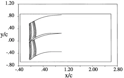
As the density wake convects through the passage, the disturbance density will migrate toward one side of the blade row. Upon encountering the blade row the density wake is cut by the blade row, just as a pressure wake would be [4]. An example with p* = -1 and ~ = 0.2 is shown in the plots of constant density in figures 4.3, 4.4, and 4.5. Time for these inviscid tests is normalized so that t = 0 corresponds to the wake encountering the leading edge of the blade row. Figure 4.3 shows the density wake at a time t = 0.15, corresponding to a midpassage position of the front of the wake of about - = 0.15 where -_{C C} = 0 is the leading edge of the blade. The blade row has cut the density wake, but the wake still has its planar shape. Figure 4.4 shows the wake at a later time t = 0.65 when the front of the wake at midpassage is at approximately 1 = 0.75. At this point the density distortion has been altered due to equilibrium conditions in the passage. The low density fluid in the wake is traveling toward the suction side of the blade, causing a larger concentration of low density fluid on the suction side. The wake has left the trailing edge of the

1.20 .80 .40

y/c

x/c

Figure 4.3: Plot of constant density showing position of the density disturbance at

t = 0.15 where the disturbance is defined by p* = -1 and _{3 c}- = 0.2.

blade row in figure 4.5. This corresponds to a time of t = 1.15 and a midpassage position of the front of the wake of ! = 1.28. The planar wake has distorted during its passage through the blade row. The wake has a thinner width at the pressure side of the blade row and a larger concentration of low density fluid at the suction side of the blade row.

A larger density gradient (smaller width for given p*) causes the wake to deform more quickly because a higher gradient creates more added vorticity, and thus greater circumferential velocity to transport the density toward one side of the blade. The low density disturbance changes from a planar wake to a blob of non-uniform density as it leaves the blade passage. A wake with a density increase reacts similarly except that the flow migrates toward the pressure side of the blade row and not the suction side. Thus as the density wake flows to the next blade row, its shape is no longer planar. The blade row pressure field changes the shape of density disturbances as they convect through the passage. The pressure difference in the passage has the effect of forcing the lower density fluid to the low pressure side of the passage to achieve equilibrium. This creates a concentrated mass of nonuniform density exiting the blade row. The form of a density wake entering a downstream blade row is thus greatly altered.

1.20 .80 .40

y/c

x/c

Figure 4.4: Plot of constant density showing position of d 0.65 where the disturbance is defined by p* = -1 ₃ and !L _C =

1.20

y/c

x/c

Figure 4.5: Plot of constant density showing position 1.15 where the disturbance is defined by p* = - and

2.80 ensity disturbance at t = 0.2. 2.80 disturbance at t = of density 1 c = 0.2. , . , , , , ,

1.20 .80 .40 i.. .00 " .40 .80 -.40 .40 1.20 2.00 2.80

x/c

Figure 4.6: Disturbance velocity vectors for sinusoidal density wake with p* = -1₃ and X _C = 0.2 at time t = 1.0

4.3

Induced Vorticity

A clear understanding of the changes in loading can be obtained by examining the

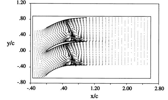
disturbance velocity field. For this purpose the density wake examined in figure 4.4 is studied. To conform with compressor nomenclature, the 'x' direction from the figure is referred to as the axial direction, and the 'y' direction is referred to as the circumferential direction. The test case in figure 4.4 involves convection of a sinusoidal wake convecting over the NACA4F blade row. The density wake has a strength p* = -1 and a width of X = 0.2. A density deficit causes a downwash as the wake encounters the blade and an upwash as the wake passes midchord. As the density distortion encounters the blade row, counterrotating vorticies are formed along the density distortion. These vorticies can be clearly seen by examining the disturbance velocity vectors, (see figure 4.6). In this figure the wake has convected t = 0.15, corresponding to the wake position as seen in figure 4.4. At the center

of the wake where the density peak negative circumferential velocity is formed(see figure 4.6). This translates into a force in the negative circumferential direction, causing a reduction in angle of attack and therefore a reduction in lift. As the velocity

perturbation travels to the back half of the blade, the negative circumferential velocity translates into an increase in blade angle of attack and thus an increase in lift. This varying force gives an unsteady moment on the blade. The unsteady moments for this study are calculated about midchord. The downward velocity created as the wake convects through the passage creates a counterclockwise moment as the wake convects over the first half of the blade and a clockwise moment as the wake travels over the back half of the blade. Therefore the time varying moment will increase then decrease to freestream value when the wake is at the midchord. The moment will decrease farther and then increase to freestream as the wake leaves the trailing edge. These disturbance flowfields also indicate how parametric changes affect blade loading. Changes in the wake parameters alter the added vorticity in the flowfield. The three parameters which define the wake are the distribution of the density change, the strength of the density wake(p*), and the width of the wake(c). Two wake shapes are examined, a sinusoidally varying density change and the flat top density change(figure 4.1). Two wakes with the same width and strength but different distri-butions will have very different effects on the flowfield. The flat top wake has a higher density gradient because the density change occurs over a much smaller length. A higher density gradient means that more vorticity is created, from the vorticity equa-tion

Dw 1

D = -- (Vp x Vp) _(4.1)

Dt p2

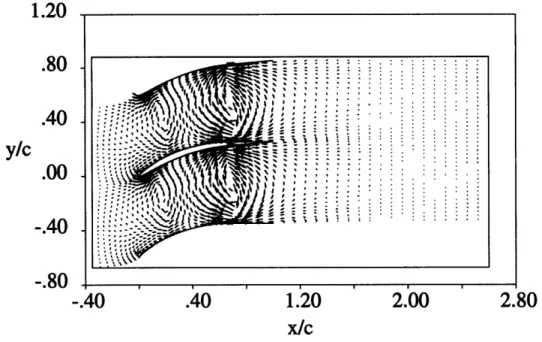
So a flat top has a higher density gradient and thus creates more added vorticity in the blade row. This is clearly illustrated in figures 4.7 and 4.8 where a sinusoidal and flat top wake have convected through the passage, creating added vorticity and thus a disturbance velocity field. Both wakes have a strength p* = 1 and a width - = 0.6. The wakes have traveled the same distance as those in figure 4.4, but are three times as wide. Because the density parameter is smaller in magnitude these disturbance fields are scaled to three times those of figure 4.6 to make the disturbance vectors more visible. Each wake creates counterrotating vorticies because the density first increases then decreases. The centers of these vorticies are farther apart for the flat

1.20

-- °

.80 , ,, .

-.40 _y/Cx/c .40 1.20 2.00 2.80

W _{= 0.6 at time t = 2.0.}

top wake. This changes the time scale between the two wake shapes. The flat top

wake loading changes faster because the center of the first flat top vortex has traveled farther than the sinusoidal wake vortex for the same convective time. The peak in loading will occur at the same time for the wakes because the wakes are of the same width.

The added vorticity in the passage is also dependent upon the strength of the wake. The magnitude of density change determines the magnitude of the vorticity. For a constant wake width an increase in the magnitude of the strength(p*) of the wake will increase the vorticity. Also a change in the sign of the strength(density deficit or increase) will change the orientation of the vorticies(see figures 4.6 and 4.7). The width of the wakes determines the distance between the centers of the counterrotating vorticies. Thus for larger wakes the vorticies will be farther apart and will not have as strong an influence on each other.

The density distortions are defined by their strength(p*), width(M), and density distribution. These parameters directly relate to the changes in vorticity. Any change which alters the local density gradient will alter the vorticity. This change then

1.20

.80

,

.40

-0.2/

x/c

at time t = 2.0

_.40.4

_{Pressure Distributions}

_Static

.80 ,

_-.

₄₀

_.40

_1.20

_2.00

_2.80

x/c

Figure 4.8: Disturbance velocity vectors for flat top wake with p = and = 0.6 at time t = 2.0.

translates into a change in the magnitudes of the time varying lift and moment. The change in vorticity also relates to a change in static pressure distribution on the blade. Static pressure changes can then be translated into changes in lift and moment.

4.4

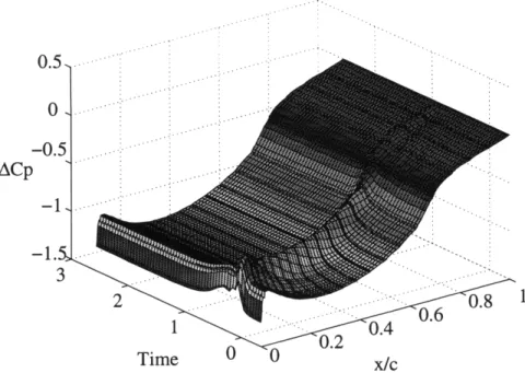
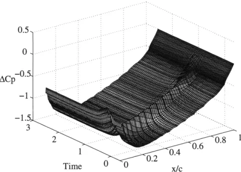
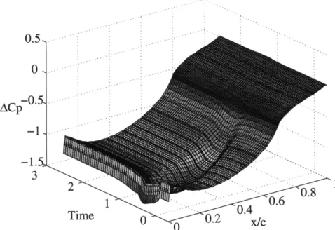
Static Pressure Distributions

The static pressure distribution across a blade row affects the unsteady loading caused by a convecting density wake. The effect of differences in pressure distribution across the blade row directly affects the changes in loading caused by a density wake. The two blades studied, the EEE blade and the NACA4F blade, have very different pressure distributions. Figures 4.9 and 4.10 show the difference in static pressure coefficient across the blades as a sinusoidal wake with p* = - and - = 0.2 convects through the passage. Both figures show the static pressure difference across the blade row, start-ing just aft of the leadstart-ing edge of the blades. The steady state pressure distribution is represented at time = -0.35, before the wake enters the passage. The EEE blade has an even pressure loading, but the NACA4F blade is forward loaded. The trailing