Ministère de l
’Enseignement Supérieur et de la Recherche Scientifique
Université de Batna 2
– Mostefa Ben Boulaïd
Faculté de Technologie
Département d
’Electronique
Thèse
Présentée pour l
’obtention du titre de :
Docteur LMD 3
èmeCycle en Electronique
Option : Hyperfréquence et traitement du signal
Sous le Thème :
Analysis by the full wave approach of patch resonators embedded in multilayered medium containing isotropic dielectrics, anisotropic substances and chiral materials
Présentée par :
Youssouf BENTRCIA
Devant le jury composé de
:
Mr. MAHAMDI Ramdane Prof. Université de Batna Président
Mr. FORTAKI Tarek Prof. Université de Batna Rapporteur
Mr. BENATIA Djamel Prof. Université de Batna Examinateur
Mr. CHAABI Abdelhafid Prof. Université Frères Mentouri Examinateur
Constantine
Mr. BEDRA Sami MCA Université de Khenchela Examinateur
This thesis presents a full wave analysis of microstrip patch embedded in a multilayered medium containing isotropic or anisotropic dielectrics and chiral substances. The analysis is based on the derivation of the dyadic Green’s function in the spectral domain. Then the electric field integral equation is formulated, and solved by the method of moments. The resonant frequency and the bandwidth of the antenna are computed by finding the complex roots of the determinant of the impedance matrix. Stationary phase theorem is used to compute the far-field and thus determining the antenna radiation pattern. A parametric study is achieved to investigate the influence of the patch dimensions and the substrate characteristics, including the effect of anisotropy, on the resonance and the radiation characteristics of the microstrip antenna. The mathematical details of the formulation are presented. The basic theory involved in the modeling of the electromagnetic field with chiral media is provided, and the different approaches proposed in the literature are mentioned. The influence of chirality on the resonant frequency, bandwidth and the far field is shown. Finally, an introduction into the modeling of the different feeding techniques and the effects of two feeding techniques on the antenna performance is presented.
Cette thèse présente une analyse rigoureuse d’un résonateur patch noyé dans un milieu multicouche qui contient des matériaux isotropes, ou anisotropes et des substances chiraux.
L’analyse est basée sur le calcul de la fonction dyadique de Green formulée dans le domaine
spectral. Ensuite, l’équation intégrale du champ électrique est formulée. La méthode des moments est utilisée pour résoudre l’équation intégrale. La fréquence de résonance et la bande passante sont calculées en cherchant les racines complexes du déterminant de la
matrice d’impédance. Le théorème de phase stationnaire est exploité afin de déterminer le
champ électrique lointain, ce qui permet la détermination du diagramme de rayonnement. Les effets des différents paramètres de la structure sur les caractéristiques de résonance et
rayonnement de l’antenne microbande, ont été analysés, notamment les dimensions du
patch et les caractéristiques de substrat en plus de l’effet de l’anisotropie. Les détails mathématiques de la modélisation ont été présentés. La théorie qui décrit l’interaction du champ électromagnétique avec les milieux chiraux, est présentée. En plus, les approches proposées dans la littérature pour modéliser ce genre des milieux, ont été mentionnées. L’influence de chiralité sur la fréquence de résonnance, la bande passante et le champ rayonné est présentée. Finalement, une introduction est présentée sur la modélisation des différentes méthodes d’excitation et l’influences de deux techniques sur la performance de
صخلم
ينبم سارد د ت ح رطلأا هذه ع بطلا ةددعتم لز ع ةد م ينب نمض ع بطملا يئا لا ساردل لم ش جذ من ينبلا حت نأ نكمي مك ، ف صم أ يم س دادعأ لكش ع با ثب فص ت نأ نكمي يئ يزي لا صئ صخ نأ ثيح نم دا م ع ن .لاريك ي م كتلا لد عملا ب تك ث ،ي يطلا ل جملا يف نيرغ لاد جارختسا ع ينبم ينبلا هذه سارد لذ دعب ،يئ بر كلا ل ح ل ي . لد عملا هذه لح لجلأ زعلا يرط يه يددع يرط ادختسا ت ضرع نينرلا ددرت صم زيممل بكرملا ر ذجلا د جيإ يرط نع م ب سح ت طنلا ر تسملا ر طلا يرظن ادختسا ت منيب . عن مملا ف ع هرثأ لما علا ف تخم سارد ت .يئا ل ب ص خلا ع عشلإا ططخم جارختسا يئ بر كلا ل حلا سحل لا ةد ملا صئ صخ لذك ع بطملا طيرشلا صئ صخ يف يس سأ لكشب لثمتت لما علا هذه ،يئا ل ي يظ لا صئ صخ سملا لز علا ل حلا لع ت فصت يتلا يس سلأا ئد بملا .عبتملا جذ من ل يض يرلا نا جلا ضرع ت مك . مدخت نم دا ملا عم يسيط نغم ر كلا نم ع نلا اذه ساردل حرت ملا تخملا جذ منلا ركذ ت مك ، ضرع ت لاريك ع ن دا ملا ملا نم ع نلا اذ ل ةزيمملا يص خلا رثأ نيبت لإ ف ضلإ ب يئا ل ي يظ لا صئ صخلا ع دا ت ،ريخلأا يف . اذك ، ع بطملا يئا لا يذغتل معتسملا ين تلا ف تخم جذمن نع مد م ء طعإ سارد ين تلا هذه نم نيع ن ريثأت . يئا لا هذه ءادأ عI would like thank my advisor Pr. Tarek Fortaki, for his guidance, advices and
support during the time required to prepare this thesis. I would like thank also
the friends, the colleagues and the people how have aided and encouraged me
to accomplish this work.
Introduction ………. 9
1. Computational electromagnetics 1.1. Introduction ………. 14
1.2. Analytical models ……….... 1.2.1. Transmission line model .……… 1.2.2. Cavity model ....……….. 18
1.2.3. Multiport connection method ……… 19
1.3. Numerical methods ……….. 1.3.1. Differential equation methods ……… a. Finite element method ……….. b. Finite difference methods ………. 8
c. Transmission line matrix method ………. 1.3.2. Integral equation methods ……….. 6
a. Finite integration technique ………. 6
b. Partial element equivalent circuit method ………. 8
c. Method of moments ……….. 39
1.4. Green’s fun tions ……….. 1.5. Conclusion ……….. 2. Full wave analysis of microstrip patch embedded in a multilayered medium containing isotropic or anisotropic materials 2.1. Introduction ……… 8
2.2. Theory ………. 50
2.2.1. Derivation of dyadic Green’s function ……… 51
2.2.2. Formulation of integral equation ……….. 7
2.2.3. Solving the integral equation ……… 7
2.3. Results and discussions ……….. 9
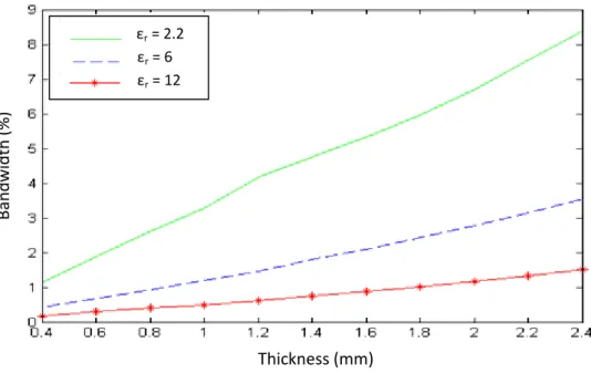
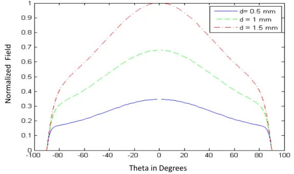
2.3.1. Effect of dielectric parameters ……… 9
a. Effect of thickness ……… 9
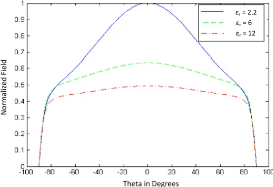
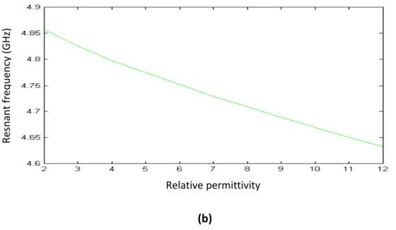
b. Effect of permittivity ……….. 62
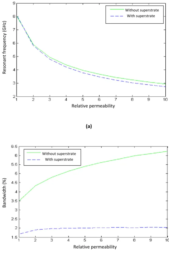
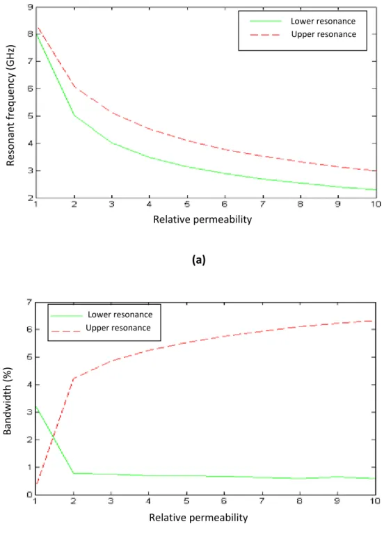
c. Effect of permeability ………. 65
d. Effect of anisotropy ………. 8
2.3.2. Effect of patch dimensions ……… 72
2.4. Conclusion ……….. 78
3. Full wave analysis of microstrip patch embedded in a multilayered medium containing chiral materials 3.1. Introduction ……… 81
3.3. Results and dis ussions ……… 89
3.4. Conclusion ……… 93
4. Feeding techniques 4.1. Introduction ………. 96
4.2. Theor ……….. 98
4.2.1. Microstrip line feed ……… 98
4.2.2. Coaxial probe feed ………. 101
4.2.3. Proximity coupling feed ………..……… 104
4.2.4. Aperture coupling feed ………..………. 106
4.3. Results and discussions ……… 111
4.3.1. Mi rostrip line feed ……… 111
4.3.2. Coa ial pro e feed ……….. 5
4.4. Conclusion ……….. 118
Con lusion ………. 120
References ………. 123
9
The first microstrip patch antennas have been fabricated on single layer isotropic substrates. The emerging trend toward multilayered configurations was imposed by many practical needs. For instance, in wireless applications, cover layers have been used for protection against environmental effects. Also in microwave circuit applications where microstrip antennas are integrated with feed networks and active devices, multilayered substrates are used extensively [1] – [3]. The inherent narrow bandwidth of microstrip antennas requires modeling methods capable of accurately predicting the resonant frequency and examining the possible effects of different parameters on the antenna performance. The available methods for such task are based on full wave approach and they are implemented using numerical methods. These methods account rigorously for all radiation, coupling and loss mechanisms. Furthermore, they are powerful tools for modeling arbitrarily shaped radiating elements, arrays and different feeding techniques [4], [5].
Early substrates used for microstrip antenna technology, were isotropic. However, it was proven that even the dielectrics considered isotropic, posses some amount of anisotropy. In addition to the fact that, some artificial anisotropic materials are intentionally used to achieve certain operational characteristics. Therefore, an accurate characterization of the
effect of anisotropy on the antenna performance is needed [6] – [8]. Chiral materials gained
a significant interest in electromagnetics community, where a great amount of research has been accomplished on the theory of electromagnetic wave propagation in chiral media. The research on chiral media, which is a bi-isotropic media, has been accomplished in the course
10
for the analysis of microstrip patch embedded in a multilayered medium containing isotropic, anisotropic and chiral materials.
The thesis is organized in the following manner:
The first chapter presents an overview on two broad categories of methods developed for modeling RF and microwave devices. These categories are, simplified or reduced analysis based methods, and full wave or rigorous analysis based methods. Reduced-analysis approaches are based on the use of simple physical models, where simplicity and physical insight are granted at the expense of accuracy. These methods are generally, of a limited scope. In this chapter, transmission line, cavity and multiport connection models are described and their features are presented. Then, a comparison is made between these models in terms of different criteria. Full wave approaches are based on the use of numerical methods; these methods sacrifice simplicity and physical insight at the expense of accuracy. These methods are the core algorithms of almost all CAD commercial microwave packages. The Numerical methods presented in this chapter, are classified according to the kind of equations usually, these methods are applied to. Thus, we will have two categories:
Differential equation methods and integral equation methods, finite element method, finite difference and transmission line matrix methods are treated under differential equation methods. Whereas, the method of moments, the finite integration technique and partial element equivalent circuit methods, are treated under integral equation methods. At the end of this chapter, the most popular methods are compared in terms of their performance and features. Since the method of moments requires the formulation of the appropriate
11
methods used to derive Green’s functions.
In chapter 2, an efficient algorithm based on the use of spectral dyadic Green’s function and
the method moments, is provided. This model is used to characterize a microstrip patch embedded in a multilayered medium, where the dielectric can be isotropic or anisotropic. The resonant frequency and the bandwidth are computed by seeking the complex roots of the determinant of the impedance matrix. The radiated field is calculated using the stationary phase theorem. The mathematical features of the present formulation, makes it an efficient tool for analyzing stratified media. The use of the concept of transfer matrix to represent the layered medium is of a great importance for two main reasons; it allows the
formulation of the Green’s function easily, furthermore, the characteristics of each layer are
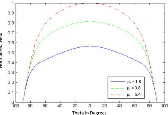
easily included. A parametric study on the influence of the patch dimensions, the permittivity, permeability and the thickness of the substrate, is provided. Also the effect of electric and magnetic anisotropy is investigated.
Chapter 3 provides a survey on the theoretical models proposed for the study of electromagnetic wave propagation in a chiral media, and the refection and scattering from achiral-chiral interface. A comprehensive formulation describing the process yielding the derivation of dyadic Green’s function in the Fourier transform domain. The process starts from the constitutive relations of a chiral media, and proceeds until the transverse components of the electric and magnetic fields are written, in spectral domain, in terms of longitudinal components of right- and left-circularly polarized waves. Enforcing boundary
conditions yields the derivation of the corresponding Green’s function. The effect of chirality
12
formulation of popular feeding techniques, namely microstrip line, coaxial probe, proximity coupling and aperture coupling feeding techniques. The influence of the parameters of two feeding techniques is presented. Finally, summary and discussion results are listed in the conclusion.
Chapter 1:
Computational
Electromagnetics
14
1.1. Introduction
Electromagnetic analysis treats the interaction of the electromagnetic fields with objects and the surrounding environment. The analysis approaches can be divided into two broad categories, reduced or simplified analysis and full wave analysis. In the reduced-analysis, some approximations are made in the description of the problem; these simplifying assumptions allow the use of simple physical models where the analysis results are close to those of the original problem. Simplified analysis usually employs analytical methods, and these methods maintain simplicity at the expense of accuracy or versatility. On the other hand, full wave analysis involves the use of numerical methods. These methods maintain rigor and accuracy at the expense of computational simplicity.
The applied methods in the modeling of the electromagnetic fields and devices can be classified as [13], [14]:
Analytical methods: where closed-form solutions are obtained through the use of analytical formulas.
Semi-analytical methods: which provide explicit solutions requiring final numerical evaluation (such as complicated integrals, i fi ite se ies …)
Numerical methods: these methods transform the integral or differential equations of Maxwell (or an equation derived from them), into an approximate discrete formulation (matrix equation) solved directly (by matrix inversion) or iteratively.
We will start by describing the popular analytical models as applied for microstrip antenna structures. These models can be classified into three main models: transmission line model, cavity model and multiport network model.
15
1.2. Analytical models
1.2.1. Transmission line model
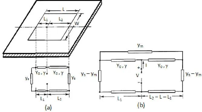
The transmission line model is the first technique employed to analyze a rectangular microstrip antenna by Munson in 1974 [14]. In this model, the microstrip patch antenna is assimilated to a section of a transmission line of length L where its characteristic impedance and the propagation constant are determined by the patch size and the substrate parameters. The edges of the patch are classified into radiating and non-radiating edges such as the radiating edges are associated with slow (uniform) field variations along their lengths, whereas non-radiating edges have an integral multiple of half-wave length variations along each edge which results in almost complete cancellation of the radiated power at these edges [14]. Usually, the radiating edges are considered as two narrow apertures (slots), each of width W, height d (representing the substrate thickness) separated by a distance L Fig.1. Each of the two slots is represented by a parallel equivalent admittance
Y with a conductance G and a susceptance B Fig.2.
16
Fig. 2 (a) Rectangular patch, (b) Transmission line equivalent
Where Yc is the characteristic admittance (it is related to the characteristic impedance Zc by
Yc = 1/Zc). The conductance G is associated with the radiated power, and the susceptance B
is related to the stored energy in the fringing field near the edge [5], [14]. The resonant frequency is function of the ratio L/d. The determination of the resonant frequency requires the computation of the effective length of the patch which is a result of the fringing, and the effective dielectric constant which accounts for the Quasi-TEM nature of the wave in the microstrip antenna structure. This model is conceptually simple, however, it is very approximate and the model is applicable only for a rectangular patch, besides, the effects of substrate on radiation and input impedance, are not considered.
Further improvement is achieved on this model by including mutual coupling between the radiating edges through a mutual admittance Ym connected between the two ends of the
transmission line [15], as depicted in Fig. 3. In Fig. 3, y0 is the characteristic admittance, ys is
the shunt load admittance and ϒ is the complex propagation constant having the form ϒ = α
17
Fig. 3 Transmission line equivalent circuit (a) simple model (b) including mutual coupling
The improved transmission line model can be applied on rectangular and square microstrip patches only. Furthermore, only microstrip and coaxial feeds are supported. Proximity- coupled and aperture-coupled fed microstrip antennas cannot be analyzed.
More elaborate model called the generalized transmission line model GTLM [16]-[18] has been proposed. In this model, transmission line sections, which may be non-uniform, on
either sides of the current source (which ep ese ts the feed), a e o e ted i to π-network
equivalent circuit. This equivalent circuit is then simplified using the star-delta and delta-star transformations to obtain the voltage across the current source [19]. GTLM can be applied to any separable geometry of the microstrip antenna including rectangular, circular and annular ring patches, with linear or circular polarization. However, the application GTLM to an arbitrary patch shape is not possible. Also, some of the feeding techniques such as Proximity- coupled and aperture-coupled microstrip feeds cannot be modeled.
18
1.2.2. Cavity model
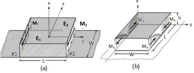
Microstrip antennas are narrow-band resonant antennas, so they resemble dielectric-loaded cavities. But unlike cavities, microstrip patch antennas are radiating elements; therefore they must be treated as lossy cavities. Cavity model was advanced by Lo et al [20]-[22], where the microstrip antenna is modeled as a cavity bounded by electric walls on the top and the bottom, and magnetic walls along the periphery. We should point out that, in this model, the substrate is assumed truncated and it does not extend beyond the edges of the patch. The patch antenna is represented by four slots, only two (the radiating slots) account for most of the radiation, the fields radiated by the two (non-radiating slots) cancel along the principle planes as shown in Fig. 4.
Fig. 4 Electric field in (a) radiating slots and (b) non-radiating slots of microstrip patch
Various types of losses (such as dielectric, conductor and radiation loss) are characterized in
the cavity model by an effective tangent loss δeff which is related to the quality factor Q by
δeff = 1/Q. The resonant frequency of the antenna is defined to be the resonant frequency of
the cavity for a given mode. Different patch shapes with linear or circular polarization and even stacked patches antennas have been treated by the cavity model. Also, the mutual
M1
E
1M
219
coupling between the apertures is included implicitly, however, the cavity model does not estimate the ratio of aperture fields correctly in microstrip antennas with more than one aperture therefore cavity model is not suitable for array applications [14].
The cavity model also has been generalized to analyze non-separable geometries [23], [24], where Green s functions have been used. In this model, the analysis of a given geometry proceeds as the following:
First, the given geometry is converted into an equivalent geometry with magnetic walls at the peripheries.
Then, the geometry with the magnetic walls is segmented into regular geometries for which Eigen-functions are available.
The planar circuit approach [25] is applied to determine the electric fields under the patch.
Next, the quality factor of the patch cavity is calculated using the procedure given in the cavity model.
Finally, the input impedance can be obtained from the ratio of the voltage and the current at the feed point.
This approach has been used to analyze a rectangular ring, cross-shaped and H-shaped patches.
1.2.3. Multiport Connection Method
Multiport connection method (MNM) model [26] can be considered an extension of the cavity model in which the impedance boundary condition at the periphery is enforced explicitly. This model takes into account the mutual coupling between various edges. The
20
MNM use the planar circuit approach [25], where the field in the interior region is modeled as a multiport planar circuit with ports located all along the periphery. The field in the exterior region, which includes the fringing fields, the radiation fields and the surface wave fields, are represented by load admittances. Unlike transmission line model, all the edges, radiating and non-radiating are represented as load admittances in the MNM. Table 1 provides a comparison between the different analytical models that have been presented in the literature for the analysis of microstrip patch antennas.
1.3. Numerical methods
Finding a solution for practical problems is a complex task. It requires simplifying assumptions and/or numerical approximations [27]. Analytical models, as we have seen, are based on analytical formulas which are exact, however, the made simplifying assumptions make them applicable to only a limited set of problems [28]. In the other hand, the approaches relaying on numerical methods, although their results are also approximate, but they generally offer results with good accuracy. Besides, they are applicable on wide range of problems which makes them the preferred choice for solving most of engineering problems. Eventually, even numerical methods based approaches make some simplifying assu ptio s su h as i fi ite diele t i a d g ou d pla e, ze o thi k ess st ips o pat hes… etc [27]. Solving electromagnetic field problems is known as computational electromagnetics CEM [27], or also numerical electromagnetics [13]. Full-wave analysis uses CEM methods as powerful tools to account rigorously for electromagnetic waves propagation in the structure under study.
21
Table 1 comparison of various analytical models [14].
Application Model Transmission line model GTLM Lossy trans. line Cavity model Generalized cavity.model MNM Patch shapes Rectangular only Separable geometries Arbitrary shapes Regular shapes Separable geometries Separable geometries Substrate thickness
Thin Thin Thin Thick Thin Thin
Feed type used Microstrip edge feed, probe feed Microstrip edge feed, probe feed Possibly all types Microstrip edge, probe and aperture feed Microstrip edge feed, probe feed Microstrip edge, probe feed and proximity coupling Circular polarization
No Yes No Yes Yes Yes
Stacked patches No No Yes Yes No No Mutual coupling between edges Explicitly included Explicitly included implicitly included implicitly included implicitly included Explicitly included Application to arrays
Yes Yes No No No Yes
The purpose of all numerical methods used in electromagnetics is to find approximate solutions to Maxwell s equations (or of equations derived from them) that satisfy boundary conditions [13]. That is why such kind of problems is referred to as boundary value problems [29], [30]. Almost all numerical methods in electromagnetics share the idea of discretizing some unknown electromagnetic property, that is , the unknown function (the solution) is expanded in terms of expansion functions with unknown coefficients [13], [27]. Nevertheless, numerical techniques have differences in their mathematical foundation which makes one technique more suitable for a specific class of problems compared to the other [28].
22
The classification of computational electromagnetics techniques can be made according to different criteria such as:
The quantity being discretized or solution variable (circuit or field variables) [27], [28] Domain of the solution (space and time or frequency)
Number of dimensions (1D, 2D, 2.5D, 3D) [13], [27].
The form of the equation(s) being treated by the method (differential or integral form) [31].
We note that, in general, the above classifications are not rigid, that is, labeling a method to as a time domain method does not mean that it cannot be applied in frequency domain, but rather it means that the method is usually applied in time domain. For instance, the methods usually applied in time domain include finite difference time domain (FDTD) and Transmission line matrix (TLM), where the methods usually applied in frequency domain include Finite element method (FEM) and the method of moments (MoM).
In this thesis, the numerical methods applied for the electromagnetic field problems, are classified on the basis of the form of the equations usually treated by these methods, and hence, they will be classified into differential equation methods (usually applied on partial differential equation or PDE), and integral equation (IE) methods, as shown in Fig. 5.
23
Fig. 5 Differential equation and Integral equation CEM methods
For a given application, some methods are more suitable than the others. For example [28]:
Electrical interconnect packaging (EIP) analysis (PEEC, MoM)
Printed circuit board (PCB) simulations (mixed circuit and EM problems) (PEEC) Coupling mechanism characterization (MoM, PEEC)
Electromagnetic field strength and pattern characterization (MoM) Antenna design (MoM)
Scattering problems (FEM, FDM)
The differences between the methods illustrated in Fig. 5, arise in two main points [28]:
Discretization of the structure: For the differential formulation, the complete structure including the air needs to be discretized. Whereas, in integral formulation, only the materials need to be discretized.
Solution variables: Differential equation based techniques deliver the solution in field variables i.e. electric and magnetic field. Post-processing of the field
24
variables is needed to obtain the currents and the voltages of the structure. For the integral equation based techniques, the solution is expressed in terms of circuit variables, i.e. currents and voltages. To convert the system current and voltages to EM field components, post-processing is needed.
In the following section, the concept and the main features of each of the methods illustrated in Fig. 5 will be presented.
1.3.1. Differential equation methods
a- Finite Element Method (FEM)
The laws of physics for space- and time-dependent problems are usually expressed in terms of partial differential equations (PDEs). For the majority of geometries and problems, these PDEs cannot be solved analytically. Instead, they are solved approximately, typically using different types of discretization [32]. Finite element method (FEM) is used to convert the PDEs describing a boundary value problem into a system of equations (matrix equation). FEM is powerful technique for handling problems involving complex geometries and heterogeneous media, and it is applicable in both time and frequency domain [28]. The procedure of FEM analysis can be summarized as the following [33]:
Discretizing the solution domain into a finite number of sub-domains or elements. Deriving the governing equations (elemental equation) for a typical element. Assembling all the elements in the solution domain to form matrix equation. Solving the system of the obtained equations.
The first step consists of subdividing the domain of the problem into smaller parts called finite elements, this process is called meshing. The shape of these elements depends on the
25
domain of the given problem. The advantages of the subdivision of the whole domain into smaller parts are [34]:
Accurate representation of complex geometry Inclusion of dissimilar material properties Easy representation of the total solution Capture of local effects
The element equations derived in the second step, are simple equations that locally approximate the original complex equation to be studied. Next, a global system of equations is generated from the element equations through a transformation of coordinates from the sub-domain local nodes to the domain global nodes. After that, the system of equations is solved by a direct or iterative method. Post-processing provides an estimate of the error in terms of the quantity of interest. When the error is larger than the acceptable value, the discretization level (i.e. meshing) has to be changed manually or by an automated adaptive process (adaptive meshing).
Generally, three approaches are being used when formulating an FEM problem [35]:
Direct approach Variational approach Weighted residual method
Direct approach:
This approach was applied initially in structural analysis, and it is theeasiest to understand because it involves the application of the concept of FEM it its simplest form. This approach consists of two steps: first, the system under consideration is replaced by an equivalent idealized system consisting of individual elements. These elements
26
are assumed to be connected to each other at specified points called nodes. When the elements are defined, the direct physical reasoning can be used to establish the element equations in terms of pertinent variables. In the second step, the individual element equations are combined to form the equations for the complete system, and then the system of equations is solved for the unknown nodal variables. This approach can be used only for simple problems.
Variational approach:
this approach relies on some variational principle such as theprinciple of minimizing the energy of a functional, where the energy can be obtained by integrating the (unknown) fields over the structure volume [36]. The variational approach is widely used whenever classical variational statement is available for the given problem. Such statement may not be available for some physical problems such as nonlinear problems.
Weighted residual methods:
It is a generic class that is developed to obtainapproximate solution to differential equations of the form:
ℒ 𝜙 + = In the domain D (1)
Where, 𝜙 is an unknown function (a dependent variable) of the variable x such as x ϵ D
Is a known function, and ℒ is a differential operator involving spatial derivatives of 𝜙
Weighted residual method involves two main steps. In the first step, an approximate
solution 𝜓 which satisfies the boundary conditions is assumed. The approximate solution
is expressed in terms of a sum that consists of (chosen) trial functions multiplied by unknown fitting coefficients. This approximate solution is substituted in the differential equation.
27
producing an error which measures the difference between the exact and the approximate solution, this error is called a residual R defined as
ℒ 𝜓 + = 𝑅 (2) The residual is then made to vanish in some average sense over the entire solution domain to produce a system of algebraic equations. Mathematically, this is accomplished by multiplying eq. (2) by weighting functions w(x) and integrating over the domain D to obtain
[ℒ 𝜓 + ] = 𝑅 (3)
Then, the weighted residual integral is forced to vanish over the solution domain, that is
𝑅 = (4) The second step is to solve the resulting system of equations to find the sought approximate solution by defining the fitting coefficients. Galerkin procedure, in which trial functions are equal to weighting functions, is among the weighted residual methods. FEM in general, has the following features:
Meshing of the entire domain is required (object + background) Great flexibility in modeling complicated and irregular geometries.
Good handling of inhomogeneous media, 2-D and 3-D linear and nonlinear problems Solution domain has to be terminated by numerical absorbing boundaries ABC or
perfectly matched layers PML. Widely used in frequency domain FEM produces large sparse matrices
28
b- Finite Difference Methods (FDM)
Finite difference methods (FDMs) are numerical methods for solving differential equations by approximating them with difference equations. The domain is partitioned in space and time (Fig. 6) and an approximation of the solution is computed at space and time points [37]. The error between the numerical solution and the exact solution is produced when going from differential operator to difference operator, and this error is called discretization or truncation error [37]. The main concept behind any finite difference scheme is related to the definition of the derivative of a smooth function in the neighborhood of a point x ϵ R:
′ = lim
ℎ→ 𝑥+ℎ − 𝑥ℎ ≅ 𝑥+ℎ − 𝑥ℎ for sufficiently small h. near the point of
interest (i.e. point x), ′ can be approximated by Taylor series.
Fig. 6 Discretization of the domain in space and time [38]
For the 1st derivative, we can distinguish forward-, backward- and central- difference approximations such as:
29 Forward difference: 𝜕𝜕 ≅ + , − , ∆ , 𝜕 𝜕 ≅ , + − , ∆ Backward difference: 𝜕𝜕 ≅ , − − , ∆ , 𝜕 𝜕 ≅ , − , − ∆ Central difference: 𝜕𝜕 ≅ + , − − , ∆ , 𝜕 𝜕 ≅ , + − , − ∆
For the second derivative, we have: 𝜕
𝜕 ≅
, + − , + , −
∆
Finite Difference Time Domain (FDTD)
Finite difference time domain (FDTD) belongs to finite difference methods. The first FDTD algorithm was established by Yee in 1966. FDTD is a numerical technique for finding approximate solutions for the associated system of differential equations, where time- and space- derivatives are approximated using finite difference expressions [36]. This method is widely used within electromagnetic modeling, mainly, due to its simplicity, where Maxwell s equations (in differential form), are discretized using central difference approximations to the space and time partial derivatives [31], [39]. In FDTD, the whole domain must be divided (discretized) into volume elements (cells), often, these elements are cubes (called voxels) [27]. For these elements, Maxwell s equations are approximated by finite difference equations. The volume elements sizes are determined by considering two main factors [36]:
Frequency: the cell size should not exceed λ/10, where λ corresponds to the maximum frequency in the excitation
Structure: the cell size must allow discretization of thin structures. The time step is limited by courant s condition [33]:
∆ ≤
30
The three-dimensional space of the problem is truncated by absorbing boundaries. The most popular absorbing boundary is the perfectly matched layer (PML) [31]. The unknown function to be computed for FDTD method is field variables i.e. electric and magnetic fields which are alternatively calculated at every half time step and at all locations of the discretized domain [33]. When Maxwell s equations are examined, it can be seen that the change in the E-field in time (the time derivative) is dependent in the H-field across space (the curl). This is the basic idea behind FDTD time-stepping relation that is, at any point in space, the updated value of the field in time is dependent on the stored value of the E-field and the numerical curl of the local distribution of the H-E-field in space. The H-E-field is time-stepped in a similar manner. At any point in space, the updated value of the H-field in time is dependent on the stored value of the H-field and the numerical curl of the local distribution of the E-field in space. This process known as loop-frog procedure, its algorithm is illustrated in Fig. 7 [31].
The FDTD method has the following advantages:
Simple implementation and easy to understand. No matrix inversion involved.
Easy modeling of complex material configuration
Since FDTD is a time domain technique, the response of the system over a wide frequency range can be obtained with a single simulation.
FDTD calculate the electric and magnetic fields everywhere in the computational domain as they evolve in time, which provides animated displays of the electromagnetic field movement through the model.
31
FDTD computes the electric and magnetic fields directly which is more convenient to EMC/EMI modeling.
A wide variety of linear and nonlinear dielectric and magnetic materials can be naturally and easily modeled.
Ability to perform both transient and steady state analysis. However, FDTD have some weaknesses such as:
Since the entire domain have to be discretized and the resulting elements must be sufficiently fine to resolve both the smallest wavelengths and the smallest geometrical feature of the model which results a large computational domain resulting a long simulation time.
The need of absorbing boundaries ABC (PML) to truncate unbounded problem domain
Difficulties with curve structures.
Finite Difference Frequency Domain (FDFD)
Finite Difference Frequency domain (FDFD) method is conceptually a simple method to solve time-dependent differential equations for steady state solutions. FDFD method transforms Maxwell s equations (or other PDE for fields and source), into a matrix equation of the form
A x = b where A is a matrix derived from the wave equation operator, the column vector operator x contains (the unknown) field components and the column vector b describes the source.
32
Fig. 7 Leap-frog algorithm
FDFD and FDTD share many common features. Beside the fact that FDFD is implemented in frequency domain, they are different in some points:
There no time step to be computed in FDFD
33
c-
Transmission Line Matrix (TLM) method
Transmission line matrix (TLM) is a space and time discretization method for the computation of the electromagnetic fields. TLM is based on Huygens principle Fig. 8 in which Huygens states that: All points on a wave front serve as point sources of spherical secondary wavelets. After a time t the new position of the wave front will be the surface of tangency to these secondary wavelets . This principle can be explained as the following:
At time 0 the central point scatters a wave. At time t1 all the points in the wave front are
acting as point sources, and the wave front at any time later, is the wave front from these secondary point sources.
34
Johns [40] modeled Huygens principle by sampling time and the space and representing it with a mesh of passive transmission line components. He modeled the wave propagation as voltage and current travelling in this mesh. The relationship between time sample Δt and
space sample Δl is given by: ∆ = ∆ where c is the free space light speed.
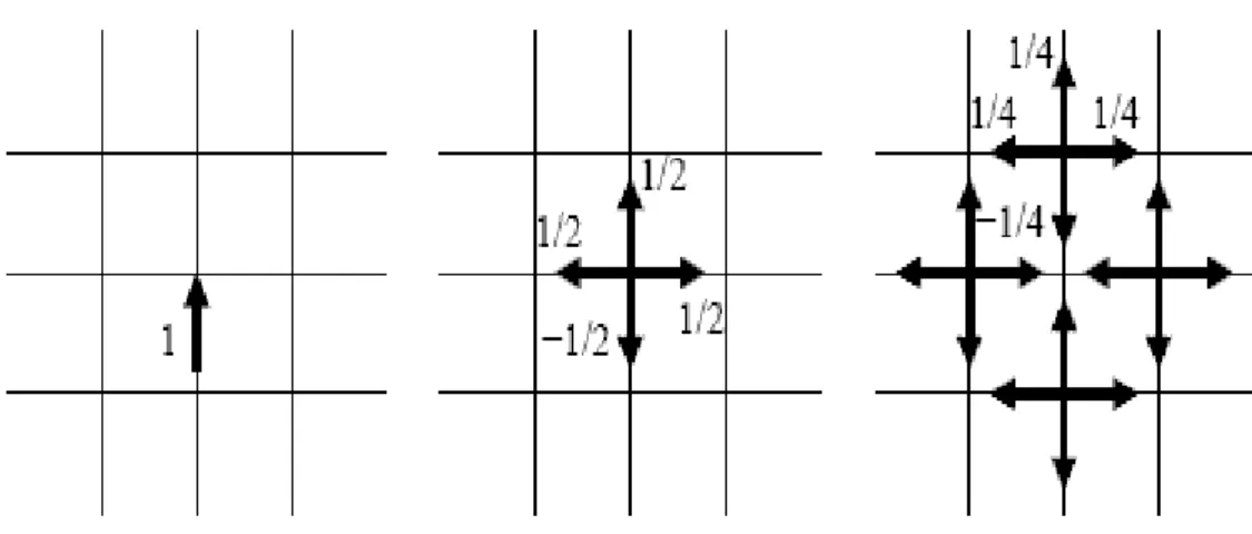
To understand the concept of TLM method, let us consider the TLM grid illustrated in Fig. 9. Assuming that at a time zero, an impulse is incident to the middle node, this node will scatter the wave to its 4 neighboring nodes. The scattered wave reaches these nodes at the
instant Δt. Now these four nodes will scatter waves to their neighboring nodes at time equal
to 2Δt. At each time step, each node receives an incident wave from the adjacent nodes and scatters it to the other adjacent nodes. By repeating the above process for each node, the wave distribution in the medium can be calculated. The choice of two- or three-dimensional TLM modeling depends on the complexity of the problem under study. In two-dimensional TLM model represented in Fig. 9, each node is surrounded by 4 nodes (Fig. 10), while in three dimensional TLM model (Fig. 11); each node is surrounded by 6 nodes (Fig. 12).
35
TLM method uses the concept of scattering matrix where (for 2D TLM model) the voltages
Vns representing the scattering waves, are related to the voltages Vni representing the
incident waves by [ 𝑉 𝑉 𝑉 𝑉 ] 𝐾+ 𝑆 = [ − − − − ] [ 𝑉 𝑉 𝑉 𝑉 ] 𝐾 (5) Where
S, I: Scattered and Incident waves respectively
K, K+1: arbitrary consecutive time steps
Based on the above equation, if the magnitude of the wave (voltage in the TLM modeling) is known at any instant KΔt, then the magnitude of the wave could be found at the instant
(K+1) Δt. By repeating this for each time step, wave propagation could be modeled. Similarly,
for three-dimensional TLM model, the eq. (5) could be rewritten as:
[ 𝑉 𝑉 𝑉 𝑉 𝑉 𝑉 ]𝐾+ 𝑆 = [ − − − − − − ][ 𝑉 𝑉 𝑉 𝑉 𝑉 𝑉 ]𝐾 (6)
TLM method can model homogeneous and non-homogeneous, lossless and lossy structures, each one requires different mesh model. TLM and FDTD are considered the most powerful time domain methods.
36
1.3.2.
Integral equation methods
a- Finite integration technique (FIT)
Finite integration technique (FIT) proposed in 1977 by Thomas Weiland, is a discretization method which is similar to FDTD method, however, FIT discretizes Maxwell s equations in their integral form. Maxwell s equations are transformed into a system of linear equations. This method is flexible in geometrical modeling and it handles curved boundaries and complex shapes with more accuracy. To explain the concept of the FIT, we consider Maxwell s equations for a linear and lossy medium [41]:
𝜕
𝜕 , 𝐴 = , − 𝜎 , 𝐴 (7)
𝜕
𝜕 𝜇 , 𝐴∗ = − , − 𝜎∗ , 𝐴∗ (8)
Where , and , represent the electric and magnetic fields respectively, and the
media parameters are described by the permittivity , the permeability 𝜇 , and the
electric and magnetic conductivity 𝜎 and 𝜎∗ . Equations (7) and (8) are approximated
by the finite difference equations:
𝐸ℎ𝑛+ − 𝐸ℎ𝑛
∆ 𝐴 = ℎ+ . − ℎ+ 𝜎 𝐴 (9)
ℎ𝑛+ .5− 𝐸ℎ𝑛− .5
∆ 𝜇 𝐴∗ = − ℎ − ℎ+ . 𝜎∗ 𝐴∗ (10)
Where Δt is the time step, ℎ and ℎ+ . are dielectric and magnetic field vector
approximated at time points nΔt and (n+0.5)Δt fo = , ,…
Then, FIT proceeds in a similar manner as FDTD. Both methods share advantages such as simple implementation and efficient parallel computing. They share disadvantages such
37
those encountered when Yee Cartesian grid is used. To overcome such shortcoming, adaptive mesh, and sub-gridding, non-orthogonal FIT (NFIT), have been proposed [41].
Fig. 10 Model for a node in TLM mesh
38
Fig. 12 Node model of three-dimensional TLM mesh
b-
Partial element equivalent circuit (PEEC)
Partial element equivalent circuit (PEEC) introduced by Albert Ruehli in 1972, is a three dimensional full-wave method suitable for combined electromagnetic and circuit analysis. The main feature of the PEEC method is that the combined circuit and EM solution is performed with the same equivalent circuit in time or frequency domain [28]. PEEC method is applied to an integral equation like the method of moments. But, unlike MoM, PEEC is a full spectrum method that is valid from DC to the maximum frequency determined by the meshing. In the PEEC method, the integral equation is interpreted as the Kirchhoff s voltage applied to a basic PEEC cell which results in a complete circuit solution for three-dimensional geometries [36].
PEEC method is applied to mixed potential integral equation (MPIE), in which the current- and charge-densities are discretized. The resulting integral equation for the PEEC formulation is interpreted as an equivalent circuit. Then, the equivalent circuit is analyzed
39
using circuit theory [28]. To obtain field variables, post-processing of circuit variables is necessary.
c-
Method of moments
Method of moments (MoM) known also as boundary element method (BEM), is a numerical method for solving integral equations by transforming them into a matrix equation. The MoM owes its name to the process of taking moments by multiplying with appropriate weighting functions and integrating. In MoM, only conducting surfaces have to be discretized. The method of moments is applied to equations of the form
𝐿 . = (11) Where 𝐿 is a linear operator (an integral operator), the unknown function (current density) and is a known excitation function (a voltage in radiation problems, and an incident electric field in scattering problems). The unknown current density is approximated in term of a finite number of chosen basis (expansion) functions 𝑖 multiplied by unknown weighting coefficients 𝛼𝑖 to be computed, that is
≅ ∑𝑁𝑖= 𝛼𝑖 𝑖 (12)
The approximation of current density is substituted back in the integral equation (11) which now will have the form
𝐿 ∑𝑁𝑖= 𝛼𝑖 𝑖 = (13)
The eq. (13) consists of N unknown to be determined. To solve eq. (13), we use M weighting (or testing) functions which are multiplied by each term in eq. (13) and integrating over the domain of the current densities to transform eq. (13) into a matrix equation of the form
40
[𝑍][ ] = [𝑉] (14)
Where the vectors [ ] and [𝑉] represent the unknown current coefficient and the excitation,
respectively. Whereas, the matrix [𝑍], known as the impedance matrix, represents the
interaction between the conducting object (e.g. an antenna) and the excitation voltage or the incident electric field. MoM is applicable to problems for which Green s function can be calculated. MoM discretization results in large dense matrix. Fast algorithms such as Multi-level fast multi-pole method (ML-FMM), Conjugate Gradient Fast Fourier Transform (CG-FFT) and Adaptive integral method (AIM) are proposed to reduce the memory storage and accelerate matrix –vector multiplication.
In Table 2, a comparison between the most popular computational electromagnetic techniques is provided [27]. In Table 2, TD and FD stand for time and frequency domains respectively.
Table 2 Comparison between FEM, FDTD and MoM
MoM FEM FDTD
Descritization Only wires or
surfaces
Entire domain (tetrahedron)
Entire domain (cube)
Solution method FD, linear equations
Full matrix
FD, linear equations Sparse matrix
TD, iterations Boundary conditions No need for special
BC Absorbing Boundary conditions Absorbing Boundary conditions Numerical effort ~ N3 ~ N2 ~ N
Well suited for Wire and surface
Antennas, coupling Arbitrary shaped Surfaces, single or
Few frequencies
Arbitrary shapes And metals, single Or few frequencies Arbitrary materials Orthogonal Planar boundaries Broadband Investigations
Not well suited for Electrically very
Large structures, Broadband Investigations Electrically large Structures, coupling Between distant Elements, Broadband Investigations Coupling between Distant elements High-Q Structures
41
The dyadic Green s function is often found as a kernel in integral-equation technique, in combination with the method of moments, to solve the boundary value problem of the microstrip antennas [42]. The next section contains an overview on the concept, the types and the methods used to derive the Green s functions.
1.4. Green’s functions
When a physical system is subject to some external disturbance, non-homogeneity arises in the mathematical formulation of the problem, that is, if the system is described by a differential equation, the external disturbance makes the differential equation non-homogeneous. Methods such as the method of undetermined coefficients or the variation of parameter technique could be used for solve non-homogeneous differential equation. However such methods do not have any special physical significance. Green s functions also could be used for such task. Green s functions have an advantage over the other methods, since every Green s function has a special physical significance. The Green s function measures the response of a system due to a point source somewhere in the fundamental domain [36]. To understand the concept of the Green s function, let us consider the following inhomogeneous differential equation:
𝐿 = (15) Where
L: is a differential operator
42
f: the known excitation function (the source)
When the source function is an impulse located somewhere in the space δ (r, r ), the response function will be the Green s function G (r, r ) such as
𝐿 , ′ = , ′ (16)
The solution of the original equation can be found by integrating the product of the Green s function and the in-homogeneity f over the volume of the source such as [43]
= (17) The process yielding to eq. (17) is described in [43], [44]. Thus, we can notice that the Green s function is the analogy of the impulse response of a linear system. The major advantage of the Green s function is that when the Green s function is derived for a particular problem, for a given set of boundary conditions, solving the same problem for a different source constrained by the same boundary conditions, is simple and straightforward [44]. However, there are cases when the Green s function does not exist, depending on the boundaries. In electrostatics, the Green s function G (r, r ) is the potential due to a stimulus applied at a particular point in space [36]. Where r is the observation point and r is the source (stimulus) point. G (r, r ) is translational-invariant if it depends solely on the difference (r-r ) rather than the separate values of r, r [44]. The Green s function is often singular at r=r and an infinitesimal exclusion volume surrounding r=r has to be included [43]. In electromagnetics, most of the problems are of a vector nature; therefore it is necessary to extend the above one-dimensional scalar Green s function to multi-dimensional Green s function. Such type is often referred to as dyadic Green s function [44]. In electromagnetic computation, it is common to use two methods for
43
determining the Green s function; these methods are the eigenfunction expansion method and the method of images [36].
There are many types of Green s functions, they are classified according to
The quantity being treated: potentials or fields. The domain: spatial or spectral.
In terms of the potentials, we can distinguish two related types of Green s functions, scalar
and vector potentials Green s functions i.e. 𝑉 , 𝐴 respectively. They are related to scalar- V
and vector A potentials by the formulas [43]
𝐴 = 𝐴̅ , ′ ′ ′ (18)
V = 𝑉 , ′ ′ ′ (19) Where
J (r ): the surface current density
q (r ): the surface charge density
S: the surface of the PEC current surface.
In terms of fields, we can distinguish electric type Green s function and magnetic type Green s function. Eventually, there are many types of Green s functions according to whether the electric and magnetic field is generated by an electric or magnetic current [45]-[46]. When only the electric current density is considered, the electric and the magnetic fields are related to the electric type and the magnetic type Green s functions ̅ , ̅ respectively, by the expressions [47]
44
= ̅ , ′ ′ ′ (20)
= ̅ , ′ ′ ′ (21)
The Green s functions presented so far depend only on spatial coordinates therefore they are referred to as spatial domain Green s functions. The counterpart of this type, are the spectral domain Green s functions.
It is common to express the space domain Green s function in term of Sommerfeld s Integral
= 𝑆 𝑃 ( 𝜌) ̅̃( ) (22) Where
̅̃( ) The dyadic Green s function in spectral domain The Hankel s function of the second kind
SIP stands for Sommerfeld integration path
Evaluating Sommerfeld s integral is numerically time-consuming process. Therefore, fast techniques were dedicated to this task, which yields the determination of dyadic Green s function. Among these techniques, discrete complex images method (DCIM), Modified fast Hankel transform and window Function method [48]. For example, DCIM approximates the spectral domain Green s function in terms of complex exponentials using either the Generalized Pencil of function (GPOF) or the Prony s method. Then, these exponentials are transformed analytically into a set of complex images in space domain using the Sommerfeld s identity [48]. The Green s function in spectral domain is related to the spatial Green s function by the Fourier transform, or Hankel transform [47]. The main advantage of
45
spectral green s function is that it can be written analytically i.e. in a closed-form. For instance, the electric field ̃ and the electric current density ̃ in the spectral domain are related as
̃ = ̅̃ ̃ (23) This formula is valid in both Fourier transform domain (FTD) and Hankel transform domain (HTD). Similarly to spatial domain Green s function, several methods have been suggested to derive the spectral dyadic Green s function, especially for multilayered medium. These methods include vector wave eigenfunction expansion technique (VWEET), wave iterative technique (WIT) [48] and full-wave equivalent circuit method [42]. Green s function in spectral domain has singularities i.e. points were the Green s function is not defined. These points represent surface wave poles. Since spectral Green s function is written in a closed-form, these singularities can be located [49]. Different approaches have been proposed to handle this problem such as extracting these singularities using the residue theory. Other approaches are based on changing the path of integration in the complex plane to avoid these singularities [50] – [51].
46
1.5. Conclusion
An overview on different analytical and numerical methods is presented. We have shown that each analytical model is actionably a set of sub-models, where each sub-model is an enhancement of the previous one. It is also shown the analytical methods differ in their capabilities and their range of applications. The best method, for a given problem, is the simplest method providing a result with the required accuracy. Full wave methods also introduce some assumptions on the problem description, however, since they offer good accuracy compared to analytical methods, they are more suitable for complex problems. The classification of numerical methods used in computational electromagnetics, is done according to different criteria such as the quantity being discretized, solution domain, the type of e uatio ei g t eated … et . I this hapter, different numerical methods have been presented, and their concept and features are explained. It was shown that for some applications, some methods are more suitable than the others. To give an idea how such decision is made, a comparison between three popular numerical electromagnetics methods is accomplished on the basis of different criteria. A section on Green s function is introduced due to its importance in the method of moment formulation adopted in this thesis. The concept behind the Green s function, in addition to its different types, are introduced. In this thesis, spectral domain Green s function in conjunction with the method of moments, are employed to model microstrip patch in a multilayered dielectric.
Chapter 2
Full-Wave Analysis of Microstrip Patch
Embedded in a Multilayered Medium
Containing Isotropic or Anisotropic
Materials
48
2.1. Introduction
In This Chapter we present a mathematical formulation of multilayered microstrip antenna structure where the dielectric can be isotropic or anisotropic. Papers treating such structures have not been published until late 90s, such as the paper of Chunfei et al [52] for rectangular patch and the papers of Losada et al [3], [53] for circular patch antenna. The early works on microstrip antenna analysis and design have considered the simplest form which consists of a single rectangular or circular disc patch printed on a single layer isotropic substrate. The early studies date back to mid 70s [54] followed by [55]-[57] for circular patch, and [58], [59] and later [60]-[62] for rectangular patch structure. The influence of patch dimensions and substrate parameters on radiation and resonance characteristics of the antenna were studied, either incidentally in the context of presenting an analytical or numerical method, or deliberately as in the case of experimental studies [60], [62], in addition to their purpose of checking the validity of theoretical results.
The theory presented in this chapter has been applied on single layer and bi-layered structures; one example of bi-layered structure is the microstrip patch in a substrate-superstrate configuration, Bahl et al [1] was among the firsts who have published a paper in the early 80s, in which the effect of cover layer on the resonant frequency of the antenna is described. Two years later, Alexopoulos and Jackson [2] have published a paper containing a design study, in which they have defined the criteria of choosing the cover layer parameters to enhance the antenna radiation efficiency. Row and Wong [63] and later Losada et al [3] have presented numerical studies on such a structure, where Fortaki et al [64] have investigated the effect of cover layer properties on the antenna s radiation characteristics.
49
Most of the works published on the theory and the experiments of microstrip antennas have considered isotropic dielectrics, however, it was found that even the dielectrics that were considered isotropic possess a certain amount of anisotropy [6]. In addition to that some anisotropic dielectrics are intentionally used to achieve certain practical characteristics in microwave devices [6]. All this imply the developing of an appropriate formulation to characterize such materials. One of the first papers in this regard, was published by Pozar [6] who presented a theory based on the method of moments and investigated the effect of anisotropy on the resonant frequency and surface wave excitation. Wong et al [7] have presented a study on the influence of positive and negative anisotropy on the resonant frequency. Similar studies were published by [8] for single patch and [65] for stacked patches structures. We note that the anisotropy mentioned in the above references is the dielectric anisotropy that is the anisotropy related to the permittivity. Magnetic anisotropy (that is related to permeability) has not been studied before [3], [47], [66], until magneto-dielectric substrates have been used in microstrip antenna structures [67]-[70]. This new trend toward magneto-dielectric substrates allowed the characterization of the effect of permeability on the antenna characteristics. But the main motivation was antenna miniaturization offered by the use of magneto-dielectric materials. A good reference on this subject is [69].
50
2.2. Theory
The present formulation is for a multilayered structure of N layer, where the dielectric is characterized by permittivity and permeability tensors. The patch is placed on the layer P where P<N. The XY plane is the plane of the patch, therefore, x and y components represent the tangential (or transversal) components, and z component represents the normal (or longitudinal) component. The structure under study is illustrated in Fig. 1
As detailed in chapter 1, the general process to compute the resonant frequency and the bandwidth in addition to the radiation pattern of the microstrip antenna, can be summarized as the following:
1/ the derivation of the dyadic Green s function in the spectral domain
2/ the computation of the impedance matrix
3/Finding the root of the impedance matrix determinant, which corresponds to the complex resonant frequency, defines the antenna resonant frequency and bandwidth.
4/the eigenvector that corresponds to the smallest eigenvalue of the impedance matrix defines the weighting coefficients, and thus allowing the determination of the approximate formula of the current density on the patch. Then the stationary phase theorem is used to determine the radiation pattern of the antenna.
51
Fig. 1 multilayered microstrip antenna structure
2.2.1. Derivation of Dyadic Green
’s function
The dielectric is considered anisotropic medium characterized by a permittivity and permeability, tensors having the form:
̅ = [ ] (1)
𝜇̅ = 𝜇 [𝜇 𝜇
𝜇 ] (2)
By assuming time dependence of , and for a source free medium Maxwell s equations
can written as:
52
∇ x 𝑯 = 𝜔 ̅𝑬 (3-b) ∇ . 𝑬 = (3-c) ∇ . 𝑯 = (3-d)
The corresponding wave equations for and have the form
2𝐸 2 + 2𝐸 2 + 𝜀 𝜀 2𝐸 2 + 𝜇 = (4-a) 2𝐻 2 + 2𝐻 2 + 𝜇 𝜇 2𝐻 2 + 𝜇 = (4-b)
Where = 𝜔√𝜇 is the free space wavenumber.
We can rewrite the eq. (4-a), (4-b) in spectral domain by applying Fourier transform to obtain: 2𝐸̃ 2 + 𝜇 + 𝜀 𝜀 ̃ = (5-a) 2𝐻̃ 2 + 𝜇 + 𝜇 𝜇 ̃ = (5-b) Where = +
The general solutions for ̃ and ̃ have the form:
̃ = 𝑒 − 𝑒 + 𝑒 𝑒 (6-a)
̃ = ℎ − ℎ + ℎ ℎ (6-b)
Where the coefficients 𝑒 , 𝑒 , ℎ and ℎ are functions of , 𝑒 and ℎ are expressed as:
𝑒 = 𝜇 + 𝜀 𝜀
⁄
53
ℎ = 𝜇 + 𝜇 𝜇
⁄
(7-b)
We can notice that in the case of an anisotropic medium, the electric and the magnetic fields have different wavenumbers.
By a simple mathematical manipulation, each of the components , , and can be
written in terms of and , in spectral domain, the tangential components of the electric
and magnetic fields can be expressed as:
̃ = 𝑠2 𝜀 𝜀 𝐸̃ + 𝜔𝜇 𝜇 𝑠2 ̃ (8-a) ̃ = 𝑠2 𝜀 𝜀 𝐸̃ − 𝜔𝜇 𝜇 𝑠 2 ̃ (8-b) ̃ = 𝑠2 𝜇 𝜇 𝐻̃ − 𝜔 𝑠2 ̃ (8-c) ̃ = 𝑠 2 𝜇𝜇 𝐻̃ + 𝜔 𝑠 2 ̃ (8-d)
The next step is to write each of the tangential components of the electric and magnetic fields as a superposition of TM and TE waves as:
[̃̃ ] = ̅ [ 𝑒ℎ] (9) [ ̃ − ̃ ] = ̅ [ℎ 𝑒 ℎℎ] (10) Where ̅ = ⁄ ⌊ − ⌋ = ̅− (11)
54
𝑒 = 𝑠 𝜀𝜀 𝐸̃ (12-a) ℎ = 𝜇0𝑠𝜇 ̃ (12-b)
ℎ𝑒 = 𝜀0𝑠𝜀 ̃ (12-c)
ℎℎ = 𝑠 𝜇𝜇 𝐻̃ (12-d)
The indexes e and h represent the TM and TE waves respectively.
We can put: 𝒆 , = [ 𝑒
ℎ] (13)
𝒉 , = [ℎ𝑒
ℎℎ] (14)
e, h are the electric and magnetic fields in the (TM, TE) representation.
In a multilayered dielectric, let j be an arbitrary layer characterized by a permittivity ̅ , permeability 𝜇̅ and a thickness . The layer j is located between the planes z=zj-1 and z=zj
The electric and the magnetic fields on the lower (at z=zj-1) and the upper (at z=zj)
boundaries of the layer j can be related by transfer matrix 𝑇̅ by the expression:
[𝒉𝒆 ,, −− ] = 𝑇̅ [𝒆 , − + 𝒉 , +− ] (15) Where 𝑇̅ = [𝑇̅ 𝑇̅ 𝑇̅ 𝑇̅ ] = [ 𝑠𝜃̅ − ̅− 𝑠 𝜃̅ − ̅ 𝑠 𝜃̅ 𝑠𝜃̅ ] (16) With