DOI 10.1140/epje/i2007-10176-5
P
HYSICAL
J
OURNAL
E
About the influence of friction and polydispersity on the jamming
behavior of bead assemblies
L. Pournin1 ,a, M. Ramaioli1
, P. Folly2
, and Th.M. Liebling1
1
Mathematics Institute, ´Ecole Polytechnique F´ed´erale de Lausanne - EPFL, CH-1015 Lausanne, Switzerland
2
armasuisse, Feuerwerkerstrasse 39, CH-3602 Thun, Switzerland Received 16 March 2007
Published online: 14 June 2007 – c EDP Sciences / Societ`a Italiana di Fisica / Springer-Verlag 2007 Abstract. We study the jamming of bead assemblies placed in a cylindrical container whose bottom is pierced with a circular hole. Their jamming behavior is quantified here by the median jamming diameter, that is the diameter of the hole for which the jamming probability is 0.5. Median jamming diameters of monodisperse assemblies are obtained numerically using the Distinct Element Method and experimentally with steel beads. We obtain good agreement between numerical and experimental results. The influence of friction is then investigated. In particular, the formation of concentric bead rings is observed for low frictions. We identify this phenomenon as a boundary effect and study its influence on jamming. Relying on measures obtained from simulation runs, the median jamming diameter of bidisperse bead assemblies is finally found to depend only on the volume-average diameter of their constituting beads. We formulate this as a tentative law and validate it using bidisperse assemblies of steel beads.
PACS. 45.70.-n Granular systems – 83.10.Rs Computer simulation of molecular and particle dynamics – 45.70.Cc Static sandpiles; granular compaction
1 Introduction
Confined granular flows are known to arch suddenly about their confining boundaries under given conditions. While this may be due to microscopic interactions in fine pow-ders, large grains will undergo jamming as well due to me-chanical equilibria induced by purely macroscopic forces. This phenomenon, referred to as “arching effect”, limits the ability of grain assemblies to flow. The flow regimes of powders have been extensively studied [1,2]. However, the case where no flow takes place has not been treated directly in those references, but merely as a limiting case in empirical flow equations. The arching effect itself has been studied in terms of the link between the jamming probability and the amount of matter flowing between the formation of two consecutive arches [3,4]. The mechani-cal and geometrimechani-cal structures of an arch have also been studied [5,6] and in particular their dependence on the packing fraction has been investigated [7]. No quantita-tive results exist to our knowledge about the influence of polydispersity on jamming.
With the arching effect, granular media reveal their true, unique nature by manifesting intrinsic differences with the usual states of matter. Moreover, its discontin-uous, erratic nature makes the process particularly hard
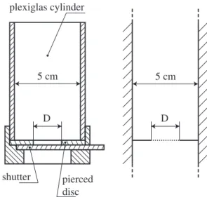
a e-mail: lionel.pournin@epfl.ch pierced disc shutter plexiglas cylinder D D 5 cm 5 cm
Fig. 1. The experimental setup we use to perform jamming trials (left) and its numerical model (right). The combination of the shutter with the pierced disc is modeled by a circular hole (dotted line) that can either be opened or closed.
to capture in its globality, even with stochastic model-ing which has so far not been successful. This paper re-ports on experimental investigations of the arching effect based on numerical simulation validated with trials using
confirms the simulation results, suggesting that distinct element simulation models allow for realistic reproduction of static granular phenomena.
Using the above setup, the jamming probability of a given bead assembly will be estimated as a function of the hole’s diameter D. In this way, we can determine the diameter ¯Dj of the opening hole for which the jamming
probability of this medium is 0.5. This diameter, called median jamming diameter is the quantity we use to char-acterize the tendency of an assembly of beads to jam.
Surface properties of the involved beads are charac-terized by their static friction coefficient µ. This paper first reports on numerical trials conducted using the Dis-tinct Element Method [8–11] with monodisperse bead as-semblies and several friction coefficients. Experiments per-formed on the same monodisperse assemblies composed of steel beads show that using those numerical models with a constant friction coefficient provides realistic values for
¯
Dj. Finally, measures of ¯Dj for bidisperse bead
assem-blies are obtained from simulations. Those results show that for a constant friction coefficient, ¯Dj only depends
on the beads’ volume-average diameter, which suggests that a law can be formulated about the jamming of poly-disperse bead assemblies.
2 The experiment
The setup we use to perform jamming trials is a plexiglas cylinder with interchangeable aluminum discs at the bot-tom that feature a circular hole in their centers. The inner diameter of the cylinder is 5 cm and the bottom discs have various diameters D for their central holes. The hole of the bottom disc can be obstructed using an aluminum shutter as shown on the left side of Figure 1.
The experiment proceeds as follows. First, the beads are poured into the cylinder while the hole of the bottom disc is obstructed by the shutter. The grains then pile up under the action of gravity and reach a mechanical equilibrium. Finally the shutter is suddenly pulled out and the medium either flows through the hole of the bottom disc or jams. From now on, we call Φ the bead diameter. For our experimental trials, we used steel beads with Φ = 1.0 mm, Φ = 4.0 mm, Φ = 5.0 mm and Φ = 7.0 mm. All trials were carried out using as close as possible to 0.575 kg of those steel beads, resulting in a filling height of around 6.5 cm independently of the bead diameters.
with the shutter acts as an uneven bottom in the experi-mental setup while its numerical counterpart is perfectly flat. Thus, removing the shutter in experimental trials ap-plies a shearing at the bottom of the granular piling. This is not the case in numerical trials where contacting forces suddenly disappear when the hole is opened. The numeri-cal wall friction coefficients are identinumeri-cal to the bead-bead friction coefficient, while friction occurs between steel, plexiglas and aluminum bodies in our experiments. Finally, the initial pourings of the beads in the numerical framework and in the experimental one are different. Sev-eral methods exist to prepare numerical pilings [12]. Those methods will produce initial situations that are often diffi-cult to achieve experimentally like spatially homogeneous polydisperse pilings. This is why we use a simplified ver-sion of the sedimentation technique [12]: we generate the beads randomly inside the containing cylinder, and move them downwards as close as possible to the bottom disc, in order to achieve a dense preliminary state. Then, we simply let the beads fall under the action of gravity from this state which is already dense enough for only few re-arrangements to be needed while the initial piling settles. In particular those rearrangements will not significantly disturb the spatial homogeneity of the preliminary state in the case of bidisperse assemblies. In the experimental procedure used for monodisperse sets of beads, the pour-ing is done from above the cylinder instead. This would produce segregation in the case of bidisperse media.
3 The median jamming diameter
A trial will either result in the observation “the medium jams” or “the medium flows”. We say that the medium flows if at the end of the experiment, none of the remain-ing beads has its center above the hole. By repeatremain-ing the experiment using several pilings composed of the same beads, one can estimate the probability for them to jam with a hole of given diameter. This allows in particular to find the statistical diameter ¯Dj of the opening hole
for which the jamming probability is 0.5. More precisely, ¯
Dj is statistically evaluated as the value below which the
opening diameter of flowing trials will lie with a probabil-ity of 0.5. In order to estimate ¯Dj, we process the results
using a generalized linear model [13]. Confidence intervals for ¯Dj are found by applying a bootstrap method [13].
A
B
C
(i)
(ii)
(iii)
Fig. 2.Views of actual trials. Snapshots (i) and (ii) are bottom views of numerical trials where the medium jams with parameters Φ= 6.0 mm and µ = 0.8 for (i) and Φ = 7.0 mm and µ = 0.0 for (ii). Beads denoted A, B and C in snapshot (i) are merely held by friction. Snapshot (iii) is a top view of an experimental trial with steel beads of diameter Φ = 7.0 mm where the medium flows, showing the formation of bead rings. All media are monodisperse.
(i.e. confidence intervals smaller than a tenth of prediction intervals) requires between 100 and 1000 trials. The 168 numerical estimations of ¯Djreported below required some
40000 trials and around 15 years computing time on a fast single-processor machine. We carried out our actual com-putations on several 2.7 GHz G5 PowerPC processors and on a cluster comprising 40 2.8 GHz Intel Xeon processors.
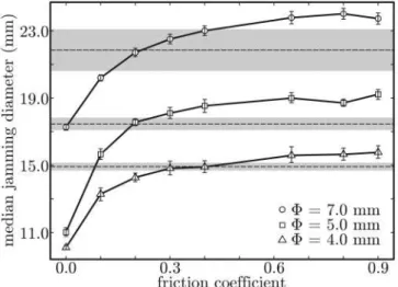
4 Influence of friction on jamming
The tendency of a powder to jam is known [14] to reflect the friction coefficient of its constituting particles. In our macroscopic framework, this is still the case as shown in Figure 3 for monodisperse assemblies with Φ = 4.0 mm, Φ = 5.0 mm and Φ = 7.0 mm. In particular, the me-dian jamming diameter is a globally increasing function of the friction coefficient. This dependence on friction is well marked for low values of the friction coefficient while it can practically be neglected for high ones. High frictions allow a wider range of jamming configurations than low ones because of a higher involvement of tangential forces in the stability of the system. Indeed, the possibilities for neighboring beads to carry each other are then more nu-merous. This results in larger arches and higher values of
¯
Dj, explaining the trend observed in Figure 3. Inversely,
low frictions yield way fewer arrangements, which are most of the time regular such as in Figure 2, (ii). Note that the values of ¯Dj obtained with Φ = 4.0 mm and Φ = 5.0 mm
are much closer for µ = 0 than for µ > 0. This will be explained below as a consequence of the formation of con-centric bead rings in the container.
The median jamming diameters measured from our ex-periments with steel beads are shown in Table 1 and plot-ted in Figure 3 for Φ = 4.0 mm, 5.0 mm and 7.0 mm. These results suggest that our steel beads can be simulated with a numerical friction coefficient µ that is approximately in-dependent of the bead size and lies between 0.2 and 0.3.
Fig. 3.The median jamming diameter obtained from numeri-cal trials as a function of the friction coefficient for Φ = 4.0 mm, Φ= 5.0 mm and Φ = 7.0 mm. Experimental values of Table 1 for Φ = 4 mm, Φ = 5 mm and Φ = 7 mm and their confidence intervals are reported on the graph respectively as dashed lines and greyed zones.
Table 1. Results of experimental trials on monodisperse sets of steel beads. Φ(mm) D¯j(mm) 1.0 3.88 ± 0.15 4.0 14.92 ± 0.23 5.0 17.46 ± 0.37 7.0 21.85 ± 1.24
This range will be discussed and refined below using ex-periments on bidisperse assemblies. Mind that these values certainly also reflect the differences between experimen-tal and numerical setups and further investigations are
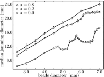
Fig. 4. The median jamming diameter plotted for simulated monodisperse media with several values of Φ and µ. Due to small numbers of data for Φ = 2.5 mm and 3.0 mm with µ = 0.0 and for Φ = 2.5 mm with µ = 0.8, the intervals shown are prediction intervals instead of confidence intervals and are represented as dotted lines.
needed to check their actual relevance regarding the real bead-bead friction coefficient.
Friction also highly influences the shape of arches. With cohesive particles, some authors suggest that arches in two dimensions have a globally circular shape [15,16]. With two-dimensional dry discs, arches are always con-vex in the frictionless case and may be non-concon-vex other-wise [17]. In three dimensions, the notion of convexity still has to be formally defined for granular arches. Yet, non-convex arches are easily recognizable. In particular, most of the arches we obtain with high frictions are non-convex: they feature beads that are held by tangential forces alone, as beads A, B and C in Figure 2. With frictionless beads, almost all the arches we observed seemed to be convex.
Measuring the Coulomb friction coefficient between pairs of steel beads is very complicated. In fact the friction coefficient usually measured is that between a sphere and a plane, using a tribometer or a tilted plane. In [18], the friction coefficient was measured with both methods for steel beads yielding values between 0.1 and 0.7 depending on surface conditions. Note that this range contains the interval 0.2 ≤ µ ≤ 0.3 obtained above with our beads. As suggested at the beginning of the section, our experiment could lead to an alternate way of determining the bead-bead friction coefficient. Carrying this to its maturity is a challenging subject for future work.
5 Jamming in monodisperse bead assemblies
Figure 4 shows ¯Dj plotted against Φ for numerical
monodisperse assemblies. One can see that ¯Dj(Φ) is nearly
linear for µ = 0.8. However, for frictionless beads, ¯Dj
fea-tures strong local non-linear behavior given by a sequence of significant drops for Φ > 4.75 mm. Observe now that for µ = 0.2, ¯Dj has a slight drop between Φ = 5.25 mm
Fig. 5. Bead rings diameters δi (dotted lines) and median
jamming diameters ¯Dj (solid lines) plotted for monodisperse
assemblies of beads. The median jamming diameters are shown for µ = 0.0 (lower curve) and µ = 0.2 (upper curve). The dashed lines τµshow the trend ¯Dj would follow for a friction
coefficient µ without the effect of the bead rings.
and Φ = 6.25 mm and then reaches a plateau. Irregulari-ties of ¯Dj actually also occur for non-zero friction, but for
larger bead diameters than in the frictionless case, and with lower amplitudes. We identify this non-linear behav-ior as a boundary effect. Indeed, the cylindrical shape of the container promotes the creation of concentric bead rings as shown in Figure 2, (ii) and (iii). This effect is especially strong for large beads and low friction coeffi-cients. Those rings disturb the linearity of ¯Dj(Φ) because
their ability to flow through circular openings is not the same as that of random arrangements. Indeed, if the ring has a diameter enabling it to flow freely through the hole, it does not represent an obstacle for other beads. On the other hand, if the hole diameter is slightly below the outer ring diameter, the beads of the ring in contact with the hole will collectively reduce its diameter by approximately two bead diameters. The above-mentioned non-linearities in the plot of ¯Dj against Φ nicely reflect this.
Call δi, i ≥1 the diameter of the i-th bead ring
mea-sured at the center of the beads and indexed from the boundary to the interior of the cylinder. At the end of each trial the bead rings appear clearly on the radial dis-tribution of the bead centers, and the values of δi, i ≥ 1
can be measured precisely. We plot them in Figure 5 for Φranging between 2.5 mm and 9.5 mm, together with the values of ¯Dj obtained for friction coefficients µ = 0.0 and
µ = 0.2. We observe that the ring diameters do not de-pend on the friction coefficient µ and that the distance between two consecutive bead rings is most of the time 5% to 10% smaller than the diameter of the beads. Some space is left empty within the rings due to the spherical shapes of their constituting beads. This can be noticed in Figure 2, (ii). Beads in adjacent rings will insert in this space in order to take advantage of the available volume in the best possible way, which reduces the distance between consecutive rings.
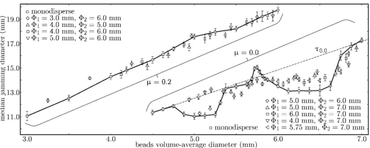
Fig. 6. Median jamming diameters obtained numerically for a selection of monodisperse and bidisperse bead assemblies. Top curve: µ = 0.2 and ¯Φranges from 3.0 mm to 6.0 mm. Bottom curve: µ = 0.0 and ¯Φranges from 4.5 mm to 7.0 mm.
For a given value of µ, call Φi the beads’ diameter so
that ¯Dj = δi. The points with coordinates (Φi, ¯Dj(Φi)) lie
on a same straight line τµ (see Fig. 5). Intuition suggests
that ¯Dj should increase as a function of Φ. This is not
the case except when Φ is close to Φi. Far away from Φi,
¯
Dj(Φ) decreases. There, the median jamming diameter is
constrained to remain between two consecutive bead rings and therefore follows the decreasing trend of their diam-eters. It seems likely that τµ would be the law ¯Dj would
follow without the effect of those periodic rings. Indeed, τµ extrapolates to large Φ the linear behavior ¯Dj has for
small Φ. In this light, the fact that ¯Dj(Φ) lies on τµ in the
neighborhood of Φi can be seen as a local disappearance
of the ring effect.
One can see in Figure 2, (iii), that rings form in our experiments with steel beads, corresponding to a simu-lated friction coefficient between µ = 0.2 and µ = 0.3. This shows that bead rings also occur in reality and not only in our numerical framework and further confirms that they indeed form with non-zero–friction coefficients. Re-call that the amplitude of the non-linearities of ¯Dj
de-creases with increasing µ. Friction promotes disorder and makes it more difficult for beads to arrange regularly, which smoothes the variations of ¯Djdue to the ring effect.
6 Jamming in bidisperse bead assemblies
Bidisperse media are characterized by two distinct bead diameters Φ1 and Φ2. We gather them into one single
pa-rameter, the volume-average diameter ¯Φof the beads:
¯ Φ=N1Φ 4 1+ N2Φ 4 2 N1Φ31+ N2Φ32 ,
where N1and N2are the number of beads with diameters
Φ1and Φ2, respectively. Measures of the median jamming
diameter have been performed for bead assemblies with
µ = 0.2 and ¯Φ ranging from 3.0 mm to 6.0 mm. The re-sulting median jamming diameters are plotted against ¯Φ in Figure 6 (top curve) together with the monodisperse results obtained with µ = 0.2. In this representation, bidisperse measures collapse on the monodisperse curve with very good accuracy. One has to be cautious though, for bidisperse media with Φ1 significantly smaller than
Φ2, yet close enough to ¯Φlike the measures obtained for
¯
Φ= 3.25 mm and ¯Φ= 3.75 mm with the mix Φ1= 3.0 mm,
Φ2= 6.0 mm. In those cases, the median jamming
diame-ters are statistically greater for bidisperse media than for monodisperse ones. This can be explained in terms of seg-regation. Indeed, such granular assemblies feature a small number of large beads that are significantly larger than the others. This leads to a strong tendency to segregate while the medium flows. Large beads actually migrate to the top and remain there while small beads flow through the hole. When the large beads finally reach the hole, most of the time they gather in an arch.
Otherwise, bidisperse and monodisperse results fit very well for µ = 0.2. This comes all the more unexpected since a monodisperse bead assembly defined using the volume-average diameter does not fill the same volume fraction as the corresponding bidisperse assembly. One can further observe that two bidisperse media with same
¯
Φ but different diameters for their constituting beads will have the same median jamming diameter. Those ob-servations lead us to formulate the following tentative law:
For fixed interparticulate friction, the median jamming diameter of spatially homogeneous bead assemblies only depends on their volume-average diameter.
With frictionless beads, the dependence of ¯Dj on the
diameter of the beads is strongly non-linear due to the influence of bead rings. Figure 6 (lower curve) reports re-sults of both monodisperse and bidisperse trials obtained with µ = 0.0 and ¯Φranging from 4.5 mm to 7.0 mm. One
on ¯Φ, but only on Φ2: for a given value of Φ2 the δi will
be equal to those obtained with monodisperse assemblies whose beads have diameters Φ = Φ2.
In the monodisperse case with Φ = 7.0 mm, the bead rings have diameters δ1 = 43.0 mm, δ2 = 29.96 mm and
δ3 = 16.52 mm (see Fig. 5). As discussed in Section 5,
¯
Dj tends to stay between two ring diameters. For
bidis-perse assemblies with Φ2 = 7.0 mm and ¯Φ close to Φ2
(that is ¯Φ ≥ 5.75 mm), ¯Dj then tends to stay below δ3
which explains why it remains constant for 5.75 mm ≤ ¯
Φ ≤ 6.75 mm. Here, ¯Dj follows the constant behavior of
the δi for the same reasons it follows their decreasing
be-havior in the monodisperse case.
Observe, though, that for ¯Φ ≥ 5.75 mm, all values of ¯
Dj measured on bidisperse assemblies with Φ2= 7.0 mm
collapse on the same curve. Now, consider the measures of ¯Dj obtained with mixtures Φ1= 5.0 mm, Φ2= 6.0 mm
and Φ1= 5.0 mm, Φ2= 7.0 mm (Fig. 6). For ¯Φ ≤5.75 mm,
one can see that they collapse on the same curve as well. Further observe that mixtures with Φ1= 5.0 are in
analo-gous conditions regarding the bead rings when ¯Φis close to 5.0 mm. This suggests that our law remains valid for bead assemblies submitted to the ring effect, provided that they are in identical conditions regarding ring formation.
Finally, one can see that the values of ¯Djobtained with
the mixture Φ1 = 4.0 mm, Φ2 = 7.0 mm collapse on τ0.0
for 4.9 mm ≤ ¯Φ ≤5.2 mm. Indeed, ¯Φis away from both Φ1
and Φ2, and the corresponding assemblies are bidisperse
enough to prevent ring formation.
Similarly to friction, the degree of polydispersity is a parameter that induces disorder in granular assemblies and makes it more difficult for such regular patterns as bead rings to build. When friction disappears, the degree of polydispersity becomes predominant in this role, and regulates the variations of ¯Dj as just discussed.
7 Experimental validation
In order to check the law formulated above, experiments with bidisperse sets of real beads were carried out. While it is easy to perform monodisperse experiments, bidis-perse ones turn out to be a lot trickier. Indeed, strong segregation can occur when pouring beads of two dis-tinct diameters into the initial piling of a trial and when the medium flows, it behaves like a succession of more or less thick monodisperse layers. Thus, much care is needed
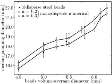
Fig. 7.Median jamming diameters obtained numerically and experimentally for 4.5 mm ≤ ¯Φ ≤ 6.25 mm. Experimental re-sults are obtained using bidisperse assemblies of steel beads with Φ1= 4.0 mm and Φ2= 7.0 mm. Numerical results are
ob-tained using monodisperse assemblies with friction coefficients µ= 0.2 and µ = 0.3.
Table 2. Results of experimental trials on bidisperse sets of steel beads with Φ1= 4.0 mm and Φ2= 7.0 mm.
¯
Φ(mm) D¯j(mm)
5.00 17.35 ± 0.93 5.45 18.50 ± 0.84 5.81 20.01 ± 0.93
when performing physical experiments. We use the follow-ing procedure: small bidisperse subsets of between 10 and 20 beads with the wanted volume-average diameter ¯Φare poured one after the other into the container. The latter is turned around its vertical axis by hundred twenty degrees between two consecutive pourings. The beads are poured gently to avoid that they mix with those that have already settled below. Preparing one such homogeneous bidisperse bead assembly takes approximately one hour.
The diameters of the steel beads constituting our experimental bidisperse media are Φ1 = 4.0 mm and
Φ2= 7.0 mm and three volume-average diameters ¯Φhave
been investigated: 5.0 mm, 5.45 mm, and 5.81 mm. Table 2 reports the median jamming diameters measured using those experiments. Comparing Tables 1 and 2, one can see that monodisperse steel bead assemblies with Φ = 5.0 mm and bidisperse steel bead assemblies with volume-average diameter ¯Φ = 5.0 mm have nearly identical median jam-ming diameters. This is a first experimental confirmation of our law.
The values of ¯Dj listed in Table 2 are plotted in
Figure 7 against ¯Φ, together with measures obtained nu-merically on monodisperse media with friction coefficients µ = 0.2 and µ = 0.3. One can see that experimental points lie close to both numerical curves. As discussed in Section 4, monodisperse results suggest that the nu-merical friction coefficient µ corresponding to our steel
beads should lie between 0.2 and 0.3. This is confirmed by Figure 7 and indicates that our simulation model is indeed able to reproduce static granular media. Moreover, the good agreement observed in this figure between the exper-imental bidisperse results and the numerical monodisperse ones provides a further validation of our tentative law.
8 Conclusion
Our experimental and numerical trials have resulted in an excellent agreement of the corresponding estimated median jamming diameters, thereby validating numerical simulation as an appropriate tool for the study of jam-ming. Furthermore, we have investigated the role of fric-tion and boundary condifric-tions on the median jamming di-ameter as a function of bead didi-ameters and identified the formation of bead rings as an important element therein. Finally we have studied bidisperse media and found (both by simulation and experiment) their jamming behavior to be characterized by their volume-average diameter over a wide range of granulometries. The following questions re-main open for future research: using our approach for ex-perimental determination of the bead-bead friction coeffi-cient, finding the influence of orifice and container shapes on jamming, and studying the dynamic interplay between segregation and jamming in order to refine the empirical law we formulate here.
This project was partially funded by the Swiss National Science Foundation, grant No. 200020-100499/1 and by arma-suisse. Many thanks to J. Bahar and S. Hold for carrying out the bidisperse experiments and to M.-O. Boldi for his statistical
guidance. Finally we want to express our appreciation for the insightful and stimulating remarks by the two referees.
References
1. W.A. Beverloo, H.A. Leniger, J. Van De Velde, Chem. Eng. Sci. 15, 260 (1961).
2. R.L. Brown, J.C. Richards, Principles of Powder Mechan-ics (Pergamon Press, 1970).
3. I. Zuriguel, L.A. Pugnaloni, A. Garcimartin, D. Maza, Phys. Rev. E 68, 030301 (2003).
4. I. Zuriguel, A. Garcimartin, D. Maza, L.A. Pugnaloni, J.M. Pastor, Phys. Rev. E 71, 051303 (2005).
5. R. Ar´evalo, D. Maza, L.A. Pugnaloni, Phys. Rev. E 74, 021303 (2006).
6. L.A. Pugnaloni, M.G. Valluzzi, L.G. Valluzzi, Phys. Rev. E 73, 051302 (2006).
7. L.A. Pugnaloni, G.C. Barker, Physica A 337, 428 (2004). 8. P.A. Cundall, O.D.L. Strack, G´eotechnique 29, 47 (1979). 9. J.-A. Ferrez, Th.M. Liebling, Philos. Mag. B 82, 905
(2002).
10. L. Pournin, A. Mocellin, Th.M. Liebling, Phys. Rev. E 65, 011302 (2002).
11. L. Pournin, M. Weber, M. Tsukahara, J.-A. Ferrez, M. Ramaioli, Th.M. Liebling, Granular Matter 7, 119 (2005). 12. K. Bagi, Granular Matter 7, 31 (2005).
13. A.C. Davison, D.V. Hinkley, Bootstrap Methods and Their Application (Cambridge University Press, 1997).
14. A. Gioia, Pharm. Technol., February 1980, p. 65. 15. G. Enstad, Chem. Eng. Sci. 30, 1273 (1975). 16. A.J. Matchett, Powder Technol. 171, 133 (2007).
17. K. To, P.-Y. Lai, H.K. Pak, Phys. Rev. Lett. 86, 71 (2001). 18. N.A. Pohlman, B.L. Severson, J.M. Ottino, R.M. Lueptow,