HAL Id: insu-01785426
https://hal-insu.archives-ouvertes.fr/insu-01785426
Submitted on 9 Apr 2019
HAL is a multi-disciplinary open access
archive for the deposit and dissemination of
sci-entific research documents, whether they are
pub-lished or not. The documents may come from
teaching and research institutions in France or
abroad, or from public or private research centers.
L’archive ouverte pluridisciplinaire HAL, est
destinée au dépôt et à la diffusion de documents
scientifiques de niveau recherche, publiés ou non,
émanant des établissements d’enseignement et de
recherche français ou étrangers, des laboratoires
publics ou privés.
Beyond equilibrium: re-evaluating physical modelling of
fluvial systems to represent climate changes
Edwin R.C. Baynes, Wietse van de Lageweg, Stuart Mclelland, Daniel
Parsons, Jochen Aberle, Jasper Dijkstra, Pierre-Yves Henry, Stephen Rice,
Moritz Thom, Frédéric Moulin
To cite this version:
Edwin R.C. Baynes, Wietse van de Lageweg, Stuart Mclelland, Daniel Parsons, Jochen Aberle, et
al.. Beyond equilibrium: re-evaluating physical modelling of fluvial systems to represent climate
changes. Earth-Science Reviews, Elsevier, 2018, 181, pp.82-97. �10.1016/j.earscirev.2018.04.007�.
�insu-01785426�
OATAO is an open access repository that collects the work of Toulouse
researchers and makes it freely available over the web where possible
Any correspondence concerning this service should be sent
to the repository administrator:
[email protected]
This is an author’s version published in:
http://oatao.univ-toulouse.fr/23430
To cite this version:
Chen, Fang and Allou, Alexandre and Douasbin, Quentin and
Selle, Laurent and Parisse, Jean Denis Influence of straight
nozzle geometry on the supersonic under-expanded gas jets.
(2018) Nuclear Engineering and Design, 339. 92-104. ISSN
0029-5493
Official URL:
https://doi.org/10.1016/j.earscirev.2018.04.007
Beyond equilibrium: Re-evaluating physical modelling of
fluvial systems to
represent climate changes
Edwin R.C. Baynes
a,⁎,1, Wietse I. van de Lageweg
a,2, Stuart J. McLelland
a, Daniel R. Parsons
a,
Jochen Aberle
b,g, Jasper Dijkstra
c, Pierre-Yves Henry
b, Stephen P. Rice
d, Moritz Thom
e,
Frederic Moulin
faGeography and Geology, School of Environmental Sciences, Faculty of Science and Engineering, University of Hull, Hull HU6 7RX, UK bDepartment of Civil and Environmental Engineering, Norwegian University of Science and Technology, Trondheim, Norway cMarine and Coastal Systems, Department Ecology and Sediment Dynamics, Deltares, Boussinesqweg 1, Delft, The Netherlands dDepartment of Geography, Loughborough University, Loughborough LE11 3TU, UK
eForschungszentrum Küste, Leibniz Universität Hannover/TU Braunschweig, Hannover, Germany
fInstitut de Mecanique des Fluides de Toulouse (IMFT), Université de Toulouse, CNRS-INPT-UPS, Toulouse, France
gLeichtweiß Institute for Hydraulic Engineering and Water Resources, Technische Universität Braunschweig, Braunschweig, Germany
A R T I C L E I N F O Keywords: Fluvial Climate change Physical modelling Review Floods Ecosystems A B S T R A C T
The interactions between water, sediment and biology influvial systems are complex and driven by multiple forcing mechanisms across a range of spatial and temporal scales. In a changing climate, some meteorological drivers are expected to become more extreme with, for example, more prolonged droughts or more frequentflooding. Such environmental changes will potentially have significant consequences for the human populations and ecosystems that are dependent on riverscapes, but our understanding offluvial system response to external drivers remains incomplete. As a consequence, many of the predictions of the effects of climate change have a large uncertainty that hampers effective management of fluvial environments. Amongst the array of methodological approaches available to scientists and engineers charged with improving that understanding, is physical modelling. Here, we review the role of physical modelling for understanding both biotic and abiotic processes and their interactions influvial systems. The approaches currently employed for scaling and representingfluvial processes in physical models are explored, from 1:1 experiments that reproduce processes at real-time or time scales of 10−1-100years, to analogue models that compress spatial scales to simulate processes over time scales exceeding 102–103years. An important gap in existing capabilities identified in this study is the representation of fluvial systems over time scales relevant for managing the immediate impacts of global climatic change; 101– 102years, the representation of variable forcing (e.g. storms), and the representation of biological processes. Research tofill this knowledge gap is proposed, including examples of how the time scale of study in directly scaled models could be extended and the time scale of landscape models could be compressed in the future, through the use of lightweight sediments, and innovative approaches for representing vegetation and biostabilisation influvial environments at condensed time scales, such as small-scale vegetation, plastic plants and polymers. It is argued that by improving physical modelling capabilities and coupling physical and numerical models, it should be possible to improve understanding of the complex in-teractions and processes induced by variable forcing withinfluvial systems over a broader range of time scales. This will enable policymakers and environmental managers to help reduce and mitigate the risks associated with the impacts of climate change in rivers.
1. Introduction
Global climate change is a grand challenge facing the Earth across numerous spatial and temporal scales (IPCC, 2014;EEA, 2017) and the
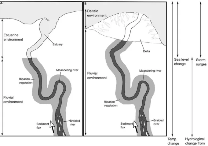
supply of water through the river networks is critically important for the Earth's population (de Wit and Stankiewicz, 2006). Expected im pacts of climate change influvial and fluvially affected systems such as river deltas and estuaries (Fig. 1) include altered hydrological regimes
⁎Corresponding author.
1Now at: Univ Rennes, CNRS, Géosciences Rennes - UMR 6118, 35000 Rennes, France. 2Now at: Antea Group Belgium, Roderveldlaan 1, 2600 Antwerp, Belgium.
and sedimentfluxes (Nijssen et al., 2001;Syvitski et al., 2005), varia tions in biota distribution and growth patterns (Harley et al., 2006), and more frequent extreme events such as storm surges (Lowe and Gregory, 2005), riverfloods (Garssen et al., 2015) and droughts (Garssen et al., 2014). Understanding and adapting to these potentially irreversible and detrimental impacts associated with new rates of environmental change and shifts in the frequency and magnitude of events associated with climate change is therefore a fundamental priority for potentially vul nerable fluvial environments, especially in regions where the human population are dependent on the local water supply (de Wit and Stankiewicz, 2006). In fact, management offluvial environments pre sents challenges in a changing climate, and requires an improved un derstanding of the feedbacks and interactions between the driving mechanisms at work.
Physical modelling is an important tool for research influvial sys tems and an established technique for the design and testing of hy draulic structures. The high degree of experimental control in physical scale models allows for the simulation of varied, or rare, environmental conditions and hence measurements of conditions which cannot be measured in the prototype (i.e. the real site to be modelled). Moreover, physical modelling provides an essential link between field observa tions and theoretical, stochastic and numerical models which are re quired to predict the impact of environmental changes on aquatic ecosystems (Thomas et al., 2014). Physical modelling can therefore play a key role in the development of a better understanding of climate change impacts by improving our ability to predict these impacts and, in turn, help adaptation to climate change related challenges (Frostick et al., 2011, 2014).
Physical scale models are a key tool to simulate and investigate complex processes and feedback mechanisms, with experimental
designs that reflect the spatial and temporal scale of the problem under investigation. Such techniques have been used for > 100 years to in vestigate the interaction amongst flow, sediment transport, mor phology, and interactions with biota, enhancing the understanding of many different and complex sediment transport and morphological processes across different spatial and temporal scales (Kleinhans et al., 2015).
Physical modelling for climate change adaptation faces the chal lenge of incorporating, and scaling, non linear responses across a range of temporal and spatial scales resulting from long term changes in event frequency and magnitude. Recently, physical models have started to explore the impact of climate change on the aquatic environment by examining boundary conditions that reflect a possible future climate state, often using a simplified representation of the systems (i.e. single grain size sediment, or no biotic elements). In addition to evaluating the behaviour of a system at thefinal stage of a future climate scenario, work is required that explores the progressive development of the system, including time varying processes, from one state to another as a consequence of climate change (IPCC, 2014;EEA, 2017). In particular, the morphology of riverine, deltaic and estuarine environments will develop and change over time in response to long term changing boundary conditions and process rates. To address the challenges re lated to climate change, it is crucial to develop a further understanding of the complexity of the systems, and how the environments adapt over longer periods of time, whether this change is gradual or sudden, and how they behave under a different climate regime.
In this context, this review will examine current techniques and capabilities in physical modelling experiments for representing climate change induced impacts on aspects offluvial systems such as hydro dynamics, sediment transport, morphodynamics and ecohydraulics. Fig. 1. Schematic diagram to highlight the environments within the scope of this review paper, with an estuarine environment shown in (A) and a deltaic en-vironment shown in (B). Potential climate change impacts in these systems are identified. SeeTable 1for details of expected changes in the environments induced by climate change.
Firstly, this review provides a technical discussion of different model ling approaches and the formal scaling laws that they obey (Section 2), before identifying the challenges that physical models face for re presenting variable forcing and the impacts of climate change within experiments (Section 3).Section 4provides detailed examples of recent innovative approaches at the forefront of the physical modelling in environmental systems and how these modelling approaches may be enhanced in the future.
2. Scaling approaches and challenges in representing different time scales in physical modelling
Fig. 2presents a schematic overview of different model types and their ability to replicate the relevant spatial and temporal scales of the prototype. In the discussion below, we explain the essence of each of these approaches, the scaling laws that they must successfully achieve and provide some examples of their application for the understanding offluvial processes and systems.
In scaled models, the time passes generally faster than in the pro totype, which makes them attractive for the study of climate change impacts. However, as will be outlined below, their design and the in terpretation of results can be challenging because the hydrodynamic time scales are generally quite different from those for morphodynamic fluvial adjustments (Tsujimoto, 1990), and the scaling of biota is even more uncertain. Models based on both geometrical and dynamic simi larity (i.e. by scaling important force ratios; see below) are a well es tablished approach for designing hydraulic structures at larger spatio temporal scales while distorted models (models with different geome trical scale ratios in the horizontal and vertical directions), and relaxed scale analogue models attempt to reproduce some selected properties of the prototype (Peakall et al., 1996).
The scaling laws used to design physical models can be derived based on a dimensional analysis (Buckingham, 1914;Barenblatt, 2003).
An important prerequisite for the design of a physical model is the dynamic similarity that ensures a constant prototype to model ratio of the masses and forces acting on the system (Einstein and Chien, 1956; Yalin and Kamphuis, 1971; Hughes, 1993; Frostick et al., 2011), i.e. that the derived dimensionless parameters are equal in model and prototype. Important force ratios defining these dimensionless numbers can be obtained by considering inertia, gravity, viscosity, surface ten sion, elasticity and pressure forces, respectively. A perfect dynamic si milarity for all possible force ratios cannot normally be achieved for model scales that deviate from the prototype scale since the samefluid (water) is normally used in both prototypes and models. This means that it is not possible to design a downscaled model so that the relative influence of each individual force acting on a system remains in pro portion between prototype and model as outlined by e.g.,Yalin (1971), Hudson (1979),de Vries (1993),de Vries et al. (1990),Hughes (1993), Sutherland and Whitehouse (1998), Ettema and Muste (2004) and Heller (2011). Scale models need therefore to be designed in a way that maintains important force ratios whilst providing justification for ne glecting other force ratios. Neglecting force ratios will result in scale effects if the model is operated at boundary conditions where the ne glected force ratios are important; in other words, there will be a di vergence between up scaled model measurements and real world ob servations. Scale effects become more significant with increasing scale ratio and their relative importance depends on the investigated phe nomenon (Heller, 2011), i.e. scale effects will have to be accepted.
In the following discussion of the different modelling approaches, it is assumed that the model studies are carried out with water as model fluid so that the ratio of fluid properties in model and prototype such as fluid density ρr, fluid dynamic and kinematic viscosity μrandνr, re spectively are equal to 1; the subscript r denotes the ratio between model (m) and prototype (p). Moreover, scale effects due to fluid temperature will not be considered although it is worth mentioning that Young and Davies (1991) used heated water (30 °C) in their Fig. 2. The relative application of different approaches for physical modelling, with different approaches being more appropriate for modelling processes over different spatial and temporal scales. Developed fromPeakall et al. (1996).
=
hr Lr (9)
i.e. the dynamics of the suspended load transport can only be modelled exactly using an undistorted model. Considering all scaling criteria, it is therefore only possible for one transport mode to be modelled following similarity criteria while the other mode will be affected by scale effects (Hughes, 1993). Nonetheless, physical model experiments that simulate both modes of sediment transport have been attempted (Grasso et al., 2009). If movable bed models need to be distorted, the distortions should not be so large that the type of sedi ment transport changes (i.e. from bed load to suspended load or vice versa).
When maintaining the similarity in sediment density (ρs,r= 1 or (ρs− ρ)r= 1), undistorted models fulfil the criteria given by Eqs.(3) to (5)while violating the fall velocity (Eq.(6)) and the grain Reynolds number criterion (Eq.(2)). The latter corresponds for this model type to Re⁎r= Lr1.5indicating that they should be operated in hydraulic rough conditions, i.e. Re⁎> 70, to avoid scale effects arising through viscous forces as Re⁎in prototype conditions will be larger than in the model. Recent work has indicated that the value of Re⁎> 70 to define hy draulically rough conditions may be overly conservative, with the value potentially as low as 15 being sufficient (Parker, 1979;Ashworth et al., 1994;Kleinhans et al., 2017). An important limitation of this type of model in regard to the scale factor arises from the requirement to scale the sediment with the same factor as the model length scale. If, for example, fine sand is already present in the field, fulfilling this re quirement could easily result in using sediments that are cohesive, which generates additional problems due to the different behaviour of cohesive sediments compared to a granular material. To minimize this problem, special materials may be used such as Ballotini® (non cohesive glass microspheres with diameters as small as 45μm) or different model types as described below.
2.3. Distorted physical models
Distorted models are characterised by different horizontal and vertical length scales so that Sr≠ 1 (Fig. 2). The distortion leads di rectly to scale effects in the flow field (see e.g.Lu et al., 2013;Zhao et al., 2013) and geometric similarity may be replaced by geometric affinity (De Vries, 1993). Distortion is not acceptable in a model where the vertical velocity components are important, but vertically distorted models are acceptable for uniform, non uniform and unsteady flow conditions with relatively slow vertical motion (Novak et al., 2010). For example, considering scale models of river reaches, the horizontal di mensions involved are commonly much larger than the vertical di mensions and this will lead to unrealistic scale models if the vertical scale ratio (hr) is selected equal to the horizontal length scale ratio (Lr) (De Vries, 1993). Additional care needs to be taken with regard to potential scale effects due to water surface tension if the water depth in the model is low (Hughes, 1993;Peakall and Warburton, 1996;van Rijn et al., 2011) or if the model is operated with varying background water
levels (e.g., to simulate tidal effects) because the effect of wetting and drying bank material will change its behaviour (e.g,Thorne and Tovey, 1981). The key issue in reproducing mobile bed morphology is sedi ment mobility. Particle size cannot be reduced to the same degree as the other x, y, z dimensions of the experiment relative to the prototype because properties such as incipient motion and cohesion of silt and clay are significantly different from those of sand and gravel (Lick and Gailani, 2004). Given the small water depth andflow velocities in this model type, sediment mobility is typically lower than in the prototype or may even be below the beginning of sediment motion. Three methods have classically been applied to overcome this issue (Kleinhans et al., 2014): i) a vertical distortion of the model leading to increased gradients and reduced surface tension effects (Peakall et al., 1996); ii) tilting of the bed, which further increases the gradient; or iii) the in troduction of lightweight sediment.
Vertical exaggeration of the model compared to the prototype has a range of effects on sediment transport, morphodynamics and resultant stratigraphy. Stronger bed gradients combined with small water depths affect the threshold for the beginning of sediment motion (Shields, 1936;Vollmer and Kleinhans, 2007), which cascades into differences in sediment sorting patterns between the model and the prototype (Solari and Parker, 2000;Seal et al., 1997;Toro Escobar et al., 2000;Wilcock, 1993;Peakall et al., 2007;Stefanon et al., 2010). In addition, it can be shown analytically that wavelengths, migration rates and amplitudes of river bars are a function of channel width to depth, sediment mobility as well as channel curvature, width variations and sinuosity (Struiksma, 1985;Seminara and Tubino, 1989;Talmon et al., 1995). This implies that any vertical distortion in the scale model will alter the morphology and resultant stratigraphy as seen in the prototype. The introduction of lightweight sediments results in similarity in both Re⁎ and Fr⁎ while violating intentionally the sediment density as well as the relative roughness criterion. As indicated by the name, this type of models makes use of model sediments with a lower density than the prototype sediment. For models focusing on bed load transport it may be rea sonable to relax the criterion defined by Eq.(6).Low (1989)found in experiments with lightweight materials of different specific densities 1 <ρs/ρ < 2.5 and a grain diameter of d = 3.5 mm that the specific volumetric bed load transport rate qswas related to v⁎r/vs,rby a simple power relation and that qs~ v⁎6and ~vs−5.Zwamborn (1966)argued that the Fr⁎ criterion (Eq.(3)) is essentially the same as the v⁎r/vsr criterion and that a good similarity in river morphology can be ex pected between model and prototype if the latter criterion is used to gether with an appropriate friction criterion and near similarity in Re⁎. More details in regard to the scaling laws considering or neglecting the fall speed dependency for such models can be found inHughes (1993) andvan Rijn et al. (2011).
Distorted physical models with vertical exaggeration have been used extensively in the past across a range of scales, including ex tremely large basin wide hydraulic models designed for engineering purposes. A notable example is the Mississippi Basin Model (MBM) constructed by the US Army Corps of Engineers (Fatherree, 2004); a physical model of the entire Mississippi river and its core tributaries at a horizontal scale of 1:2000 and a vertical scale of 1:100 (Foster, 1971). The MBM was used to study the dynamics of peaks of individualflood hydrographs within the Mississippi basin, such as identifying areas where levees would be overtopped during an expectedflood on the Missouri River in 1952 (Foster, 1971) and proved to be an invaluable tool in studying the storage and dynamic effects of backwater areas (Louque, 1976). The operating cost of the MBM and similar scaled basin models such as the Chesapeake Bay (Fatherree, 2004) or the San Francisco Bay Delta Tidal Hydraulic Model (Wakeman and Johnston, 1986), was impractical due to their size, but they demonstrated the ability to accurately replicate the dynamics of individualflood events within basins over large spatial scales that is impossible using reach scale physical models.
The mechanism for suspended sediment transport differs from the mechanism for bed load transport. This is reflected by the criterion defined by Eq. (6) corresponding to the ratio of settling velocity to shear velocity, i.e. the Rouse number, which is most important for suspen sion dominated models. Such models are more common in coastal modelling applications than in alluvial river studies and require the reproduction of the uplift of particles due to turbulence induced by waves or currents, and their subsequent transport in the water column. In this context it is worth mentioning that, in the case of waves, such models require the consideration of different physical parameters in Eqs. (2) (6) than fluvial bed load models, such as the characteristic velocity (gHb)−0.5 instead of the shear velocity v⁎ and the breaking wave height Hb instead of water depth h (Hughes, 1993).
Assuming Froude similarity for the flow and inserting the corre sponding hydraulic time scale given by Eq. (8) into Eq. (6) yields:
role vegetation can have in controlling bank erosion, river pattern formation and channel mobility under the simplest conditions (Gran and Paola, 2001;Tal and Paola, 2007;Tal and Paola, 2010;Braudrick et al., 2009;van de Lageweg et al., 2010;van Dijk et al., 2013a;Wickert et al., 2013). The addition of fine silica flour in the experiments of Peakall et al. (2007)andvan Dijk et al. (2013b)as thefinest sediment into the models as a representation of cohesive silt and clay in nature can also be considered an analogue reach modelling approach, and has been shown to lead to active meandering systems due to the added cohesion of incorporatingfine grained material (Peakall et al., 1996, 2007;Kleinhans et al., 2014). The addition of nutshells has been used to represent low density and highly mobile sediment acting asfloodplain filler (Tambroni et al., 2005;Hoyal and Sheets, 2009;van de Lageweg et al., 2016;Ganti et al., 2016). Similarly, a wide range of extracellular polymeric substances (EPS) has been introduced into models to re present biological cohesion (Hoyal and Sheets, 2009;Kleinhans et al., 2014;Schindler et al., 2015;Parsons et al., 2016). For example, EPS has been used in analogue delta experiments to increase the range of nat ural morphodynamics processes that can be reproduced, by increasing the cohesion of the sediment material (Hoyal and Sheets, 2009). The polymer sediment mix, developed at the ExxonMobil Upstream Re search Company (Hoyal and Sheets, 2009) performed best in the pre sence of clay and sand, and the deltas produced during the experiments had geometries characteristic of natural deltas composed of sandy non cohesive sediments, allowing experimental investigations of forcing factors such as sea level rise on channel mobility and shoreline dy namics (Martin et al., 2009).
Second, analogue landscape models represent the spectrum of scale models associated with the largest spatial and temporal scales shown towards the top right inFig. 2. Such models typically concern an entire landscape (e.g. delta or mountain range) and aim to explore its evolu tion across longer (e.g. geological) time scales. River delta landscape experiments provide an example of this type of scale model (Fig. 4). The analysis of these experimental data allowed the identification of a small, but significant, chance for the preservation of extreme events in the stratigraphy due to the heavy tailed statistics of erosional and de positional events (Ganti et al., 2011). This quantified understanding of the evolution of a river delta system under rising base level would only be possible using the analogue landscape modelling approach, where processes characteristic of larger delta systems are replicated and monitored at high spatial and temporal resolutions that would be im possible in thefield.
3. Challenges representing climate change impacts in physical models
The impacts of climate change, and more broadly, non constant forcing, will affect fluvial systems over a range of time scales. Increased magnitude of individual events to millennial scale shifts in long term forcing dynamics such as the total volume and seasonal variations in annual precipitation and changes in the biological characteristics could have dramatic impacts on the state and functionality offluvial systems (Wobus et al., 2010). This section identifies the current challenges in representing these impacts on thefluvial environment using physical models.
3.1. Differing timescales of morphodynamic and hydrodynamic processes Hydrodynamic processes usually occur at a much shorter time scale than morphodynamic processes and, as will be shown below, time scales related to different morphological processes do not necessarily coincide in physical models (Yalin, 1971). This can, in turn, result in undesired scale effects that become more significant with decreasing physical model scale (i.e. of the reproduction of the prototype) (Fig. 2). The determination of sedimentological time scales in movable bed models is difficult and often subjective. In fact, the sedimentological 2.4. Process focused physical models
Here we introduce the term process focused physical models (Fig. 2) to describe Densimetric Froude models that relax the similitude in Re⁎ (Eq. (2)) whilst maintaining similarity in Fr⁎ (Eq. (3)), but do not have a particular target natural prototype in mind. These models allow the investigation of the processes and generic planform morphologies such as channel braiding by reproducing fundamental sediment transport processes such as bedload transport and exploring the sensitivity of processes and morphologies to different experimental conditions. Bed sediment must be mobile in the bedload regime to replicate gravel bed rivers in nature and mobile in the suspension regime to replicate sandbed rivers, which is challenging due to cohesive effects for silt and clay if used to represent scaled down sand (Smith, 1998; Hoyal and Sheets, 2009). This class of models simplifies the representation of both discharge regimes and sediment properties using simple flow regimes (constant discharge or single events to represent annual floods) and a hydraulically rough bed to minimize scale effects, which conflicts with sediment mobility requirements. This conflict is generally solved by applying a poorly sorted sediment mixture in which the coarsest frac tion ensures hydraulic rough conditions (Peakall et al., 2007; van Dijk et al., 2012). Examples of process focused models include the experi ments aimed at river meandering by Friedkin (1945) and the braided river experiments by Ashmore (1988). Many practical applications of such models indicate their suitability in studying morphodynamic processes within river reaches as well as for coastal environments (Hughes, 1993; Willson et al., 2007; Kleinhans et al., 2014).
There is an overlap between distorted models and process focused models when similitude in Re⁎ may be close to specific natural protoype situations (Fig. 2). Similarly, the point at which a process focused model should be described as an analogue physical model is not always clear since it is not known when simplifications in sediment char acteristics or discharge regimes make model behaviour differ sig nificantly from a natural system.
2.5. Analogue physical models
The evolution of river morphodynamics over larger spatial and temporal scales is often investigated in so called analogue models (Davinroy et al., 2012), which are designed to represent larger proto type environments over longer periods of time (Fig. 2). Analogue models are designed to study analogies or ‘similarity of process’ be tween the model and prototype and are not designed to keep strict si milarity in the above scaling criteria (Hooke, 1968), although they can theoretically be classified according to the model types defined above. However, the aforementioned model types are generally stricter in terms of similarity criteria than analogue models for which the vali dation or “effectiveness” (Paola et al., 2009) depends on the judgement of similitude in bed sediment movement (Ettema and Muste, 2004) or on the operator due to the lack of a specific methodology for describing the degree of morphodynamic and stratigraphic similarity in model studies (Gaines and Smith, 2002). Yet, well designed analogue models have been shown to be an essential tool for studying morphodynamic processes and stratigraphic expressions across a wide range of spatial scales for different river channel morphologies and fluvially affected coastal environments (Bruun, 1966; Hudson, 1979; Peakall et al., 2007; Wickert et al., 2013; Green, 2014; Bennett et al., 2015; Yager et al., 2015; Baynes et al., 2018), despite violating the aforementioned scaling rules in many ways (Paola et al., 2009; Kleinhans et al., 2014; Peakall et al., 1996; Kleinhans et al., 2015).
Due to the large range in spatial and temporal scales covered by analogue models, two sub groups can be identified (Fig. 2). First, ana logue reach scale models are process focused physical models with an added degree of scaling relaxation. Examples include the introduction of alfalfa as vegetation into the models as a representation of vegetation effects in nature. A host of experiments has highlighted the important
time scale cannot be freely chosen as it results from the chosen scales of the other model parameters (Hentschel, 2007) and, hence, depends on which scaling criteria are intentionally violated. Moreover, there is the need to distinguish between different time scales for different mor phological processes such as individual grain movement (tsg,r) and the evolution of the bed surface in the vertical (tη,) and horizontal (tLr) directions, respectively. Corresponding time scales are presented in general terms in.
According toYalin (1971), the movement of an individual bed load grain is governed by the geometrical scale of the particle diameter d and the kinematic scale v⁎, respectively resulting in the time scales tsg,r defined by Eqs. (10) and (11), where Eq. (12) results from the addi tional requirement of similarity in Re⁎(Table 2).
Considering the temporal development of a movable bed surface in a physical model, different scales in the horizontal and vertical direc tions need to be taken into account. Forfluvial environments, the most common approach to derive the time scale for the formation of a mo vable bed surface is based on the comparison of the model response time to known prototype response times (Vollmers and Giese, 1972; Kamphuis, 1975;Einstein and Chien, 1956). This is typically achieved by considerations of the variation of the bed surface levelη in vertical direction with time and the volumetric sediment transport rate q, i.e.
the Exner equation (Paola and Voller, 2005; Coleman and Nikora, 2009). Thus, the corresponding time scale can be defined according to Tsujimoto (1990)andHughes (1993):
= −
t L h (1 ϕ) q
ηr r r r
r (10)
whereϕ denotes the porosity of the bed material. A similar formulation can be obtained considering the movement of river dunes assuming their geometrical similarity in model and prototype. Introducing the dimensionless volumetric bed load transport rate q⁎= q/(v⁎d), Eq. (10)can be rewritten according to:
= − ∗ ∗ t L h (1 f) q d v ηr r r r r r r (11)
Assuming similarity in q⁎in model and prototype (i.e. q⁎r= 1), Eq. (11)represents the basis for Eqs. (12) to (15) inTable 2for which it was assumed that v⁎r= (hrSr)0.5= hrLr−0.5. Note that for geometrically si milar grains with a similar grain size distribution, (1− ϕ)r= 1 (Hentschel, 2007). Also, for practical purposes, the sediment transport rate is often determined from existing bed load formulae. Using such relationships in Eq.(11), instead of a measured q⁎, can result in dif ferent time scale calculations.
Eq. (16) inTable 2was derived byYalin (1971)and describes the time scale related to the evolution of the mobile bed surface in hor izontal direction. This equation is based on single grain movement considerations and the relation of the diameter scale with the long itudinal scale.
Comparing the different time scales given inTable 2 it becomes apparent that
< < <
tηr tLr tr tsgr (12)
i.e. the vertical evolution of the bed surface has the shortest time scale, followed by the longitudinal displacement of the grains and the hydrodynamic time scale. The longest time scale is for the individual motion of a grain (Peakall et al., 1996). Other time scales than those discussed here may be derived based on the consideration of the evo lution of morphodynamic features such as meander bend migration rate,floodplain evolution and biological development (Tal and Paola, 2007;Kleinhans et al., 2014, and references therein).
The time scales can also be linked to the bed load models defined above. In undistorted similarity models with unidirectional flow tsg,r= tηr= tLr= Lr0.5, which is equal to the hydraulic time scale tr. Geometric similarity models therefore offer the opportunity to study the effects of hydrographs on bed evolution. The time scales for distorted lightweight models can be derived as tsg,r= (ρs ρ)r2/3, tηr= hr3(1− ϕ)r (ρs− ρ)r−2/3, tLr= hr2(ρs− ρ)r−1 thereby assuming qr⁎= 1 and that bed shear stress can be determined from the depth slope product.
The time scales for process focused models are defined by Eqs. (14) and (15) where the latter formulation byTsujimoto (1990)was derived by considering the Manning equation, i.e. by considering additional similarity in bed roughness. Time scales for models with suspended load were summarized by e.g.Hughes (1993)andvan Rijn et al. (2011), but in almost all cases a morphological time scale of suspended models was derived corresponding to tηr= hr0.5 (where the vertical length scale characterizes wave characteristics). These similarity conditions can result in rather impractical scaling ratios, especially when considering both vertical and horizontal directions, and result in a challenge in developing strictly scaled models containing both sediment and water. 3.2. Representing variable forcing and sequences of events
Future climate regimes are anticipated to be characterised by in creased variability and higher frequency and magnitude of extreme events such as riverflooding (Table 1,Fig. 5). Due to the difficulties in scaling unsteadyflows and sediment transport in physical models (see Fig. 4. Example of an experiment using an analogue-landscape modelling
ap-proach (Sheets et al., 2002;Ganti et al., 2011). (a) Schematic of the experi-mental set up. (b) Photography of the delta after 11 h of experiexperi-mental run time. FromGanti et al. (2011).
Section 3.1), there are few physical modelling studies exploring se quences of multiple floods (e.g.Braudrick et al., 2009). In terms of improving our understanding of the impact of climate change onfluvial environments, it would be particularly relevant to investigate variations in hydrograph characteristics (i.e. duration, magnitude and frequency) over time scales that are similar to the system recovery time for mor phodynamics and vegetation. All systems have a characteristic time scale for recovery following a perturbation (Brunsden and Thornes, 1979). This time scale can range from > 103years in erosive bedrock settings (e.g. canyons;Baynes et al., 2015) to 101 102years in alluvial depositional fluvial environments (e.g. sandur plains; Duller et al., 2014) due to the relative differences in the mobility of sediments, al though larger systems typically take longer to fully recover following a perturbation (Paola, 2000). This illustrates that the timing of sequences offlood events relative to the time scale of recovery is as important in driving evolution and change influvial environments as the magnitude of individualflood events (Fig. 5). With an increased frequency of ex treme events, this recovery timescale may be threatened, with sub sequent events of possibly greater magnitude occurring before the system has fully recovered from the initial perturbation with potentially unknown consequences. Thus, the accurate representation of non con stant forcing and the relative importance of sequences of events within physical models remains an important goal for the development of the
understanding offluvial system response to future climate scenarios. Additionally, non linear threshold driven sediment transport processes which respond to constant or non constant forcing can destroy or “shred” environmental signals, like river avulsions or bar deposits, which could otherwise be preserved in the landscape or sedimentary record (Jerolmack and Paola, 2010). Changes in the external forcing may not be preserved if the timing and magnitude of the events does not exceed the autogenic variability driven by non linear processes such as bedload transport or river avulsion (Jerolmack and Paola, 2010). As the signal of the external forcing increases in frequency (e.g.,Fig. 5), preservation of the impact of the individual events becomes less likely, whilst events of sufficiently large magnitude will change or modify the entire system and will therefore have greater potential to be preserved (Jerolmack and Paola, 2010). If the evidence for changes in external forcing are not recorded or visible in natural systems, physical models provide a unique opportunity to understand how thresholds and auto genic feedbacks within a system can mitigate or enhance the impact of variations in external forcing driven by climate change.
Traditionally,flood events are represented in physical models at the event scale by triangular hydrographs with possibly an asymmetry between the rising and falling stages (e.g.Lee et al., 2004). The gradual increase and decrease of discharge are reproduced by stepped hydro graphs with the number of steps for each hydrograph strongly Table 2
Time scales for bed load dominated models,ρr=μr=νr= 1, and assuming v* = (ghS)0.5.
Time scale Eq. Criteria and comments Source
tsg, r= drLr0.5hr 1 (10) - individual grain movement Yalin (1971)
tsg, r= Lrhr 2 (11) - individual grain movement Yalin (1971)
- similarity in Re⁎
tηr= Lrhr (12) - similarity in dimensionless transport rate Yalin (1971)
- similarity in Re⁎
- porosity equal in model and prototype
tηr= Lr1.5dr 1(1 ϕ)r (13) - similarity in dimensionless transport rate Hentschel (2007)
tηr= Lr2.5hr 2(1 ϕ)r(ρs ρ)r (14) - similarity in dimensionless transport rate Hentschel (2007)
- similarity in Fr⁎ = − − tηr L hr r1.5dr (1 ϕ) 7 6 r
(15) - similarity in dimensionless transport rate Tsujimoto (1990)
- similarity in Fr* - near similarity in Re*
tLr= Lr1.5hr 1 (16) - individual grain movement Yalin (1971)
Table 1
Details of expected climate change induced impacts onfluvial and fluvial-affected estuarine and deltaic environments. Physical modelling studies can be used to understand these processes and test possible adaptation strategies.
Climate induced change in forcing
Predicted change Associated impact on estuarine andfluvial environments Source
Global mean surface temperature
By 2100:
0.3–1.7 °C temp. Rise (scenario RCP2.6a)
2.6–4.8 °C temp. Rise (scenario RCP8.5a)
Implications for vegetation growth in all environments IPCC (2014)
Sea level rise By 2100:
0.26–0.55 m (scenario RCP2.6) 0.45–0.82 m (scenario RCP8.5)
70% of coastlines worldwide experience change within 20% of global mean
Drowning of estuarine environments. Encroachment of saline water and associated impacts on biota. Increased aggradation of river deltas, accelerated channel and floodplain deposition and to higher channel avulsion frequency
IPCC (2014), Jerolmack (2009)
Storm surges Largest increase in 50 year return period storm-surge height at UK coastline = 1.2 m (Scenario A2)
Increased risk from hazards (e.g. coastalflooding, coastal erosion) associated with storm surge events
Lowe and Gregory (2005) Precipitation Scenario RCP8.5: Increase in mean precipitation in high
latitudes and equatorial Pacific. Decrease in mean precipitation in mid-latitudes. Increase in extreme precipitation over most of mid-latitude landmasses and wet tropical regions become more intense and more frequent
Rivers: increased frequency and magnitude of higher peak flows, and possible prolonged drought periods with associated impacts for riparian vegetation distribution. Potential shifts in timing of seasonal hydrological regimes
IPCC (2014),Garssen et al. (2014, 2015)
Waves Latitude dependent:
0.6–1 m increase in 20 year return period wave height between 1990 and 2080 in NE Atlantic. Wave with 20 year return period in 1990 will have 4–12 year return period in 2080
Modification of the dynamics of estuarine and coastal systems
Wang et al. (2004)
a
RCP2.6 and RCP8.5 refer to two end-member Representative Concentration Pathways for anthropogenic greenhouse gas emissions. RCP2.6 refers to a stringent mitigation scenario, and RCP8.5 refers to a scenario with very high greenhouse gase emissions (IPCC, 2014).
dependent on the complexity of theflume control equipment (Lee et al., 2004;Ahanger et al., 2008). Sequences offlood events modelled on a particular system, or the long term evolution of a system driven by a long term shift in the magnitude or frequency of forcing are rarely re presented in physical models (Fig. 5).
3.3. Representing biology and timescales of biological change
Currently, most hydraulic facilities are not well suited to work with living organisms. These facilities may therefore result in biota being stressed by one or more environmental factors including inappropriate water chemistry (salinity, pH, dissolved oxygen, inorganic carbon), water temperature, substrate (physical and chemical properties, soil saturation), lighting (composition, intensity, timing), and flow char acteristics (depth, velocity, drag). The health and behaviour of living plants may also be affected by biological considerations, including in sufficient nourishment (type, quantity, and timing), competition for resources amongst individuals and, potentially, the introduction of pathogens. Johnson et al. (2014a) provide a review of these main stressors and their management influme facilities. Of course, plants are often stressed in their natural environment by competition for resources and by other ecological and biological interactions. Their interactions with their environment are variable and complex, such that there is no ideal stress free state that must be mimicked. Nevertheless, a basic goal of most experimental work will be to reproduce in theflume behaviours that are typical in nature and, in that case, low levels of stress are
desirable, or the development of surrogates that accurately replicate plant/microbial activity and can be time scaled.
Most plants are able to tolerate a range of environmental conditions, with fatality beyond limiting thresholds. As conditions become less optimal, but sub lethal, the plant will adapt, potentially altering the way in which it interacts with theflow. We know very little about these adaptations and what they mean for hydraulic performance, but ex isting work suggests that the relations are likely to be complex, espe cially where multiple stressors are present (Puijalon et al., 2007).
Demonstrating that vegetation is not physiologically or behaviou rally stressed during experiments should be a standard element of any physical modelling experiment involving live plants. Without that as surance it is difficult to be confident that measured hydraulic and morphodynamic responses can be properly assigned to treatment ef fects, not abnormal behaviour caused by the physical modelling en vironment. While it may be relatively easy to detect serious ill health or the death of a plant that is part of aflume experiment, earlier stages of decline that affect the plants interaction with the flow, may go un detected, potentially undermining the results obtained.
This leads to the identification of two key challenges for in vestigating plantflow sediment interactions: i) developing protocols that can be used to monitor plant health or stress levels during physical modelling experiments, and ii) developing a fuller understanding of how health and stress levels affect key plant structures, physiological responses and behaviours that are relevant toflow and sediment in teractions. Meeting these challenges would provide a basis for making Fig. 5. Conceptual diagram indicating different forcing regimes in fluvial and fluvially-affected systems such as river deltas and estuaries under climate change. (A) A progressive increase in a constant forcing over a long time scale (e.g. sea level rise, or increase in biostabilisation as a result of temperature increase). (B) A forcing regime characterised by infrequent and low-magnitude extreme events, superimposed on the progressive trend shown in (A). (C) A forcing regime characterised by higher magnitude extreme events, but of the same frequency, compared to (B). (D) A forcing regime characterised by extreme events of the same magnitude as (B), but occurring more frequently. (E) A forcing regime characterised by extreme events that are both more frequent and of a higher magnitude compared to (B). The typical time for the system to recover back to equilibrium conditions is shown in grey in (B-E). Due to frequency and magnitude of the extreme events in (E), the system has never fully recovered before the subsequent extreme event, placing the system in a constant state of transience.
explore the behaviour of targeted processes under controlled conditions (Bonnet, 2009). The freedom given by foregoing the strict scaling laws can potentially allow innovative experiments to develop an under standing of systems that are manipulated in ways that would not be possible using a strict scaling approach, such as coastal dynamics and response to sea level rise (Kim et al., 2006) or the exploration of dif ferent sequences of events on the overall system behaviour (e.g.,Ganti et al., 2011). It is important to note that analogue models are ex clusivelyfit for these “thought provoking” experiments and hence our primary tool for investigating processes, interactions and feedbacks across longer (> 102years) time scales relevant for climate adaptation purposes (Fig. 2).
Intermediate time scales (101 102years) have proven difficult to represent in physical models to date, leaving us with a timescale gap in physical modelling capabilities. Yet, in the context of climate change adaptation for planning and policy purposes, the evolution offluvial systems due to climate change over intermediate time scales is most prevalent and urgent (Fig. 2). Depending on the exact timescale or process of interest, undistorted, distorted and process focused models may provide physical scaling approaches to study thefluvial system at hand. Undistorted and distorted scaled models are best suited to in vestigate individual and short lived events due to the minimum com pression of spatial and temporal scales (Fig. 2) extending the individual event scale covered by 1:1 models. Similarly, process focused and perhaps some distorted and analogue reach physical models are best placed to condense the timescales represented in analogue models in an effort to study the effects of intermediate timescales of climate change influvial systems (Fig. 2) the effects of variable forcing, sequences of events and biological interactions are dominant (Garssen et al., 2015) but poorly understood drivers of fluvial system behaviour for re searchers to be able to study the effects of climate change across in termediate timescales. Below, we provide examples of studies on vari able forcing, sequences of events, lightweight sediment and biology and we discuss how they can be applied to better represent climate change at intermediate timescales specifically and expand the future physical modelling capability more generally.
4.2. Variable forcing and event sequences
Recently,Martin and Jerolmack (2013)have advanced the knowl edge of bedform dynamics for non stationaryflows, including the dif ference in the scaling of morphodynamic and hydrodynamic processes (Section 3.1). The processes associated with the growth of bedforms following an abrupt increase in discharge and their decay following an abrupt decrease in discharge are complex and very different (Martin and Jerolmack, 2013). The former relies on gradual collision and merging of small structures towards larger ones, while the latter relies on the formation of secondary small scale structures that cannibalize progressively the large structures formed earlier during the rising stage (Martin and Jerolmack, 2013). The timescale of the bedform response under these conditions is proportional to the reconstitution time, de fined as Tr= V/qswhere V is the volumetric sediment displacement for the bedform adjustment and qs is the sediment flux (Martin and Jerolmack, 2013). The reconstitution time is a function of the equili brium bedform heights, and celerities under the initial and secondary discharge magnitudes, such that taller and longer bedforms take longer to return to equilibrium following an abrupt change in discharge.
Additionally, the mechanism and characteristics of the forcing change (i.e., discharge) was found to be important in setting the me chanism of bedform response on the channel bed (Fig. 6). Dependent on the rate of a gradual increase and decrease in the discharge (Fig. 6a b), bedforms either respond through a phase of hysteresis or through a linear response of the length and height (Fig. 6c f). Under the‘fast flood wave’ conditions, the timescale response of the bedform adjustment is shorter than the timescale offlood wave discharge, forcing the hys teresis response. These observations following their experiments under objective decisions about how stressed a plant is and whether the level
of stress is sufficient to affect its biomechanical behaviour as that affects its interactions with the flow and therefore the integrity of an experi ment.
From a scaling perspective, of primary interest is the role of the hydraulics as a driving force for the growth and, hence, the geometrical and mechanical properties of plants and biofilms. Hydrological mod ifications, driven by climate change, especially in terms of flood in tensity and frequency, are very likely to also modify plant diversity and distribution (Garssen et al., 2015). Importantly, the time scales asso ciated with plant and biofilm growth in the field are very large when compared to the time scales of physical modelling experiments in the laboratory. For photosynthetic biofilms in rivers, for example, growth cycles are associated with time scales of around 30 days, which corre lates approximately to inter flood periods in the field (see e.g. Boulêtreau et al., 2010). Macrophytes or riparian vegetation generally develop and grow over much longer time scales. For biofilms, another issue is the extreme versatility of this biological agent, whose growth and composition adapts very quickly to flow conditions during growth; for example, Graba et al. (2013) demonstrated that in steady flow growth experiments the biofilms optimized their mechanical properties to fit the imposed steady forcing, and were very easily detached by a slight increase of flow velocity. Incorporating flow unsteadiness asso ciated with typical discharge fluctuations then becomes important for growing representative laboratory biofilms.
Plants and biofilms can be simplified and represented by some physical or chemical surrogates. As far as plants are concerned, the use of physical surrogates offers the opportunity to better control the in teractions between aquatic vegetation and a changing hydraulic en vironment, without the issue of phenotypic plasticity typical from biotic systems (Read and Stokes, 2006; Nikora, 2010). However, the devel opment of surrogates relies on the good understanding of the plant biomechanical properties and requires therefore extensive field data collection prior to the main experiments (Nikora, 2010). Although re cent works are relying more and more on plant surrogates (see Johnson et al. (2014b) for a non exhaustive list), only a few studies investigated the surrogate design process for complex shaped aquatic plants, such as the work carried out by Paul and Henry (2014), and this process is yet to be developed for freshwater aquatic vegetation.
4. Innovative approaches and required future developments to represent climate change impacts in physical models
4.1. Bridging the timescale gap
The range of physical modelling approaches highlighted in Fig. 2 have worked well for both small and large spatial and temporal scales. At the event scale, 1:1 physical models have proven invaluable tools to examine the effects of storm wave on flooding risk and safety (Fig. 3). More extreme storm wave and river flood events are projected as a result of climate change (Table 1). The current hydraulic facilities are however expected to incorporate these more extreme events in their experiments seamlessly by adjusting their test scenarios to include the latest climate projections (e.g., wave height). Other than potentially running into size limitations of the hydraulic facility (i.e. larger events require larger facilities for 1:1 modelling, such as the Mississippi Basin Model; Foster, 1971), these more extreme events do not require addi tional scaling compared to default extreme event tests. This observation indicates that no problems are foreseen in representing more extreme events associated with climate change in hydraulic facilities.
Also at larger spatial (landscapes) and temporal (> 102 years) scales, analogue models have worked well leading to agenda setting research and understanding of landscape evolution processes (Hasbargen and Paola, 2000; Turowski et al., 2006; Tal and Paola, 2007; Bonnet, 2009). Analogue models can act as a tool for exploration, due to the ability to simplify aspects of a complicated system and
variable forcing allowed Martin and Jerolmack (2013)to propose a simple model framework for the quantitative prediction of bedform adjustment timescale and the occurrence of bedform hysteresis in nat ural rivers during individual or sequences of events. This innovative example demonstrates the future potential for physical models in ad vancing the understanding of the processes and response of fluvial systems under variable forcing conditions, aiding the understanding of the possible impacts of climate change. The identification of response timescales of morphodynamic processes to individual events (i.e., Martin and Jerolmack, 2013) can act as a starting point for evaluating the response to sequences of multiple events of different frequencies and magnitudes (Fig. 6).
The order of events can also be important for experiments in vestigating the impact of sequences of events, due to differences in sediment transport rate for flood events of different magnitude and duration. However, the reorganisation of bed morphology either in terms of bedform size or bed structure through events will impact on
the state of the system for the next event, which means that the order of events could be significant and this should be addressed in flume ex periments that investigate longer time scales.
4.3. Lightweight sediments
Lightweight materials have been used to study local erosion pro cesses such as scour development downstream of weir structures (e.g., Ettmer, 2006, and references therein), bridge piers and abutments (Fael et al., 2006;Ettmer et al., 2015) and the impact of jets (e.g.Rajaratnam and Mazurek, 2002). The latter studies, in particular, made use of the fact that erosion processes are accelerated when lightweight sediments are used instead of naturalfluvial sediments, i.e. that the equilibrium dimensions of the scour can be reached faster, allowing the time scales of study to be extended (Fig. 2). At a larger scale,Willson et al. (2007) reported on a distorted scale model focusing on river and sediment diversions in the lower Mississippi river delta with Lr= 1:12,000 and hr= 1:500 and a model sediment with a density ρs= 1050 kg/m3 covering 77 river miles and an area of about 3526 square miles. In this model, theflow was scaled via the Froude law and the lightweight sediment was scaled based on considerations for the incipient motion of the particles so that incipient motion and resuspension were similar in model and prototype. The resultant sediment time scale was given by the authors with 1:17,857 (one year of prototype time equals roughly 30 min of model time). This model was run for different scenarios, in cluding sea level rise, and used to enhance the general understanding of the impact of planned measures for US State and Federal Agencies (Willson et al., 2007). Such approaches, specifically using lightweight sediment to reduce the time scale of the environmental processes in the physical models can extend the timescale of scaled models (Fig. 2) to bridge the gap in modelling capabilities over the timescale relevant for climate change.
4.4. Representing biology
Time scales associated with the growth and behaviour of vegetation are inherently difficult to downscale in physical models using un distorted or distorted models. Therefore, it is more convenient to use living or artificial surrogates within the analogue modelling approach, where the effects of vegetation in the system are replicated, but not necessarily directly. Plant surrogates also offer new possibilities to test hypotheses in the context of changingfluvial systems.Johnson et al. (2014b)detailed the various benefits and the limitations of using inert physical surrogates, and these points will therefore not be detailed here. Yet, surrogate development is still in its infancy and depends on a de tailed knowledge of the morphology and biomechanics of the species of interest, and we present here some of the major issues yet to be tackled, in the context of changingfluvial systems.
The morphology and mechanics of aquatic plants can vary based on seasonal patterns. Influme experiments, the potential interaction be tween the different time scales such as the seasonal growth and the time between active and inactive hydrological regimes needs to be con sidered. In the case of experiments involving time compression (ana logue or process focused models always active/inflood, see e.g.Paola, 2000) effects due to seasonal changes of plant characteristics may be lost. A good understanding of the plant biomechanical properties re quires the use of a solid dataset from real life conditions (Nikora, 2010), collected using well identified techniques (Henry, 2014, 2018). Ad ditionally, the required level of complexity of a plant surrogate is still uncertain, as it is critical not to simply redesign the plant structure (Denny, 1988). Understanding the existing structural organisation of a plant is key to the identification of the environmental factor that de fined it, and should highlight the features to be reproduced in an ex periment, depending on the processes and scales to be investigated. The most important part in a design process, i.e. performance tests, should be conducted systematically to ensure that the dynamic behaviours of Fig. 6. Comparison of bedform dynamics under different variable discharge
regimes. (a) Hydrograph simulating a slowflood wave. (b) Hydrograph simu-lating fastflood wave. (c–d) Evolution of bedform height during the hydro-graphs. (e–f) Evolution of bedform length during the hydrohydro-graphs. A clear hysteresis is apparent in the evolution of the bedforms during the fastflood wave, due to time lag of response of the bedforms is greater than the timescales of theflood waves. Adapted fromMartin and Jerolmack (2013).
Schuurman et al., 2013;Liang et al., 2016), sediment vegetation in teractions in these systems (van Oorschot et al., 2016), and the evolu tion of coastal barrier systems (Castelle et al., 2013). Using datasets from the Barrier Dynamics Experiment (BARDEX II;Masselink et al., 2013), allowed the testing of existing numerical models and to identify priorities for their existing development in order to reproduce processes such as onshore/offshore sandbar migration (1DBeach model,Castelle et al., 2010), barrier erosion sequences (XBeach model;Roelvink et al., 2009) and the impacts of overtopping (SURF GN model; Bonneton et al., 2011). Testing of numerical models against physical modelling datasets could increase the confidence in numerical simulations, im proving the capability to model climate change adaptation. It may be noted that the development of the use of inert plant surrogates may also help and be done in parallel to numerical modelling studies replicating fluid flow around vegetation (Marjoribanks et al., 2014, 2015), whose effects can be included into larger numerical simulation addressing fluvial adaptation at a larger space and time scale.
Numerical models can be used to explore which combinations of variables are most worth studying in physical experiments and can aid with the planning of such experiments. Once accurately parameterised and calibrated in physical models, process based numerical models could be upscaled to cover larger spatial scales and longer time periods that are appropriate for climate change adaptation (i.e. intermediate scales). Also, numerical model simulations can be useful predictive tools because they can cover multiple spatial and temporal scales and they can easily be forced with a multitude of climate change scenarios that would be impractical using physical models. However, these nu merical simulations often contain associated uncertainty due to the inability to determine whether the observed behaviour is a result of true landscape dynamics or merely an artefact of the model set up. Physical models could potentially improve this confidence by replicating some of the same scenarios and comparing the behaviour and interactions between processes in both the numerical and physical simulations.
5. Conclusions
Physical modelling has contributed significantly to our under standing offluvial systems. This is expected to continue into the future as different physical modelling approaches are well suited to investigate the response and potential adaptation to climatically driven changes in forcing over various timescales. Based on a review of the state of the art in physical modelling offluvial systems, this study highlights that: (i) physical modelling offers a prime opportunity for furthering the current understanding of variability of forcing influvial systems. (ii) For the policy focused studies offluvial systems undergoing climate change adaptation, the modelled time scales using 1:1, undistorted or distorted scale models need to be extended and the modelled time scales using process focused or analogue models need to be reduced to address is sues relevant to decadal timescales. (iii) Representing the response of plants and organisms to changing conditions and the resulting feedback on physical processes requires more attention and better techniques than presently available, using both distorted scale and analogue sur rogate modelling approaches. (iv) Coupling of physical modelling output with numerical model parameterisation and development is crucial for producing accurate predictions of howfluvial systems will respond in the future to a range of possible forcing scenarios over multiple time scales.
Within the context of climatic change influvial environments, fu ture focus and investment is recommended towards the physical mod elling of the detailed interactions between riverine biology, hydrology and morphology, non constant forcing and an understanding of the impacts of single events, multi decadal oscillations and longer term trends. This will enable the development of appropriate and effective mitigation strategies for fluvial ecosystems and environments under threat from climate change, that are grounded in robust physical ex perimentation.
Acknowledgments
We thank Jeff Peakall and one anonymous reviewer for the Fig. 8. Effect of extracted extracellular polymeric substances (EPS) content on bedform morphology. (a) 0% EPS, (b) 0.125% EPS content, (c) 1% EPS content. (d) Ripple height development for different EPS contents (black: 0%, red: 0.016%, green: 0.031%, blue: 0.063%, pink: 0.125%). Adapted from
Malarkey et al. (2015). (For interpretation of the references to colour in thisfigure legend, the reader is referred to the web version of this article.)