Collaborative filtering with low regret

(1)

Collaborative Filtering with Low Regret

by

Luis F. Voloch

ARCHVES

MASSACHJSETTS NSTITUT OF rECHNOLOLGY

JUL

0

7 2015

LIBRARIES

Submitted to the Department of Electrical Engineering and

Computer Science

in partial fulfillment of the requirements for the degree of

Master of Science in Electrical Engineering and Computer Science at the

MASSACHUSETTS INSTITUTE OF TECHNOLOGY

June 2015

@

Massachusetts Institute of Technology 2015. All rights reserved.

Author...Signature

redacted

Luis F. Voloch

Department of Electrical Engineering and Computer Science

May 20, 2015

Certified by ...

Signature redacted

Devavrat Shah

Associate Professor of Electrical Engineering

Thesis Supervisor

Accepted by

...

Signature redacted

U

6 Leslie

A. Kolodziejski

(2)

(3)

Collaborative Filtering with Low Regret

by Luis F. Voloch

Submitted to the Department of Electrical Engineering and Computer Science in partial fulfillment of the requirements for the degree of Master of Science in Electrical

Engineering and Computer Science Abstract

Collaborative filtering (CF) is a widely used technique in recommendation systems where recommendations are provided in a content-agnostic manner, and there are two main paradigms in neighborhood-based CF: the user-user paradigm and the item-item paradigm. To recommend to a user in the user-user paradigm, one first looks for similar users, and then recommends items liked by those similar users. In the item-item paradigm, in con-trast, items similar to those liked by the user are found and subsequently recommended. Much empirical evidence exists for the success of the item-item paradigm (Linden et aL,

2003; Koren and Bell, 2011), and in this thesis, motivated to understand reasons behind

this, we study its theoretical performance and prove guarantees.

We work under a generic model where the population of items is represented by a distribution over {-1, +1 }N , with a binary string of length N associated with each item to represent which of the N users likes (+1) or dislikes (-1) the item. As the first main result, we show that a simple algorithm following item-item paradigm achieves a regret (which captures the number of poor recommendations over T time steps) that is sublinear and scales as C(T*), where d is the doubling dimension of the item space. As the second main result we show that the cold-start time (which is the first time after which quality recommendations can be given) of this algorithm is

O(),

where v is the typical fraction of items that users like.

This thesis advances the state of the art on many fronts. First, our cold-start bound differs from that of Brester et al. (2014) for user-user paradigm, where the cold-start time increases with number of items. Second, our regret bound is similar to those obtained in multi-armed bandits (surveyed in Bubeck and Cesa-Bianchi (2012)) when the arms belong to general spaces (Kleinberg et aL, 2013; Bubeck et aL, 2011). This is despite the notable differences that in our setting: (a) recommending the same item twice to a given user is not allowed, unlike in bandits where arms can be pulled twice; and (b) the distance function for the underlying metric space is not known in our setting. Finally, our mixture assumptions differ from earlier works, cf. (Kleinberg and Sandler, 2004; Dabeer, 2013; Bresler et al., 2014), that assume "gap" between mixture components. We circumvent gap conditions by instead using the doubling dimension of the item space. Thesis Adviser: Devavrat Shah

Title: Jamieson Associate Professor

(4)

(5)

Acknowledgements

To my adviser, Devavrat Shah: thank you for your support and brilliant guidance in all matters relating academics, research, and to this thesis. Vastly more importantly, however, thank you for your friendship, which I can easily say is what has kept me going in grad school.

To Guy Bresler, with whom I had the immense pleasure of working and spending time, and also without whom this thesis would not have been the same: your passion, perseverance, incredible intellect, and modesty are a constant inspiration for me.

To the Jacobs Fellowship and Draper Fellowship: thank you for the support in my first two years.

To the larger MIT community, and in particular the EECS Department, Math Depart-ment, and Sloan: thank you for being an amazing academic environment.

To my parents, to whom I owe everything: thank you for your unconditional love, and for always believing in me.

Luis Filipe Voloch,

June 2015

(6)

(7)

List of Figures

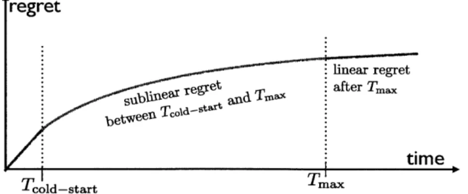
1.1 Regret Behavior of ITEM-ITEM-CF. Between Tcold-start and Tmax,N the al-gorithm achieves sublinear expected regret O(TT$1). After TmaxN the expected regret plateaus at a constant slope. The duration of the sublin-ear regime increases and the asymptotic linsublin-ear slope decreases with the

num ber of users. . . . 16

2.1 Observed Clustering of Users and Items (from BresLer et a[. (2014)). This is the densest subset of users (rows) and items (columns), where the darker spots indicate likes likes and the lighter spots indicate dislikes. One can see that the items and users can be grouped in relatively few types, where items of the same type tend to be liked by users of the same type. . . . . . 24

2.2

Jester

Doubling Dimensions . . . . 28

2.3 MovieLens Doubling Dimensions . . . . 28

3.1 Partition resulting from exploration in the previous epoch . . . . 32

3.2 During exploitation, items in Pk are recommended only when from a block when a user likes an item in the block . . . . 32

6.1 Expected Regret of ITEM-ITEM-CF, as proven in Theorems 5.1 and 5.2. . . . 63

(10)

(11)

Chapter 1 Introduction

M

1.1 Background

Whenever a business contains a large collection of items for sale, it is of interest to help customers find the items that are of most interest to them. Before the creation and widespread adoption of the Internet, this was done by trained store salesmen, who can

recommend items based on experience and the customers' revealed preferences.

After the creation of the Internet, this "recommendation system" has been largely taken off the hands of trained salesmen and is now largely handled by automated, statis-tically driven policies. For many companies, the efficacy of their recommendation systems stands at the core of their business, where Amazon and Netflix are particularly prominent

examples.

A natural and clever first idea in designing an automated recommendation system

is to use content specific data. In this spirit, one may use similar words in the title and book's cover, or a user's age and geographic location as inputs to recommendation heuristics. This type of recommendation system, where content-specific data is used, is called content filtering.

In contrast to content filtering, a technique called collaborative filtering (CF) provides recommendation in a content-agnostic way. CF works by exploiting patterns in general purchase or usage data. For instance, if 90% of users agree on two items (that is, 90% of users either like both items or dislike both items), a CF algorithm may recommend the second item after a user has expressed positive feedback for the first item.

The term collaborative filtering was coined in Goldberg et al. (1992), and this tech-nique is used in virtually all recommendation systems. There are two main paradigms in neighborhood-based collaborative filtering: the user-user paradigm and the item-item paradigm. To recommend to a user in the user-user paradigm, one first looks for similar users, and then recommends items liked by those similar users. In the item-item paradigm, in contrast, items similar to those liked by the user are found and subsequently

(12)

CHAPTER 1. INTRODUCTION

mended. Much empirical evidence exists that the item-item paradigm performs well in many cases (Linden et aL., 2003; Koren and Bell, 2011), and in this thesis, motivated to understand reasons behind this, we introduce a mathematical model and formally analyze the performance with respect to this model of a simple, intuitive algorithm (that we call

ITEM-ITEM-CF and describe in chapter 3) that follows the item-item paradigm.

*1.2

Organization of Thesis

The rest of this thesis is organized as follows. For the remainder of chapter 1 we formally introduce the model, give an informal overview of the main results, and discuss related works. In chapter 2 describe the assumptions that are made in light of theoretical lower bounds and empirical observations. In chapter 3 we describe our algorithm and in chapter 4 we prove the correctness of its main set of routines. In chapter 5 we put all the pieces together and give our main results pertaining to the performance of ITEM-ITEM-CF.

In chapter 6 we further discuss our results and list some future works.

*1.3

Model

Recommendation systems typically operate in an online setting, meaning that when a user logs into an virtual store (such as Amazon), a decision must be made immediately regarding which recommendations to make to that user. We model recommendation re-quests as follows: time is discrete and at each time step t a uniformly random user

Ut c {1,.., N} is chosen to be provided with a recommendation' It E I, where I is the universe of items. Furthermore, we impose the constraint that the recommendation algorithm may not recommend the same item to the same user twice2. For each time t, after being recommended item It, user Ut reveals the true preference Luj, for that item, which may be +1 (like) or -1 (dislike).

For each recommendation, the algorithm may either recommend an item that has been previously recommended to other users (in which case it has some information about whether or not at least one user likes the item) or recommend a new item from I.

For example, consider the toy example where we have N = 3 users. Suppose that

'This is equivalent to the model where each user is equipped with an independent exponential clock of the same rate, and a recommendation is requested by a user when his clock ticks.

2

The purpose of this work is to capture how well a recommendation algorithm can suggest new items to users rather the ones for which the users' preferences are already known. It is for this reason that we impose such a constraint. Of course, it also captures the setting where one is unlikely to buy the same book or watch the same movie twice.

(13)

we recommend item 1 to user 2, which then reveals that s/he likes it, i.e. L2,1 = 1. Then

the observed rating matrix Lobs and the (hidden) rating matrix L this time might be

+1 ?

L = +1 )Lobs (1

.

(1.1)

(-1 ?

Since each item is either liked (+1) or disliked (-1) by a given user, then each item is associated with a binary string of length N encoding likes/dislikes of the N users for it, and we call this binary string the type of i.

We are interested in the situation where there are many items, and will assume that

I is infinite. Therefore, from the N users' perspective, the population of items can be

represented as a distribution, denoted by p, over {-1, +1 }N. That is, when the algorithm wishes to recommend an item that hasn't yet been recommended, the item's type is drawn

3

from this distribution in an

i.i.d.

manner .

For instance, if

{

1/2 if x = [+1, +1, -1]T

p(x) = 12 fx[1,11],(1.2)

1/2 if x = [+1, -1, -1] T

and if the second recommendation was to user 3 was a new item (which turned out to be of type [+1, _1, - 1]T) then the rating matrices L and Lobs after that recommendation

would be

+1 +1 ? ?

L = +1 -1 ,Lobs = +1 ?

.

(1.3)

-1 -1 ? -1

Hence, we may think of p as a way of adding columns to the rating matrix when new items are recommended, where the new column is distributed according to p, and we will

refer to an item space by its distribution p.

* 1.4 Objectives of a Recommendation Algorithm

Given the setting above, we are interested in showing that an algorithm based on item-item collaborative filtering works well. A standard way to formally analyze online al-gorithms to is to look at its regret. The regret of a recommendation algorithm A is the

3

Note that such a model is quite general as we are imposing no constraints on how users like items, other than the restriction that preferences are binary (i.e. 1).

13 Sec. 1.4. Objectives of a Recommendation Algorithm

(14)

difference in reward relative to an all-knowing algorithm that makes no bad recommen-dations. In our case, the regret after T time steps can be formally defined as

T-N

R(T) N T 2 (1 - Lu,, (1.4)

t=1

as long as each user likes a positive fraction of items under p, which will always be the case. At time t the user Ut is desiring a recommendation, It is the recommended item, the variable Li is equal to +1 (resp. -1) if u likes (resp. dislikes) the item i, and N is the number of users4. The regret

R(T)

captures the expected number of bad recommendations per user after having made an average of T recommendations per user (hence the scaling by N in the definition of

R(T)).

Broadly, there are two main objectives in designing a successful recommendation algorithm:

" Cold-Start Performance: with no prior information, the algorithm should give re-liable recommendations as quickly as possible. The cold-start performance of an recommendation algorithm A is measured by

T cold-start -(A) = min m 1 T+F s.t. , T, F > 0,E[R(T + st , [ +A) - R(T)l ; 0.1(A+F),VA > 0

(1.5)

Intuitively this is the first time after which the algorithm's expected regret slope is bounded below 0.1. That is, from then on it can typically make a recommendation to a randomly chosen user and be wrong with probability at most 0.1. Whereas the choice of 0.1 is arbitrary, since we will assume that users tend to like only a small fraction of random items, one can think of the cold start time as the minimum time starting from when the algorithm can recommend significantly better than a random recommendation algorithm (which would make mostly bad recommendations). We want Tcod-start to be as small as possible, and in particular we will see that it need not grow with N.

" Improving Accuracy: the algorithm should give increasingly more reliable recom-mendations as it gains more information about the users and items, and this is captured by having sublinear expected regret. Ideally, we want E[R (T)] to be sublinear in T (i.e. a (T)) and as small as possible.

4

For notational simplicity we omit A on the notation of the regret and cold-start time, as the algorithm of interest wilL be clear from context.

(15)

e 1.5 Overview of Main Results

In this section we informally state our main results about the cold-start and improving ac-curacy of the algorithm ITEM-ITEM-CF (described in chapter 3), which is a simple, intuitive algorithm following the item-item paradigm.

Cold-Start Performance: We shall assume that each user likes at least v > 0 fraction of items. Then we have

(Achieving Cold-Start Time, Theorem 5.2) The algorithm ITEM-ITEM-CF achieves

Tcotd-start of 6(0).

One can relate this to a biased coin intuition, where we expect approximately 1/p coin flips until one gets a head. Similarly, in our case, since users like approximately v fraction of the items, it only takes (1Iv) for the user to find an item that is liked, and after this point the algorithm can recommend similar items. In light of the cold-start result, we would like to note a key asymmetry between item-item and user-user collaborative filtering. It is much easier to compare two items than it is to compare two users. Whereas it takes a long time to make many recommendations to two particular users, comparing two items can be done in parallel by sampling different users.

Improving Accuracy: Our first result states that unless some assumption is made on the items, no algorithm can perform well.

* (Lower Bound: Necessity of Structure, Proposition 2.1) With no structure on the item space, it is not possible for any algorithm to achieve sublinear regret for any period of time.

We will henceforth assume that the doubling dimension (which we define and motivate later, but the reader may simply think of it as a measure of complexity of the space of items) d of the item space is 0(1). Then

* (Sublinear Regime Regret Upper Bound, Theorem 5.1) the algorithm ITEM-ITEM-CF

achieves sublinear expected regret O(TTi2) until a certain time Tmax, after which the expected regret plateaus at a constant slope,

where Tmax increases with N and the slope decreases as a function with N, both of which illustrate the so-called collaborative gain5. Finally, we show that the

* (Lower Bound: Necessity of Linear Regime, Theorem 5.3) The asymptotic linear regime is unavoidable: every algorithm must have asymptotic regret

O(T).

sBy cotlaborative gain we mean the per-user performance improvement when we have many users, in comparison to the performance of only a single user using the system.

15

(16)

CHAPTER 1. INTRODUCTION

regret

linear regret reget after T mL betweeu Tco0da~t

time

Tcold-start Tma

Figure 1.1: Regret Behavior of ITEM-ITEM-CF. Between Tcotd-start and Tmax,N the algorithm d+1

achieves sublinear expected regret O(TmTT). After Tmax,N the expected regret plateaus at a constant slope. The duration of the sublinear regime increases and the asymptotic linear slope decreases with the number of users.

*1.6

Related Works

In this section we explore various related works. We begin by describing some relevant literature in multi-armed bandits, which deals with explore-exploit trade-offs similar to the ones a recommendation algorithm faces. We then, for completeness, describe matrix factorization methods of recommendation systems, which is another popular model of

recommendation system. We conclude by discussing other relevant works.

N

1.6.1 Multi-armed Bandits

The work on multi-armed bandits is also relevant to our problem. In the bandit setting, at each time t the user must choose which arm i

e

X (hence multi-armed) to pull in a slot machine (bandit). After pulling an arm i, the user receives a reward which is distributed according to an i.i.d. random variable with mean ri. The means {ri} are, however, unknown to the user, and hence the decision about which arm to pull depends on estimates of the means.

The goal of the user is to minimize the expected regret, which in this context the regret is defined as

R( T) = E ( *-r,,(1.6)

i

t=1

where It _{is the random variable denoting the arm pulled at time t and r*}_A _{supE-X r} is the supremum of expected reward of all arms. Hence, the expected regret measures

(17)

difference in expected rewards in comparison with an oracle algorithm that always pulls the arm with the highest expected reward.

The survey by Bubeck and Cesa-Bianchi (2012) thoroughly covers many other variants of multi-armed bandits, and points to Thompson (1933) as the earliest works in bandits. The multi-armed bandit work that is most relevant to us, however, is when X is a very large set, in which case we can interpret arms as item, and pulling an arm as recommending an item to a user. In this case of a large X (possibly uncountably infinite), however, some structure on X must be assumed for any algorithm to achieve nontrivial regret (otherwise one is left with a needle in a haystack scenario).

The works of Kleinberg et al. (2013) and Bubeck et al. (2011) assume structure on X and prove strong upper and lower bounds on the regret. They assume that the set X is endowed with some geometry: Kleinberg et al. (2013) assumes that the arms are endowed with a metric, and Bubeck et al. (2011) assumes that the arms have a dissimilarity function (which is not necessarily a metric). The expected rewards are then related to this geometry of the arms. In the former work, the difference in expected rewards is Lipschitz6 in the distance, and in the latter work the dissimilarity function constrains the slope of the reward around its maxima. In contrast, what is Lipschitz about our setting? Although slightly counter-intuitive since it involves many users, what is Lipschitz about our setting is the difference in reward when averaged among all users. That is

Eu[ILu,; - Lu,;I] ; 2 - yi,j, (1.7)

where yij is a distance between items, and will be defined in chapter 2.

d'+1

Those two aforementioned works show that the regret of their algorithm is O( T'+-2),

where d' is a weaker notion of the covering number of X, and is closely related to the doubling dimension (which we define later) in the case of metric. Our regret bound proven in Theorem 5.1 is of the same form, despite two important additional restrictions:

(i) in our case no repeat recommendations (i.e. pulling the same arm) can be made to the same user, and (ii) we do not have an oracle for distances between users and items, and instead we must estimate distances by making carefully chosen exploratory recommendations. Furthermore, unlike prior works, we quantify the cold-start problem.

6

That is, they assume that IE[rI - E[rj] ; C -d(i,j), where d is the distance metric between arms, and

C is a constant.

17 Sec. 1.6. ReLated Works

(18)

* 1.6.2 Matrix Factorization

Aside from neighborhood-based methods of collaborative filtering, matrix factorization is another branch of collaborative filtering that is widely used in practice. The winning team in the Netflix Challenge, for instance, used an algorithm based on matrix factorization, and due to its importance we will briefly cover some aspects of it here7_.

Using the language of recommendations, the set-up for matrix factorization is that we have a (possibly incomplete) n x m matrix L of ratings (where rows represent users and columns represent rows) that we would like to factor as L = AW, where A is n x r and W is r x m, and r is as small as possible. When L is complete, the singular value decomposition is known to provide the decomposition (cf. Ekstrand, Riedl, and Konstan (2011)). When L is incomplete, however, a popular approach in practice (cf. (Koren, Bell, and Volinsky, 2009)) is to use r = 1 and to find the decomposition by solving the regularized optimization problem

arg min ( Luj, - AUWi) + A (j|Au||2 +\|Wi|| (1.8)

A,W _(u,i)_observed

via, for instance, stochastic gradient descent (cf. (Zhang, 2004)). This, in effect, is looking for a sparse rank 1 factorization of L.

In many contexts, including that of recommendations, it also makes sense to want a nonnegative factorization. Intuitively, this enforces that we interpret each item as being composed of different attributes to various extents (rather than as a difference of attributes). Lee and Seung (2001) provided theoretical guarantees for fixed r, and Vavasis

(2009) then showed that this problem is NP-hard with r as a variable. The first provable

guarantee under nontrivial conditions came only later in Arora, Ge, Kannan, and Moitra (2012). They give an algorithm that runs in time that is polynomial in the m, n, and the inner rank, granted that L satisfies the so-called separability condition introduced

by Donoho and Stodden (2003)8.

In Section 2.4 we compare a rank notion to that of doubling dimension, which is structural assumption that we use here.

' As noted in Koren et aL (2009), matrix factorization techniques have some advantages over

neighborhood-based methods, such as the ease of combining it with content-specific data and of includ-ing implicit feedback.

8

Moitra (2014) surveys of all these and more results.

(19)

Sec. 1.6. Related Works

N

1.6.3 Other Related Works

It is possible that using the similarities between users, and not just between items as we do, is also useful. This has been studied theoretically in the user-user collaborative filtering framework in Brester, Chen, and Shah (2014), via bandits in a wide variety of settings (for instance Alon, Cesa-Bianchi, Gentile, Mannor, Mansour, and Shamir (2014); Slivkins (2014); Cesa-Bianchi, Gentile, and Zappella (2013)), with focus on benefits to the cold-start problem Gentile, Li, and Zappella (2014); Caron and Bhagat (2013), and in practice (Das, Datar, Garg, and Rajaram, 2007; Bellogin and Parapar, 2012). In this thesis, in order to capture the power of a purely item-item collaborative filtering algorithms, we purposefully avoid using any user-user similarities.

The works of Hazan, Kale, and Shalev-Shwartz (2012); Cesa-Bianchi and Shamir

(2013) on online learning and matrix completion are also of interest. In their case,

however, the matrix entries revealed are not chosen by the algorithm and hence there is no explore-exploit trade-off as we intend to analyze here.

Kleinberg and Sandler (2004) consider collaborative filtering under a mixture model in

the offline setting, and they make separation assumptions between the item types (called

genres in their paper). Dabeer (2013) proves guarantees, but their analysis considers a moving horizon approximation, and the number of users types and item types is finite and are both known. Biau, Cadre, and Rouviere (2010) prove asymptotic consistency guarantees on estimating the ratings of unrecommended items.

A latent source model of user types is used by Bresler et aL (2014) to give performance

guarantees for user-user collaborative filtering. The assumptions of user types and item types are closely related since K items types induce at most 2K user types and vice versa

(the K item types liked by a user fully identify the user's preferences, and there are at most 2K such choices). Since we study algorithms that cluster similar items together,

in this thesis we assume a latent structure of items. Unlike the standard mixture model with "gap" between mixture components (as assumed in all the above mentioned works), our setup does not have any such gap condition. In contrast, our algorithm works with effectively the most generic model, and we establish the performance of the algorithm based on a notion of dimensionality of the item space.

(20)

(21)

Chapter 2 Structure in Data

The main intuition behind all variants of collaborative filtering is that users and items can typically be clustered in a meaningful way even ignoring context specific data. Items, for example, can typically be grouped in a few different types that tend to be liked by the same users. It is with this intuition and empirical observation in mind that the two main paradigms in neighborhood-based collaborative filtering, user-user and item-item, operate. In the user-user paradigm, the algorithm first looks for similar users, and then recommends items liked by those similar users. In contrast, in the item-item paradigm items similar to those liked by the user are found and subsequently recommended. In this chapter we will develop the appropriate tools to exploit with structure in data. First, in Section 2.1 we show that without structural assumptions, the expected regret of any online algorithm is linear at all periods of time. In Section 2.2, we then develop our intuition for the structure present in data and define a distance between types of items. In Section 2.3 we then define the precise structural assumption that we will make: that the item space has finite doubling dimension. Finally, in Section 2.4 we give an example of how to relate the concepts of doubling dimension and low rank.

* 2.1 Need for Structure

As discussed, a good recommendation algorithm suggests items to users that are liked but have not been recommended to them before. To be able to suggest good/likable items to users, there are two basic requirements. First, at the heart of any recommendation algorithm, the basic premise is the ability to achieve "collaborative gain": in the item-item paradigm item-items similar to those liked by the user can be recommended, and in the user-user paradigm items liked by a similar user can be recommended. For any

any algorithm to achieve non-trivial "collaborative gain", it is necessary to impose some structural constraints on p. To that end, we first define what an online algorithm is, and then state the natural result stating that, in the worst case where y has little structure, 21

(22)

no online algorithm can do better than providing random recommendations.

Definition 2.1 (Online Recommendation Algorithm). A recommendation algorithm is called

an online recommendation algorithm if the recommendation at time t depends only on Ut, and

Us<,{

Us, Is, Lu,,I,, s}. That is, it has access only to the feedback received on

previous recommendations.

That is, an online recommendation algorithm has no access to knowing whether an item is liked or disliked by a particular user prior to recommending it.

Proposition 2.1 (Lower Bound). Under the uniform distribution p over {11, +1 }N, for all T > 1, the expected regret satisfies

E [R( T)] > T/2

for any online recommendation algorithm. Conversely, the algorithm that recommends a random item at each time step achieves R(T) = E [ T/21.

Proof We construct the desired item space by assigning p (v) = 2-N to each v E

{-1, 1 }N. That is, for every subset of users U C {0,..., N - 1} there exists an item type /u that is liked exactly by U and by no other users.

Now say that at time t we must make a recommendation to a user u, and let Mu be the set of items that have not yet been recommended to u. We will show that for each

i

e

Mu we have P (Luj =

+1

1 Ht) = 1/2, where H, is the history up to time t of users'

likes and dislikes. Let

Ri

be the set of users that have rated item i. Then, because the

N -

IR7i

other users may each like or dislike i, there are exactly 2N-7ZiI item types to

which i can belong. Furthermore, since half of those item types are liked by u and half are not liked by u and since all item types are equally likely (by our construction), we conclude that P (Lui = +11 Ht) = 2N12 = 1/2.

By the argument above, we have constructed an item space for which no algorithm

can do better than recommending wrong items in expectation half of the time. Now since

1 - Lu, = 2 when we make a bad recommendation at time t, we conclude that no algorithm can have expected regret lower than

ET

E![1 - Lus,] =

T

₁1/2 = T/2

over T recommendations.

Now consider the algorithm that recommends a random item at each time step. That is, at each time step t, we draw a new item It according to p, and recommend It to

Ut. Since p is uniform over {-1,+1}N, in particular the index corresponding to Ut is

uniform over {-1,+1} as well, and hence we have that P (Lt, = -1) = 1/2 for each

(23)

t. Since this is true for each time step, we conclude that this algorithm indeed achieves

E[R(T)] = T/2. M

Proposition 2.1 states that no online algorithm can have sublinear regret for any period of time unless some structural assumptions are made. Hence, to have any

collab-orative gain we need to capture the fact that items tend to come in clusters of similar

items. We will assume throughout that

(Al) the item space, represented by p, has doubling dimension at most d for a given d > 0,

where the doubling dimension is defined and motivated in Section 2.3.

Finally, if all users dislike all items or items are disliked by all users, then there is no way to recommend a likable item. Likewise, if users like too many items or some items are liked by too many users, then any regret benchmark becomes meaningless. To avoid such trivialities, we shall assume throughout that

(A2) each user likes a random item drawn from p with probability C [v, 2v], and

each item is liked by a fraction G [v, 2v] of the users, for a given v C (0, 1/4).

* 2.2 Item Types

To more formally describe item types and the conditions on p, let us first define a dis-tance between the item types. We shall endow the N-dimensional hamming space, i.e. {-1, +1 }N, with the following normalized 1 metric: for any two item types x, y E

{1, +1}N, define distance between them as

N 1

Yxy y(x, y) NT xk -Yk. (2.1)

k=1

When we write yij for items i,j, we mean the distance between their types, which is the fraction of users that disagrees on them.

One can plausibly go about capturing the empirical observation that items tend to belong to clusters that are liked by similar set of users is to assume that there are K different item types, and that the measure p assigns positive mass to only K strings in

{11+1 }N. Brester et al. (2014) do this, but where the users (instead of items) come in clusters. In addition, they assume that the types are well-separated (that is, yxy is lower bounded for each two different types x and y with positive mass). This allows for clustering perfectly with high probability, which in turn leads to a small regret.

23

(24)

CHAPTER 2. STRUCTURE IN DATA

U 1UU

Figure 2.1: Observed Clustering of Users and Items (from Bresler et aL. (2014)). This is the densest subset of users (rows) and items (columns), where the darker spots indicate likes likes and the lighter spots indicate dislikes. One can see that the items and users can be grouped in relatively few types, where items of the same type tend to be liked by users of the same type.

However, enforcing that the types are well-separated is counter-intuitive and not necessary for the following reason. If two types x and y are extremely close to each other, that should only make the problem easier and lead to a small regret, for if the algorithm mistakenly misclusters one type as the other, then the harm is small, as it will

lead to extremely few bad recommendations.

It turns out that we can exploit this intuition when the item space has sufficient structure, as captured by a certain notion of dimensionality.

M

2.3 Doubling Dimension

In order to capture this intuition that our mixture assumption should (i) give significant mass around item types and (ii) not have separation assumptions, we define a doubling dimension of p, and then further discuss its advantages. Let

B(x,

r) = {y e {-1, +1 }N

yx,y ; r} be the ball of radius r around x with respect to metric y'.

Definition 2.2. (Doubling Dimension) A distribution p on {-1, +1 }N is said to have dimension d if d is the least number such that for each x E {-l,+1}N with p(x) > 0 we have

p(B(x, 2r)) (

sup < 2 .(2.2) r>O p(3(x, r))

-Further, a measure that has finite doubling dimension is called a doubling measure.

'We omit the dependence of the bal on y throughout. 24

(25)

The above definition is a natural adaptation to probability measures on metric spaces of the well-known notion of doubling dimension for metric spaces (cf. (Heinonen, 2001; Har-Peled and Mendel, 2006; Dasgupta and Sinha, 2014)). As noted in, for instance Das-gupta and Sinha (2014), this is equivalent to enforcing that p(By(x, ar)) ad. p(By(x, r))

for any r > 0 and any x

E

{1,+1}N with p(x) > 0. For Euclidean spaces, the

dou-bling dimension coincides with the ambient dimension, which reinforces the intuition that metric spaces of

low

doubling dimension have properties of low dimensional Euclidean spaces.

Despite its simplicity, measures of low doubling dimension capture the observed clustering phenomena. Proposition 2.2 below, which follows directly from the definition, shows that a small doubling dimension ensures that the balls around any item type must have a significant mass.

Proposition 2.2. Let p be an item space for N users with doubling dimension d. Then

for any item type x E {-1, 1}N with p(x) > 0 we have

p(B (x, r)

)

;> r. (23)

Proof. Using the fact that B (x, 1) = {1,+1 }N for any x E {-1, +1 }N and the definition of doubling dimension we immediately get 1 = p (8 (x, 1)) 1

)

.p (B (x, r)) , which

proves the proposition. U

Doubling measures also induce many other nice properties on the item space, but let us first define an

c-net

for an item space.

Definition 2.1 (,-net). An c-net an item space p is a set C of items such that for a

random i drawn according to p, with probability 1 there exists c

E

C such that yi,c C. Furthermore, yi,j > -/2 for each two items i,

j

E C.

Proposition 2.3 below shows that, given an c-net of items, there can only be a small number of net items close to any given item.

Proposition 2.3. Let p be an item space for N users with doubling dimension d, let C

be an,-c-net for p, let

j

be an arbitrary item, let cj e C be such that yj,cj < -, and let Me; A p(B(cy,c)). Then, for each r e [c/2,112], there are at most meq

(4)d

(4r+5e d items in C within radius r of

j.

Proof By the doubling dimension of p we get

(

c;, r + c

)

5 p(B(c , c)). (r+504) = m. ( +5E/4 . (*)

25

(26)

We will now use this bound on p (13 (cp, r +

jc))

to show that we could pack at most

me₁(I)d (4r+5c)d items from C within r of j.

Since C is an c-net, each two items i,j

E

C are at least

c/2

apart, and hence the balls of radius c/4 around each i c C are disjoint. Say that there are K -

1C

₁

1

items C

within distance r of

j,

where Cj

A

{c E C I yc,j r}. Then we get

K -

( )

Zp (B(c, c/4)) = p(

U

8(c,E/4)) (B(cjr+5e/4)), (2.4)

ceC1 ccC;

where the first inequality is due to Proposition 2.2 and the

Last

inequality is due to

UcEccB(c,

c/4)

c

B(c, r + 5c/4). Using the bound from eq. (*) we arrive at

K<(4

)md

c r+5c/4 ) . (2.5)

as we wished.

To further illustrate and gain intuition for doubling dimension,

Let

us consider an example of doubling dimension of an item space.

Example 2.1. Consider an item space p over N users that assigns probability at least

w > 0 to K distinct item types with separation at least a > 0. Then, since p(B(x, a))

<

1, and p(B(x, a/2)) > w, we have that

d = max sup p(B<(x, r)) _<p2(x, a)) ( = Lo9₂1 /w. (2.6) xc{-1,+1}N r p(B(x, r/2)) p(B(X, a12)) t

Similarly, if we only know that there are at most K equally likely item types we can bound the doubling dimension as

d = max sup p(<3(x, r)) 1 lo92 K. (2.7)

x{-1,+1}N r

p(3(x,

r12)) - 1/K

With the example above in mind, we would like to emphasize that doubling dimension assumptions are strictly more general than the style of assumptions made in Brester et at. (2014) (finite K with separation assumptions) because (a) doubling measure require no separation assumptions (that is, two item types x and y that are arbitrarily close to each other can have positive mass) and (b) the number of types of positive mass is not bounded

by a finite K anymore, but instead can grow with the number of users.

(27)

Example 2.2. Consider an item space p such that it assigns probability 1/K to K item

types randomly uniformly drown from {-1, +1 }N. Then, for each two item types i, j we have that

P {yji [.4, .6} LP yZ [.4.6]) 5

(K)

exp(-O(N)), (2.8) where the first inequality is due to a union bound, and the second to a Chernoff bound. Hence, with high probability we get that

d>p(13(x, .7)) lo 2 1

d > pBx.)_= 10g2 - [092 K. (2.9)

- p(3(x, .35)) - 1/K

w.hp.

By Example 2.1 we also have that d < [o92(K), and hence we can conclude that with

high probability we have that d = lo92(K).

Finally, we would like to note that doubling dimension is not only a proof technique: it can be estimated from data and tends to be small in practice. To illustrate this point, we calculate the doubling dimension on the Jester Jokes Dataset2 and for the MovieLens

1M Dataset3. For the MovieLens dataset we consider the only movies that have been rated by at least 750 users (to ensure some density).

In both datasets we calculated the empirical doubling dimension di (that is, the smallest di such that p(B(i, 2r))

5

2dip(B(i, r)) for each r) around each item i. Under

a simple noise assumption, figs. 2.2 and 2.3 show that all the di tend to be small. The appendix A.2 describes the precise experiments.

* 2.4 Low Rank and Doubling Dimension

As mentioned in Section 1.6, a common assumption behind matrix factorization assump-tions is that the matrix has low rank. In this section we would like to draw a connection between rank properties of the rating matrix L and the doubling dimension of the item space induced by L. In particular, we will show that low doubling dimension is a weaker requirement than low right binary rank of L. To that end, we will first define what we mean by the item space induced by a rating matrix.

Definition 2.3. (Item Space induced by Rating Matrix) Let L be an N x M binary rating

2_{Goldberg et at.}

(2001), and data available on http://goldberg.berkeley.edu/jester-data/

3 RiedL and Konstan (1998), and data available on http://grouplens.org/datasets/movielens/

(28)

28 CHAPTER 2. STRUCTURE IN DATA 2 3 4 5 6 7 160 140 120 100 80 60 40 20 4 5 6 7 8

Figure 2.2: Jester Doubling Dimen- Figure 2.3: MovieLens Doubling

Di-sions mensions

matrix. Then the item space p induced by L is defined by

M

p(x) = 1Lj=x, for each xE {, +1IN. j=1

(2.10)

where Lj is the j'h column of L.

That is, the item space induced by a rating matrix assigns mass to item types according to the empirical frequency of the item type in L. For instance, the matrix

L =

(

-1 -1 +1 -1 +1 -1 -1 -1 +1 +1 +1 +1

)

(2.11)

has its induced distribution

PL(X) /2 /4 /4 if x if X if x (2.12) [ 1, +1, T [1, +1, -l]T.

The example below shows that there are rating matrices of high binary rank, but whose corresponding doubling dimension is constant (at most 2). Consider the N x N matrix LN whose

jth

column's first

j

entries are +1 and the remaining -1. That is, each of its columns different from its adjacent columns in exactly one entry. For instance, for

(29)

N = 4 we have

+1 +1 +1 +1

L4 1 +1 +1 (2.13)

-1 -1 +1 +1 -1 -1 -1 +1

The matrix LN clearly has rank N. However, the doubling dimension of its canonical item space is at most 2. We can see that because for each x and r

E

{0,..., N - 1}

L + r x r 1 + 2r (2.14)

which we can use to in turn conclude that

(B ( 2r 1 +4r

d < max maxlog2 (, < Log2( N) lo92 22 = 2. (2.15)

Hence, this shows that the doubling dimension of the induced item space can be substantially smaller than the rank of the rating matrix. Since the rank is a form of count of the number of item types, this again reinforces the fact that the number of types is not particularly important, but the geometric structure between them is.

29

(30)

(31)

Chapter 3 Description of Algorithm

In this chapter we describe the algorithm ITEM-ITEM-CF. The algorithm carries out a certain procedure over increasingly Larger epochs (blocks of time), where the epochs are denoted by T

E

N+. The epochs are of increasing time length, and in each epoch the

algorithm uses a careful balance of "Explore" and "Exploit" steps. Further, the algorithm begins with a period which is purely exploratory and aimed at the cold-start problem, and shortly after it the algorithm can already give meaningful recommendations to users. In the "Explore" steps of epoch T, a partition of items is produced that will be used

in the subsequent epoch. More precisely, in the epoch T, the "Explore" recommendations

construct a partition {P T+l)} of a set of items. In this partition we want that if two items

i

and

j

are in the same block P(r+), then yi <; Cr+1, where the Cr is defined below and

is the target precision at which the algorithm will construct the partition.

In the "Exploit" recommendations of epoch r, the partition {P T)} produced in the

previous epoch is used for providing recommendations to users. The algorithm follows a simple policy, where recommendations to a user u are made as follows: u samples a random item i from a random block P(T), and only if u likes i then the rest of p(T)

k' k

is recommended in future "exploit" steps. After all of P T) has been recommended, the

algorithm will use the future "exploit" steps for u to have u sample random items in random blocks until u likes another item

j

in P( T. The algorithm will then recommend the rest of P(T), and repeat the procedure until the epoch ends or it runs out of items, in which case it makes random recommendations. The pseudo-code of algorithm is as follows.

(32)

32 CHAPTER 3. DESCRIPTION OF ALGORITHM W. 2 , _P3

P

3

P

0

P 4e diameter ;e₁

for each block in {P} Figure 3.2: During exploitation, items in Pk are recommended only when from Figure 3.1: Partition resulting from ex- a block when a user likes an item in the ploration in the previous epoch block

ITEM-ITEM-CF(N)

1 Algorithm Parameters: IN 25d+18

v EN 25*8.630( 2d

+l1l)(d +

2)4-1-IN, C- =

ET = max

('

, N) -C, for T > 1 (target accuracy for epoch)

MT = 2 ax(35d,8) V (3 crerT ) Iln( C ), for T > 1 (number of items introduced in epoch)

DT = 2MT, for

r

> 1 (duration of epoch)

2 Cold-Start Epoch:

{P

}=

MAKE-PARTITION(M _1,E1, E1) 3 Subsequent Epochs: for T > 1 do for t = 1 to N -DT do u = random user

w.p. 1 - ET: exploit the partition {P(T} to give precise

recommendation to u (described in Section 3.1)

w.p. ET: give an explore recommendation to u to construct

the partition {P

}T+l)

(described in Section 3.2)

(33)

Sec. 3.1. Exploit 33

U 3.1 Exploit

Given the random user Ut at time t in some epoch T, ITEM-ITEM-CF provides exploit recommendations by using the partition {P(} in an intuitive way: whenever the user has liked an item, the algorithm recommends the rest of this item's block (consisting of hopefully similar items) to Ut in this user's subsequent exploit steps.

More formally, the exploit steps to Ut during epoch

r

have Ut sample a uniformly random item i from a uniformly random block P(T) that Ut hasn't yet sampled. If Ut likes i, then the algorithm recommends the remaining items of Pr in subsequent exploit steps to Ut. If there are no further items to recommend to Ut (i.e. all of p(T) has

been recommended, or Ut hasn't yet liked any items), then the algorithm has Ut sample another random item from a random block that Ut hasn't yet sampled. If there are no more blocks to be sampled (which we prove rarely happens), then the algorithm recommends an arbitrary item that has not yet been recommended to Ut.

N

3.2 Explore

Recall that during epoch T the goal of the explore recommendations is to create a partition

{P(T+l) } of items such that whenever ij E p+(T+) then yi :5 T+1 . We later prove that this can be done by executing the routine MAKE-PARTITION(MT+1, cT+1, CT+1) described

below, which at any point makes recommendations to a randomly chosen user. Hence, given the random user making the recommendation, ITEM-ITEM-CF provides explore rec-ommendations in whatever order MAKE-PARTITION would have recommended (had it been run sequentially).

For instance, suppose that time t is the first in some epoch T. We might have that

times t + 5 and t + 30 are the first two explore recommendations of the epoch, then for those two recommendations the algorithm makes whatever the first two recommendations would have been in MAKE-PARTITION. If the execution of MAKE-PARTITION has finished, the algorithm resorts to an exploit recommendation instead.

We now describe MAKE-PARTITION. This routine has two main steps:

* (create c-net): finds a set of items C such that with high probability for an item

i

drawn from the item space there is an item

j

E C with yi] <

"r+1-* (create partition): using C as a starting point, the algorithm creates a partition {Pk}

of items such that with high probability all items in the same block are ET+1 close

(34)

We now describe MAKE-PARTITION in more detail, and the pseudocode is below (where the routines SIMILAR and GET-NET are described later). First it finds a net for the item space (using the subroutine GET-NET), and then partitions a set of items using the net as the starting point. For each of the M items sampled, MAKE-PARTITION finds an item

i

e

C that is similar to the item

j

sampled, and assigns

j

to the partition block Pi of items similar to i (in case there is more than one such item i, the algorithm breaks ties at random). Finally, the algorithm breaks up large blocks into blocks of size on the order of

1/c. This guarantees that there will be many blocks in the partition, which is important

in Lemma 5.1 in ensuring a good cold-start performance.

MAKE-PARTITION(M, c, 6)

1 C = GET-N ET(C/2, 5/2)

2 M = M randomly drawn items from item space 3 for each

i

e C

4 do let Pi = 0

5 for each

j

c M

6 do Sj = {i

I

sIMILAR(i, j, 0.6,, returns TRUE)} 7 if IS;1 > 0 then

8 Pi = Pi U

j,

for i chosen u.r. from S

9 if IPil > 1/c for any i, partition Pi into blocks of size at most

10 return {Pi}

It is crucial that blocks in the partition are not too small. This is important because we would like the reward for exploration to be large when a user finds a likable item (reward in the sense of many new items to recommend). Although the algorithm does not explicitly ensure that the blocks are not too small (as it did in ensuring the blocks are not too large) it comes as a byproduct of-a property proven in Proposition 2.3, which shows that there are not many items in the net very close to any given item

j.

The subroutine SIMILAR is used throughout MAKE-PARTITION, and it aims at deciding whether most users agree on two items i and ] (that is, whether most users like or dislike

i

and

j

together). It does so by sampling many random users and estimating the fraction that disagree on the two items.

(35)

SIMILAR(i, j, -, 6)

1 gc,6

= [630

d+ln

(-!)

2 for n = 1 to q,,

3 do sample a uniformly random user u 4 let Xu = I{Luj * Luj }

I f sampted u Xu > 0.9c then

6 return FALSE

7 If Zsampted u Xu <

0.9c

then

8 return TRUE

The subroutine GET-NET below is a natural greedy procedure for obtaining an E-net.

Given parameters

E

and 6, it finds a set of items C that is an

E-net

for p with probability at Least 1 - 6 (proven in the appendix). It does so by keeping a set of items C and whenever it samples an item i that currently has no similar item in C, it adds i to C. GET-NET(C, 5)

1 C = 0

2 MAX-SIZE = (4/c)", MAX-WAIT = ($)d In (2-MAsIzE ' = 61(4- MAX-WAIT MAX-SIZE 3 COUNT = 0

4 while COUNT < MAX-WAIT and JCI < MAX-SIZE 5 do draw item i from p

6 if SIMILAR(ij, c, 6') for any

j

E C then

7 COUNT COUNT +1 8 else C=CUi 9 COUNT= 0 10 return C 35 Sec. 3.2. Explore

(36)

(37)

Chapter 4 Correctness of Explore

In this chapter we will prove that with high probability the procedure MAKE-PARTITION

indeed produces a partition of similar items during each epoch. In Section 4.1 we prove that SIMILAR succeeds in deciding whether two items are close to each other. In Section 4.2 we prove that the procedure GET-NET succeeds in finding a set of items that is an

c-net

for p. We then put all the pieces together and prove that MAKE-PARTITION, the routine at which the explore recommendations are aimed at completing, succeeds in creating a partition of similar items. Finally, in Section 4.3 we prove that with high probability during any given epoch there will be enough explore recommendations.

U

4.1 Guarantees for

SIMILAR

The procedure SIMILAR (which we restate below for convenience) is used throughout GET-NET and MAKE-PARTITION, and it is aimed at testing whether two items are approximately c-close to each other.

SIMILAR(, j, c, 6)

1 qc,6 = [6304-1 Ln (1)]

2 for n = 1 to,

3 do sample a uniformly random user u

4 Xu = I{Loi * Luj}

5 if i-, Esampled u X, > 0.9c then

6 return FALSE

7 If I Tsampted u Xu < 0.9c then

8 return TRUE

The Lemma below shows that given two items i and j, SIMILAR indeed succeeds in telling the items are similar when yij <

0.8c,

and that the items are not similar when

Yij >

Collaborative filtering with low regret