Combinatorial Optimization Problems with Concave Costs
by
Dan Stratila
MASSACHUSETTS
INSTITUTEDiploma, Computer Science,
2002
FEB 2 7
2
009
Moldova State University
L BRARIES
Submitted to the Sloan School of Management
in partial fulfillment of the requirements for the degree of
DOCTOR OF PHILOSOPHYIN OPERATIONS RESEARCH
at the
MASSACHUSETTS INSTITUTE OF TECHNOLOGY
February 2009
@
Massachusetts Institute of Technology 2009.
All rights reserved.
A u th o r ...
.
..
...
Sloan
4oo
oo anagement
September 12, 2008
Certified by ...
Accepted by
...
Co-Thomas L. Magnanti
Institute Professor
Thesis Supervisor
Dimitris J. Bertsimas
Professor of Operations Research
-director, Operations Research Center
Combinatorial Optimization Problems with Concave Costs
by
Dan Stratila
Submitted to the Sloan School of Management on September 12, 2008 in partial fulfillment
of the requirements for the degree of Doctor of Philosophy in Operations Research
Abstract
In the first part, we study the problem of minimizing a separable concave function over a polyhedron. We assume the concave functions are nonnegative nondecreasing on R+, and the polyhedron is in RI' (these assumptions can be relaxed further under suitable technical conditions). We show how to approximate this problem to 1 + precision in optimal value by a piecewise linear minimization problem so that the number of resulting pieces is polynomial in the input size of the original problem and linear in 1/c. For several concave cost problems, the resulting piecewise linear problem can be reformulated as a classical combinatorial optimization problem. As a result of our bound, a variety of polynomial-time heuristics, approximation algorithms, and exact algorithms for classical combinatorial optimization problems immediately yield polynomial-time heuristics, approximation algorithms, and fully polynomial-time approximation schemes for the corresponding concave cost problems. For example, we obtain a new approximation algorithm for concave cost facility location, and a new heuristic for concave cost multicommodity flow.
In the second part, we study several concave cost problems and the corresponding com-binatorial optimization problems. We develop an algorithm design technique that yields a strongly polynomial primal-dual algorithm for a concave cost problem whenever such an algorithm exists for the corresponding combinatorial optimization problem. Our technique preserves constant-factor approximation ratios as well as ratios that depend only on cer-tain problem parameters, and exact algorithms yield exact algorithms. For example, we obtain new approximation algorithms for concave cost facility location and concave cost joint replenishment, and a new exact algorithm for concave cost lot-sizing.
In the third part, we study a real-time optimization problem arising in the operations of a leading internet retailer. The problem involves the assignment of orders that arrive via the retailer's website to the retailer's warehouses. We model it as a concave cost facility location problem, and employ existing primal-dual algorithms and approximations of concave cost functions to solve it. On past data, we obtain solutions on average within 1.5% of optimality, with running times of less than 100ms per problem.
Thesis Supervisor: Thomas L. Magnanti Title: Institute Professor
Acknowledgments
I am grateful to my advisor, Tom Magnanti, for his support and guidance over the years. Thanks to him, I have learned a lot about research and teaching during my graduate school years. Tom's encouragement at every step of the way has been invaluable, and I very much appreciated his willingness to experiment and let me pursue my own ideas. Inevitably, this meant that I have also learned a lot from my mistakes while being his student.
I would like to thank the other members of my committee, Michel Goemans, Retsef Levi, and David Simchi-Levi for their insightful comments and ideas on the research in this thesis and beyond. I am grateful to Jim Orlin for his advice and guidance ever since I entered graduate school. I learned in many ways from Jim-from refereeing papers to being a teaching assistant. I thank Russell Allgor for his input and support of my computational research. I would also like to thank Dimitris Bertsimas and Georgia Perakis for their help and advice.
I was fortunate to have started at MIT at a time when Martin Skutella was a visiting professor and was teaching the basic integer programming and combinatorial optimization course-I have never learned more per unit of time in any other class. In subsequent years, Michel Goemans' advanced graduate classes on combinatorial optimization and polytopes have been a very enriching experience.
Thanks to my fellow ORC students, and especially Raghavendran Sivaraman, Pranava Goundan, and Ping Xu, as well as my officemates over the years, Alexandre Belloni, Shobhit Gupta, Kwong Meng Teo, and Pavithra Harsha. Many thanks to Alex Andoni and Dumitru Daniliuc. I am very grateful to Carol Meyers, among other things for her unbounded patience and always very positive attitude.
My thanks go to my host family at MIT, Ellen and Richard Lacroix. Finally, I would like to thank my parents and grandparents.
This research was supported in part by the Air Force Office of Scientific Research, Amazon.com, and the Singapore-MIT Alliance.
Contents
1 Introduction 13
1.1 Concave Cost Facility Location ... ... . 14
1.1.1 Literature Review ... .. . . . . 17
1.2 Concave Cost Multicommodity Flow . ... ... . 19
1.2.1 Literature Review ... .. . . . . 21
1.3 Concave Cost Lot-Sizing ... . . . . . . 23
1.3.1 Literature Review ... .. . . . . 25
1.4 Concave Cost Joint Replenishment . ... ... 26
1.4.1 Literature Review ... ... . 28
2 Piecewise-Linear Approximations 29 2.1 Literature Review ... ... ... .. .. 30
2.1.1 Our Results ... ... .. 31
2.2 General Feasible Sets ... ... .. 32
2.2.1 A Lower bound on the Number of Pieces . ... 35
2.2.2 Extensions . ... ... .. 37
2.3 Polyhedral Feasible Sets ... ... . 38
2.3.1 Representing the Piecewise Linear Functions . ... 39
2.4 Multicommodity Flows ... ... . . 40 2.4.1 Computational Results ... ... 41 2.5 Facility Location ... .... .... .... . 43 3 Primal-Dual Algorithms 47 3.1 Literature Review ... ... 48 3.1.1 Our Contribution ... ... . 49 3.2 Preliminaries ... ... 50 3.2.1 A Primal-Dual Algorithm ... ... 51 3.3 The Technique ... .. ... 53
3.3.1 Analysis of a Single Facility ... .... 55
3.3.2 Other Rules for Changing the Dual Variables . ... 61
3.3.3 Analysis of Multiple Facilities ... ... 62
3.5 Joint Replenishment with Concave Ordering Costs . ... . . . . 69
4 Single Order Assignment 75
4.1 The Single Order Assignment Problem ... .. 76
4.2 Concave Cost Models . . . ... ... 78
4.3 Computational Results ... ... . 79
List of Figures
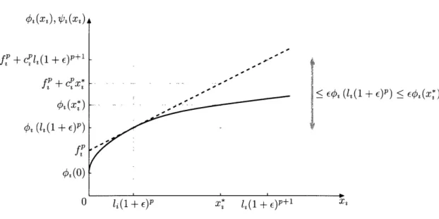
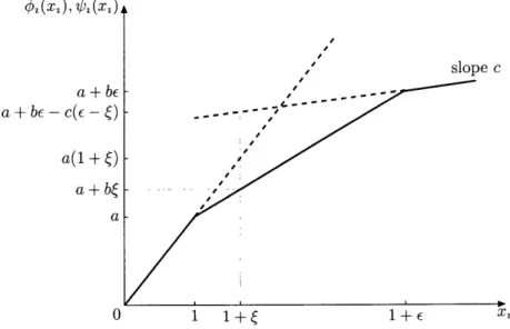
2-1 Illustration of the proof of Lemma 7. Observe that the height of any point inside the box with the bold lower left and upper right corners exceeds the height of the box's lower left corner by at most a factor of E. . ... 34 2-2 Illustration of the proof of Theorem 1. . ... . . 35 3-1 Illustration of the proof of Lemma 12. . ... . . . . 56 3-2 Illustration of the proof of Lemma 12. Here U = {1, 2} and C = {3, 4}. The
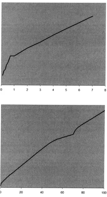
gray arrows show how pi(t) change as t increases. . ... . 60 4-1 A sample cost function experienced by the retailer for a given shipping
method from a given fulfillment center to a given customer. The horizon-tal scale represents the weight in lbs. The vertical scale represents the cost, however the units are omitted to exclude retailer confidential information. 77
List of Tables
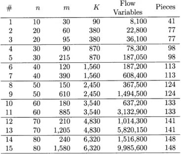
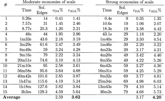
2.1 Network sizes. The column "Pieces" indicates the number of pieces in each piecewise linear function resulting from the approximation. . ... 43 2.2 Computational results. The values in column "Sol. Edges" represent the
number of edges with positive flow in the obtained solutions. ... . 44 4.1 Computational results for the single-order assignment problem. . ... 80
Chapter 1
Introduction
In this thesis, we study problems that can be written as the minimization of a concave cost function over a polyhedron. Such problems arise frequently in fields such as transportation, logistics, telecommunications, and supply chain management. In a typical application, the polyhedral ground set is due to network structure, capacity requirements, and other constraints, while the concave costs are due to economies of scale, volume discounts, and other practical factors [see e.g. GP90]. In particular, we obtain new results for concave cost facility location, concave cost multicommodity flow, concave cost lot-sizing, and concave cost joint replenishment.
We are interested in two types of solution methods. First, we seek algorithms with prov-able theoretical properties-for example, exact time algorithms, polynomial-time approximation schemes, and approximaiton algorithms. Second, we are interested in algorithms that do not have theoretical properties or have properties that are unattractive in practice, but that nonetheless can be shown to perform well in computational experiments to an extent that makes them promising candidates for practical implementation.
The methods for solving separable concave cost minimization problems with polyhedral feasible sets can be classified into two broad categories. The methods in the first category rely on piecewise-linear approximations. After one approximates the concave cost functions by piecewise-linear functions, the resulting problem can be written as a mixed-integer pro-gram, and often this mixed-integer program represents a classical combinatorial optimiza-tion problem. Therefore, a variety of methods from integer programming and combinatorial optimization become immediately available for solving the concave cost problem.
In order for this approach to be successful, we must be able to approximate the concave cost problem by a single piecewise-linear problem that has few pieces and at the same time provides a good approximation to the original problem in terms of optimal cost. Chapter 2 focuses on devising methods for approximating concave functions and on bounding the resulting number of pieces.
The second broad category for solving concave cost problems consists of algorithms de-signed to operate directly on concave cost problems. In this category we include algorithms that perform piecewise-linear approximations iteratively as part of their computations.
Di-rect algorithms can avoid the quality of approximation/number of pieces tradeoff inherent in any linear approach, and can overcome several other limitations of the piecewise-linear approach as well.
However, direct algorithms must be designed with concave cost problems in mind, often on an individual problem basis. For this reason, there are significantly fewer algorithms for concave cost problems than for the corresponding (or comparable) classical combinatorial optimization problems. In Chapter 3 of this thesis, we develop a technique for obtaining primal-dual algorithms for concave cost problems based on such algorithms for combinatorial optimization problems. First we develop several general insights, and then apply them to three specific problems.
In the remainder of this chapter, we introduce the specific problems studied in this thesis, describe their basic properties, and review the literature on them. Section 1.1 describes the concave cost facility location problem, and Section 1.2 the concave cost multicommodity flow problem. Then we introduce two inventory problems-concave cost lot-sizing in Section 1.3 and concave cost joint replenishment in Section 1.4.
In Chapter 2 we develop new methods and bounds for piecewise-linear approximations of concave functions. In Section 2.1 we conduct a literature reivew, and in Sections 2.2 and 2.3 we develop a general technique for concave cost problems. In Sections 2.4 and 2.5 we apply the technique to concave cost multicommodity flow and concave cost facility location. In Chapter 3 we develop a technique for obtaining primal-dual algorithms for concave cost problems. Section 3.1 contains a literature review, Section 3.2 introduces some pre-liminary notions, Section 3.3 develops our technique on the basis of facility location, and Sections 3.4 and 3.5 apply it to lot-sizing and joint replenishment.
In Chapter 4 we develop a computational solution method for an order assignment problem encountered at a large internet retailer. We describe the problem in Section 4.1, model it as a concave cost facility location problem in Section 4.2, and present computational results in Section 4.3.
1.1
Concave Cost Facility Location
Let [n] = {1,..., n}. In the concave cost facility location problem, there are m customers
and n facilities. Each customer i has a demand di > 0, and needs to be connected to a facility to satisfy this demand. Connecting a customer i to a facility j incurs a connection cost cijdi; we assume the connection costs are nonnegative and satisfy the metric inequality. Let xij = 1 if customer i is connected to facility j, and xij = 0 otherwise. Then the total demand satisfied by facility j is E 1 , dsxi1. Each facility j has an associated concave cost
function Oj : R+ -* R+, and we assume the functions qj are nondecreasing. We also assume without loss of generality that Oj(0) = 0 for j c [n]. At each facility j we incur a facility cost of Oj (1' dicij). The goal of the problem is to assign each customer to a facility, while minimizing the total connection and facility cost.
1.1. CONCAVE COST FACILITY LOCATION 15
The concave cost facility location problem can be formulated as a mathematical program:
n m n
Z. 1 = min
>
j ( dixij + cijdixzj, (1.1a)j=1 z=1 i=1 j=1
s.t. E x 3 = 1, i [], (1.1b)
3=1
xij > O, i E [m],j j [n]. (1.1c)
Given a solution x to this problem, we will refer to its cost as Zi.i(x). (Sometimes the problem is formulated to include the constraints xij E {0, 1}. Since we are minimizing a concave function over a polyhedron, there is always an optimal solution at an extreme point of the polyhedron [e.g. Bau58], and an extreme point solution automatically satisfies these constraints.)
The classical facility location problem is the special case when the cost Oj at each facility has the form
fj, (j> 0, (1.2)
J(6)= (0, j = 0.
Such a cost function is also known in the literature as a fixed charge. We will sometimes refer to the classical facility location problem as the fixed-charge facility location problem. The classical facility location can be formulated as a mixed-integer program. To do so, introduce a binary variable yj for each facility j, with the interpretation that y, = 1 if j is open, and yj = 0 otherwise:
n m n
min E fjyj +
>
E c,3dixij, (1.3a)j=1 i=1 j=1 n s.t. xij = 1, i E
[m],
(1.3b) j=1 0 < X2z < yj, i E [m],j E [n], (1.3c) yj E {0, 1}, i E [m],j E [n]. (1.3d)Next, we describe two basic properties of the concave facility location problem. A concave function defined on [0, +oo) is continuous everywhere except at 0. Next, we consider concave functions that, in addition, are piecewise-linear everywhere except at 0.
Lemma 1. Consider the concave cost facility location problem. Let the cost functions Oj
be piecewise-linear everywhere except at 0, and consist of P pieces each. Then the problem can be reduced to the classical facility location problem with P times as many facilities. Proof. We start with the concave cost problem. Since a piecewise-linear concave function
consisting of P pieces can be expressed as the minimum of P affine functions, we can write
rmin{fjp + sjpj : p E [P]}, j > 0,
0.()
= 0(1.4)
0, 3 = 0.
Substituting this equation into problem (1.1) and reformulating, we obtain:
n P m n P
min
E
E fjpyjp +S
E(cij + s3p)dzxijp, (1.5a)j=1 p=1 i=1 j=1 p=l n P s.t. E ijp = 1, i E [m], (1.5b) j=1 p=l 0 Xijp < yjp, i E [m],j E [n],p E [P], (1.5c) yjp E {0, 1}, i [m], j E [n],p E [P]. (1.5d) This mixed-integer program has the structure of a classical facility location problem with
Pn facilities and m customers. Every piece p in the cost function Cj of every facility j in
the original concave cost problem corresponds to a facility {j, p} in the new problem. The new facility has opening cost fjp. The customer set is the same, and the connection cost from facility {j, p} to customer i is cij + sjp.
The new facility costs fjp and the new connection costs cij + sjp are nonnegative. Since the original connection costs c,, satisfy the metric inequality, so do the new connection costs
cij + sjp. Therefore, formulation (1.5) is a classical facility location problem. 1O
This reduction is well known in the literature, and dates back to the 1960-s [e.g. FLR66]. More recently this reduction has been employed for example by Hajiaghayi et al. [HMM03] and Mahdian et al. [MYZO6].
When the concave functions are piecewise-linear and the pieces are given explicitly in the input, the size of the resulting classical facility location problem is polynomial in the size of the original concave cost problem. Therefore, a polynomial-time approximation algorithm for the classical facility location problem immediately yields a polynomial-time approximation algorithm for the concave cost facility location problem. The same is true for polynomial-time heuristics.
However, this reduction does not result in a polynomially sized instance when the func-tions are given by an oracle, or are nonlinear and given algebraically. And computationally, when each function consists of a large number of pieces, the resulting algorithms can be very inefficient.
Next, we show how to use the demand structure to perform this reduction for general concave functions. Let X =
{
E is di : S C [m], S#
0}.
Since we are minimizing a concave function over a polyhedron, the concave cost problem always has an optimal solution x* such that for every facility j, the total demand of all customers assigned to j is in X, i.e.1.1. CONCAVE COST FACILITY LOCATION
Lemma 2. The concave cost facility location problem can be reduced to the classical facility
location problem with IX
I
times as many facilities.Proof. Take concave cost problem (1.1). We approximate each concave function Oj by a
concave function 4j that is piecewise-linear everywhere except at 0, consists of IXI pieces,
and is such that 0j( j) = 4j(j) for (3 E X, and C j(j) > Oj((j) for (j > 0. This can be
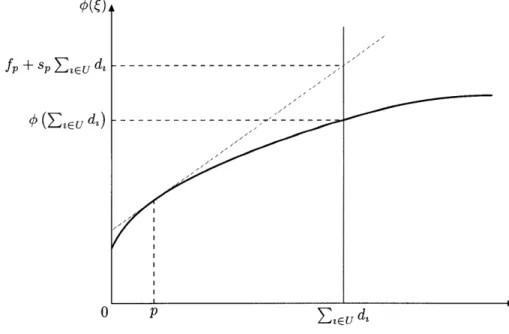
done, for example, by taking a supergradient fjp + sjpj to Oj at each point p
c
X, andthen letting bj( j) = min{fjp + sjpj : p E X} for (j > 0, and j(O) = 0.
Now consider the concave cost problem obtained from problem (1.1) by replacing the functions ¢. with 4j:
n m n
Z1.6 = min 1 dixij + E cijdixij, (1.6a)
j=1 i=1 i=1 j=1
n
s.t. Ex i = 1, i E [m], (1.6b)
j=1
x 3 2 0, i [m],j
c
[n]. (1.6c)Let x* be an optimal solution to problem (1.1) with Em, dix* X for j [n]. Since j( 3) = OJ(Qj) for j E X, we have Zl*.6 < Zi.6(x*) = Zi.i(X*) = Z".1 . Conversely, let y* be an optimal solution to problem (1.6). Since Oj( ) > Oj( j) for j > 0, we have Z. 6 = Zi.6(y*) > Zi.i(y*) 2 Z.1. Therefore, Z1*6 = Z1.1.
By Lemma 1, problem (1.6) can be reduced to the classical facility location problem
with IXI times as many facilities. O
When the concave cost facility location has uniform demands, i.e. dl = d2 = din, we have IXI = m, and this reduction yields a classical facility location problem with m times as many facilities. Therefore, in this case too, a polynomial-time approximation algorithm or heuristic for the classical facility location problem immediately yields a polynomial-time approximation algorithm or heuristic for the concave cost facility location problem.
In general, IXI is exponentially sized, and this approach does not lead to polynomial-time algorithms for the concave cost problem.
1.1.1 Literature Review
The classical facility location problem is one of the fundamental problems in operations research, and has been studied since at least the 1960's [e.g. KH63, Sto63, Ba166]. The reference book edited by Mirchandani and Francis [MF90] introduces and reviews the liter-ature for many problems, including the uncapacitated facility location problem [CNW90]. Since in this thesis, our main contributions to facility location problems are in the area of approximation algorithms, we next provide a survey of previous approximation algorithms for classical facility location.
The first approximation algorithm for this problem was proposed by Hochbaum [Hoc82] and applied to the case when the connection costs cij did not necessarily satisfy the metric inequality. This algorithm achieved an approximation ratio of O(log n). Shmoys et al. [SETA97] gave the first constant-factor approximation algorithm for this problem.
More recently, Jain et al. introduced 1.861 and 1.61 primal-dual approximation algo-rithms [JMM+03]. Sviridenko [Svi02] obtained a 1.582 approximation algorithm based on LP rounding. Mahdian et al [MYZO6] developed a 1.52 approximation algorithm that com-bines a primal-dual stage with a scaling stage. Currently, the best known ratio is 1.4991, achieved by an algorithm that employs a combination of LP rounding and primal-dual techniques, due to Byrka [Byr07].
Concerning the complexity of approximation, the problem where the connection costs do not necessarily obey the metric inequality has the set cover problem as a special case, and therefore is not approximable to within a constant factor unless P=NP [e.g. RS97]. The problem with metric costs is not approximable to within a factor of 1.46 unless NP C
DTIME (no(loglogn)) [GK99].
A central feature of location models is the economies of scale that can be achieved by connecting multiple customers to the same facility. The classical facility location problem models this effect by assigning to each facility a fixed-charge cost, as defined in equation (1.2). As one of the simplest forms of concave functions, fixed-charge costs enable the model to capture the essential tradeoff between opening many facilities in order to decrease the connection costs and opening few facilities to decrease the facility costs. The concave cost facility location problem generalizes this model by assigning to each facility a general concave cost function, and as such captures a much wider variety of phenomena than is possible with fixed costs alone.
The concave cost facility location problem has also been studied since at least the 1960's [e.g. KH63, FLR66]. Since it contains classical facility location as a special case, the pre-viously mentioned lower bounds on approximability hold for this problem-the nonmetric version cannot be approximated within a constant factor unless P=NP, and the metric prob-lem cannot be approximated to within a factor of 1.46 unless NP C DTIME (no(log log n)).
However, the results in the area of approximation algorithms are significantly more limited than for the classical problem. To the best of our knowledge, previously the only constant factor approximation algorithm was obtained by Mahdian and Pal [MP03]. They developed a 3 + c approximation algorithm based on local search. Their analysis is based in part on the analysis of the local search algorithm by Charikar and Guha [CG99, CG05]. When the concave cost facility location problem has uniform demands, a wider variety of results become available. Hajiaghayi et al. [HMM03] obtained a 1.861 approximation algorithm. A number of results become available due to the fact that, as described in Lemma 2, concave cost facility location with uniform demands can be reduced in polynomial size to classical facility location. For example, Hajiaghayi et al. [HMM03] and Mahdian et al. [MYZO6] described a 1.52 approximation algorithm.
After completion of this research, we learned of the independent research of Romeijn et al. [RSSZ07]. They develop 1.61 and 1.52 approximation algorithms for concave cost
1.2. CONCAVE COST MULTICOMMODITY FLOW
facility location, by considering the corresponding algorithms for classical facility location [JMM+03, MYZO6] through a greedy perspective. Since our analysis in Chapter 3 uses a primal-dual perspective, establishing a connection between the research of Romeijn et al. and ours is an interesting question.
1.2
Concave Cost Multicommodity Flow
The concave cost multicommodity flow problem is defined on an undirected network (V, E) with node set V and edge set E; we let n = IVI and m = IEl. On this network, there
flow K commodities, and each commodity k has sources and sinks, which are given via a demand and supply vector b , i e V. A coefficient bk > 0 indicates that node i is a source of commodity k, and the supply is bk; b < 0 indicates that i is a sink of commodity k and the demand is -b k. We assume that the supply and demand are balanced, that is E
2
v bt = 0 for k e [K], and that the network is connected, i.e. it contains a path between any twonodes.
Each edge {i,
j}
E has an associated concave cost function Oi3 : R+ -- R+, and+ we assume that Oij are nondecreasing. Without loss of generality, we let Oij(0) = 0 for{i,j} E E. For an edge {i,j} E E, let xk indicate the flow of commodity k from i to
j,
andxji the flow in the opposite direction. Then the total cost of routing flow on edge {i,j} is EK I(=1i j + Xk )). The goal is to route the flow of each commodity so as to satisfy the
demand at all sinks, while minimizing total routing cost.
A mathematical programming formulation for this problem is given by:
(K
min E ij ( + xji) , (1.7a)
{t'j}GE (k=1
s.t. = b , k b- i V, k e[K], (1.7b)
{i,j}EE {j,i}EE
S Ix > , {i,j} E E, kEG [K]. (1.7c)
Let ij = xK (2X + xk) be the total flow on an edge {i,j} E E. The fixed-charge multicommodity flow problem is the special case when the edge cost functions have the
form:
= fij + sjij, 3
> O, (1.8)
S
= o(1.8)
Similarly to the functions (1.2), these functions are often referred to as fixed-charge functions
in the literature. Let Bk = Zi:b>0 k b be the total supply of commodity k, and B =
~E
1Bk be the total supply of all commodities.The fixed-charge multicommodity flow problem can be formulated as a mixed integer program: min E fijyij {i,j}EE s.t.
5
A -{2,31}E KE
E
{i,j}EE k=1 {j,i}EE 0< za,xi < BkYij , Yi E {0, 1}, iE V,k E [K], {i,j} E E,k E [K], {i,j} C E. (1.9a) (1.9b) (1.9c) (1.9d) In this setting, for each edge {i,j},
the coefficient fij can be interpreted as its installation cost, and cij as the per-unit cost of routing flow on the edge once installed.The fixed-charge multicommodity flow problem when each commodity has only one source or one sink can be reduced to the case when each commodity has one source and one sink, by creating a new commodity for each source-sink pair. The latter problem is also called uncapacitated network design in the literature [e.g. BMW89]. Our theoretical results in Chapter 2 will apply to concave cost multicommodity flows with any demand pattern, while our computational results in Section 2.4 will focus on concave cost multicommodity flow where each commodity has one source and one sink.
As in the case of facility location, when the concave cost functions are piecewise linear everywhere except at 0 and consist of P pieces each, the concave cost multicommodity flow problem reduces to a fixed-charge multicommodity flow problem with P times as many edges. Let the concave functions be:
) min{fijp + sjjpij : p E [P]}, ij > 0,
0, ~iJ = 0.
(1.10)
Substituting these expressions into problem (1.1) and reformulating, we obtain: K min fipyijp + Stp(kP + {i,j,p}EE {i,j,p}EE k=1 s.t. A A = b k E 2 -- E zjp i {i,j,p}EE {j,z,p}EE 0 < xk, xk < Bkyijp, y-Jp E { j1 z Yijp E {0, I}, i E V,k c [K], {i,j,p} E E,k c [K], {i, j,p} E.
This formulation is a fixed-charge multicommodity flow problem with Pm edges. For each edge {i,
j}
in the original problem, the new problem has P parallel edges between nodesi and
j,
and {i, j, p} refers to an edge between nodes i andj,
with p being an index that distinguishes parallel edges.(1.11a)
(1.11b)
(1.11c)
1.2. CONCAVE COST MULTICOMMODITY FLOW
Lemma 3. Consider the concave cost multicommodity flow problem with cost functions that
are piecewise-linear everywhere except at 0, and consist of P pieces each. This problem can be reduced to a fixed-charge multicommodity flow problem with P times as many edges.
This reduction has the same theoretical and computational limitations as those described for concave cost facility location.
We can also use the demand structure to reduce a problem with concave functions to a piecewise-linear problem, and then reduce further to a fixed-charge multicommodity flow problem. However, the set X has to be defined differently than in Section 1.1. A simple way to do so is to take the greatest common divisor. Let bmin - GCD{b : b = 0,k E
[K], i E V}, and then let X = {bmin, 2bmin, ... , [B/bmin] }.
Lemma 4. The concave cost multicommodity flow problem can be reduced to the fixed-charge
multicommodity flow problem with |X| times as many edges.
As with facility location, this reduction yields polynomially-sized instances when the demands are uniform, but not in general.
1.2.1 Literature Review
The fixed-charge multicommodity flow is also a fundamental problem in optimization, and has applications in communication networks, transportation, logistics, and supply chain management [see e.g. MW84, BMMN95]. Guisewite and Pardalos [GP90] survey applica-tions and solution methods for this problem in the wider context of network flow problems with piecewise-linear concave costs or concave cost functions. In this thesis, we develop a computational procedure for a variant of the concave cost multicommodity flow problem that produces near-optimal solutions in our computational experiments. Therefore we fo-cus our literature review on algorithms and heuristics that produce optimal or near-optimal solutions in computational experiments.
A variety of solution methods have been developed for this problem or its special cases. For example, Balakrishnan et al. [BMW89] developed primal-dual algorithms for the unca-pacitated network design problem. Holmberg and Hellstrand [HH98] developed a solution method that combines a Lagrangian heuristic with branch-and-bound, also for the unca-pacitated network design problem. More recently, Atamtiirk developed new facets for this problem [Ata01], and Ortega and Wolsey [OW03] developed a branch-and-cut algorithm for the single-commodity version.
Concerning hardness of approximability, Andrews [And04] has shown that, for any con-stant 7, the uncapacitated network design problem cannot be approximated within a factor
of O(logl/2-y n), unless NP C ZPTIME(npolylog(n)).
The key reason why the fixed-charge multicommodity flow problem is difficult to solve is the presence of fixed costs on edges-without the fixed costs the problem decomposes into K polynomially solvable single-commodity minimum-cost flow problems. At the same time, the fixed costs are an essential feature of the model, as they reflect economies of scale in transportation networks, installation costs in network design, and other practical
phenomena. Similarly to facility location, the concave cost multicommodity flow problem generalizes this model by replacing the fixed-charge costs on edges with concave functions, and as a result is able to model a wider variety of practical behavior.
Since the concave cost multicommodity flow problem is a generalization of the fixed-charge multicommodity flow problem, it inherits the hardness of approximation bounds described above. The research on computational methods for the concave cost multicom-modity flow problem is more limited. We are not aware of any computational results for large-scale concave cost multicommodity flow problems. Guisewite and Pardalos [GP90] provided a broader survey of solution methods for concave cost network flow problems.
Bell and Lamar [BL97] developed a branch-and-bound method for the concave cost single-commodity flow problem. Shectman and Sahinidis [SS98] developed a branch-and-bound method for a significantly more general problem-minimizing a separable concave function over a polyhedron-and also provided a survey of previous work. For the single-source concave cost flow problem, Fontes et al. developed a dynamic programming approach [FHCO6b], and a branch-and-bound approach [FHCO6a].
From a theoretical point of view, the worst-case running time of these algorithms is not bounded by polynomials. In computational experiments, researchers have been able to solve small to medium-scale problems [e.g. BL97, SS98, FHCO6b, FHCO6a]. However, once the problem size increases, the reported computation times suggest an exponential dependence of running time on problem size.
Another approach employed in the literature is heuristics. For example, Gallo and Sodini [GS79] developed a local search algorithm for the single-source concave cost flow problem. Guisewite and Pardalos [GP91] proposed several variants of local search for this problem, and compared them in computational experiments. Bazlamacgi and Hindi [BH96] introduced an approach combining local search with tabu search for this problem. Also for the single-source concave cost flow problem, Fontes et al. [FHCO3] developed a local search algorithm, and Fontes and Gonqalves [FG07] proposed an approach combining local search with a genetic algorithm.
The authors did not present theoretical bounds on the approximation guarantees ob-tained by these heuristics. With regard to computational results, Gallo and Sodini [GS79], Guisewite and Pardalos [GP91], and Bazlamacqi and Hindi [BH96] reported significant cost improvements relative to the cost of the starting solutions for their approaches. However, they did not compare the cost of their final solutions to that of optimal solutions or to lower bounds. Fontes et al [FHC03] reported solutions on average within 0.07% of optimality, for those instances where the authors could compute optimal solutions. For larger instances the authors used a lower bound and obtained optimality gaps of less than 13.81%. The running times for larger instances suggest an exponential dependence on problem size. Fontes and Gongalves [FG07] reported optimal solutions for those instances where the authors could provably compute the optimal solutions. However, for larger instances, the authors did not report optimality gaps. Although the running times were significantly lower than in [FHCO3], they still suggest an exponential dependence on problem size.
1.3. CONCAVE COST LOT-SIZING
1.3
Concave Cost Lot-Sizing
In the concave cost lot-sizing problem we have n discrete time intervals, and a single item (sometimes referred to as a product, or commodity). In each time interval t E [n], there is a demand dt > 0 for the product, and this demand must be supplied from product ordered at time t, or from product ordered at a time s < t and held until time t. In the inventory literature this requirement is known as no backlogging and no lost sales. The cost
of placing an order for t units at time t is given by a concave function Ot( t); we assume
that 4t : R+ -+ I+ is nondecreasing. In addition, we assume without loss of generality that
ot (0) = 0. Holding one unit from time t to time t + 1 results in a cost of ht > 0. The goal
is to satisfy all demands, while minimizing the total ordering and holding cost.
For convenience, we introduce the coefficients ht = '= h,. A mathematical program-ming formulation for the concave cost lot-sizing problem is given by:
min E s (Zdtxst + hstdtxst, (1.12a)
s=l t=s s=l t=s
s.t. E xst = 1, 1 < n, (1.12b)
s=l
Xst > 0, 1 < s < t < n. (1.12c)
The classical lot-sizing problem is the special case when the ordering cost functions have the fixed-charge form:
ft + ctt, t > 0, (113)
t (4t = o, t = o.(1.13)
The coefficients ft can then be viewed as fixed ordering costs, and the coefficients st as per-unit ordering costs. The problem can be formulated as a linear program:
n n n
min fsys + E E(c s + hst)dtxst, (1.14a)
s=1 s=1 t=s
s.t. E st = 1, 1< t < n, (1.14b)
S=1
0 < xst < YS, 1 < s < t < n. (1.14c)
The problem with the constraint ys E {0, 1} for s E [n] is a formulation for classical lot-sizing. The fact that the constraints ys E {0, 1} can be replaced with ys > 0 is well-known
As with facility location and multicommodity flow, when the concave ordering costs are piecewise linear with P pieces, i.e.
Smin{ftp + Ctp~t : p E [P]}, i t > 0, (115)
0, t = 0,
we obtain the following mixed-integer program:
n n n
min E fspYsp + E E E (c,p + hst)dtxspt, (1.16a) s=l p[P] s=l t=s pE[P] t s.t. E E Xspt = 1 < t<n, (1.16b) s=1 pE[P] 0 < Xspt < yp, 1 < s < t < n, p E [P], (1.16c) Ysp E {0, 1}, 1 < s < n,p E [P]. (1.16d)
This program can be viewed as a classical lot-sizing problem with P times as many periods. Each concave ordering cost is represented by P fixed-charge ordering costs in consecutive time periods, and there are no holding costs between these periods. As a result, the con-straints ysp E {0, 1} can be omitted, and we obtain an LP formulation for this classical lot-sizing problem.
Lemma 5. The lot-sizing problem with concave costs that are piecewise-linear everywhere
except at 0, and consist of P pieces each can be reduced to a classical lot-sizing problem with P times as many periods.
As is well known, the concave cost lot-sizing problem always has an optimal solution such that if there is an order at time s, it is serving a sequence of consecutive demand points
s, s
+
1,... , ts for some ts < n [see e.g. Zan68]. This implies that in this solution, for time period s, the order quantity (s is in the set X := {( , di : s < t' < n}. Note that there are only polynomially many points in this set, specifically IX| = n - s + 1 E O(n).Therefore we can replace, without introducing an approximation error, the concave cost functions kt with piecewise-linear concave cost functions /t with the property that V't( t) = ot( t) for t E X and 4't( t) > t(t) for t > 0. Each ot will consist of O(n) pieces.
Therefore, unlike in the case of facility location and multicommodity flow, we obtain the following reduction.
Lemma 6. The concave cost lot-sizing problem can be reduced to a classical lot-sizing
problem with O(n2) periods.
Proof. We proceed exactly as in the proof of Lemma 2 for facility location. O
Thus, any exact algorithm for classical lot-sizing immediately yields an exact algo-rithm for concave cost lot-sizing. However, the running time of the resulting algoalgo-rithm
1.3. CONCAVE COST LOT-SIZING
increases significantly-for example a O(nlogn) algorithm for classical lot-sizing [FT91, AP93, WvHK92] would yield a O(n2 log n) algorithm for concave cost lot-sizing. Therefore it is still of interest to develop specialized algorithms for concave cost lot-sizing.
1.3.1 Literature Review
The classical lot-sizing problem is one of the fundamental problems in inventory manage-ment and was introduced in the seminal papers of Manne [Man58], and Wagner and Whitin [WW58]. The literature on lot-sizing is extensive and here we provide only a brief survey of algorithmic results. Wagner and Whitin provided a O(n2) algorithm [WW58] under the
assumption that ct < ct-1 + ht-1; this assumption is also known as the Wagner-Whitin con-dition, or the non-speculative condition. Zabel [Zab64], and Eppen et al [EGP69] obtained
O(n2) algorithms for the general case. Federgruen and Tzur [FT91], Wagelmans et al.
[WvHK92], and Aggarwal and Park [AP93] independently obtained O(n log n) algorithms for this problem.
Krarup and Bilde [KB77] showed that formulation (1.14) is integral. Levi et al. [LRSO6] also showed that this formulation is integral, and gave a primal-dual algorithm to compute an optimal solution. (They do not evaluate the running time of their algorithm.) Our algorithm for concave cost lot-sizing in Section 3.4 will be based on this algorithm.
The concave cost lot-sizing problem generalizes classical lot-sizing by replacing the fixed-charge ordering costs with concave cost functions. This problem has also been studied since at least the 1960's. Wagner [Wag60] obtained an exact algorithm for this problem. Aggarwal and Park [AP93] obtain another exact algorithm with a running time O(n2).
1.4
Concave Cost Joint Replenishment
In the concave cost joint replenishment (JRP) problem we have n discrete time intervals, and K items (which may also be referred to as products, or commodities). For each item
K, the set-up is similar to the lot-sizing problem. There is a demand dk 2 0 of item k in time period t, and the demand must be satisfied from an order at time t, or from inventory held from orders at times before t. There is a per-unit cost hk > 0 for holding a unit of item k from time t to t + 1. For each order of k units of item k at time t, we incur a cost k ((tk), where 9 k : R+ -- IR+ is a nondecreasing concave function. Distinguishing the JRP from K separate concave cost lot-sizing problems is the fixed joint ordering cost-for each other at time t, we pay a fixed cost of f0 > 0, independent of the number of items or units ordered at time t. Note that f 0 and qk do not depend on time.
Similarly to lot-sizing, let h kt
= --
h
K . A mathematical programming formulationfor this problem is given by:
a nK nK n nK min 0 k
+k
ok - (1.17a) mi>
(
1 E dtxs t 8 ± dtx t + 1 stt s t , (1.17a) s=1 \t=s k=1 s=1 k=1 t=s s=1 t=s k=l s.t. xkt =1, < t < n, k E [K], (1.17b) s=1 S2 0, l < s <t < n, k [K]. (1.17c)To reflect the fact that the joint order cost is fixed, we take 0(to) = fo if o > 0, and
0O(0) = 0.
The classical joint replenishment problem is obtained when the item ordering cost func-tions ok have the form:
S= 0.(1.18)
The coefficients fk can be viewed as per-item fixed ordering costs. The problem can be formulated as a MIP: n nK n n K min Ef 0Y 0 fkk h , (1.19a) s=1 s=1 k=1 s=1 t=s k=1 t s.t. xt = 1, 1 < n, k [K], (1.19b) s=1 < xst _ y, 1 < s < t < n,k E [K], (1.19c)
S
xt < yk, 1 < s < t < n, k E [K], (1.19d) y e {0, 1}, y E {0, 1}, 1 < s < n, k E [K]. (1.19e)1.4. CONCAVE COST JOINT REPLENISHMENT
Let us now consider the case when the item ordering cost functions Ok are piecewise linear with P pieces:
= min{f + ck p E [P]}, tk > 0,(1.20)
0
1
(t
0
= 0,
Unlike the cases of facility location, multicommodity flow, and lot-sizing, there are two obstacles to reducing the piecewise-linear concave cost JRP to the classical JRP. First, assume that only item 1 has piecewise-linear ordering costs. When attempting to reduce the piecewise-linear concave cost JRP, we would represent each piece p of the item ordering cost qk at time t by a new time period (t, p). This period would have a fixed item ordering
cost fpk and a per-unit item ordering cost k. The main difficulty here is that, due to their origin, the costs fk and ck would vary non-monotonically over the time periods. However, in formulation (1.19) the fixed item ordering costs fk are constant over time. The results of Levi et al. [LRSO6] for the classical JRP assume that these costs are constant over time,
or monotonically increasing.
Setting the cost assumption differences aside leads us to the second difficulty, which stems from the fact that there are multiple items, and different pieces of the item ordering cost functions may be employed by different items. Assuming, for simplicity, that each item ordering function consists of P pieces, we would need pK time periods to represent each possible combination by a new time period, thereby leading to an exponentially-sized formulation.
It is possible to devise a polynomially-sized MIP for the piecewise-linear concave cost JRP, however this formulation behaves significantly worse from the viewpoint of the primal-dual algorithms that we will consider in Chapter 3. Instead, we reduce the piecewise-linear concave cost JRP to the following exponentially-sized formulation, which we call generalized
JRP. Let 7 = (pl,...,PK).
min + ko3 kYJ
+
(Pk+
h t)dxt t (1.21a) sE[n] se[n],ke[K] 1<s<t<n 7r [P]K E[P] K kE[K],lrE[P]K s.t. x = 1, 1 < t < n, k E [K], (1.21b) sE[t] st < , 1 < s <t < nk E [K],r E [p]K, (1.21c) t , 1 < st <
n, [K], []K, (1.21d) E {0, 1}, E {0, 1}, 1 < s < n, k E [K], 7r E [p]K. (1.21e)The intuition underlying the generalized JRP is that each time an item order is placed, there are P options for the item ordering cost. Choosing option p results in a fixed cost of
This formulation does not satisfy the cost assumptions required for the 2 approximation guarantee of the algorithm of Levi et al. [LRSO6]. We will devise, starting from the algorithm of Levi et al, a 4 approximation algorithm for the generalized JRP. This algorithm will be based on the above formulation and have exponential running time. We would then employ the technique introduced in Chapter 3 to obtain a 4 approximation algorithm for the concave cost JRP, with a polynomial running time. As a byproduct, we will obtain a polynomial-time 4 approximation algorithm for the generalized JRP.
1.4.1 Literature Review
The classical joint replenishment problem is a fundamental model in inventory theory [see e.g. Jon87, AE88]. The problem is NP-hard [AJR89]. When the number of items or number of time periods is fixed, the problem can be solved in polynomial time [e.g. Zan66b, Vei69]. Federgruen and Tzur [FT94] developed a heuristic that computes 1+ approximate solutions provided certain input parameters are bounded. Shen et al [SSLT] obtain a O(log n+ log K) approximation algorithm for the one-warehouse multi-retailer problem, which has the JRP as a special case. Levi et al. [LRSO6] provided the first constant factor approximation algorithm for the classical JRP, a 2 approximation primal-dual algorithm. Levi et al [LRS05] obtained a 2.398 approximation algorithm for the one-warehouse multi-retailer problem. Levi and Sviridenko [LS06] improved the approximation guarantee for the one-warehouse multi-retailer problem to 1.8.
The concave cost JRP generalizes the classical JRP by replacing the fixed ordering costs by concave cost functions. The methods employed by Zangwill [Zan66b] and Veinott [Vei69] can also be employed to solve the concave cost JRP in polynomial time. We are not aware of results for the concave cost JRP that go beyond those available for the classical JRP. Since prior to the work of Levi et al. [LRSO6] there was not a constant factor approxima-tion algorithm for the classical JRP, we conclude that no constant factor approximaapproxima-tion algorithms are known for this problem.
Chapter 2
Piecewise-Linear Approximations
In this chapter we develop a general technique for optimization problems that can be writ-ten as the minimization of a separable concave function over a polyhedron. The concave functions can be nonlinear, piecewise linear with many pieces, or more generally given by an oracle. We assume that the concave functions are nonnegative and nondecreasing on R+, and that the polyhedron is in IR'. (We can relax these assumptions further under suitable technical conditions.) In particular, the optimization problems defined in Chapter 1-concave cost facility location, concave cost multicommodity flow, concave cost lot-sizing, and concave cost joint replenishment-fit into this class of problems.A natural approach for solving such a problem is to approximate each concave function by a piecewise-linear function, and then reformulate the resulting problem as a discrete optimization problem. Often this transformation can be carried out in a way that pre-serves problem structure, making it possible to apply existing discrete optimization tech-niques to the resulting problem. A wide variety of techtech-niques is available for the resulting problems, including heuristics [e.g. BMW89, HH98], integer programming methods [e.g.
Ata01l, OW03], and approximation algorithms [e.g. JMM+03].
For this approach to be efficient, we need to be able to approximate the concave cost problem by a single piecewise-linear cost problem that meets two competing requirements. On one hand, the approximation should employ few pieces so that the resulting piecewise-linear cost problem will have small input size. On the other hand, the approximation should be precise enough that by solving the piecewise-linear cost problem we would obtain a solution to the original concave cost problem that provides an acceptable approximation in terms of optimal cost.
In this chapter, we introduce a general method for approximating a concave cost prob-lem by a piecewise-linear cost probprob-lem that achieves a 1 + E approximation in terms of optimal cost, and at the same time provides a bound on the number of needed pieces that is polynomial in the input size of the concave cost problem and linear in 1/E. Previously, no such polynomial bounds were known, even if we allow any dependence on 1/E.
Our bound implies that polynomial-time heuristics, approximation algorithms, and ex-act algorithms for many discrete optimization problems immediately yield polynomial-time
heuristics, approximation algorithms, and fully polynomial-time approximation schemes for the corresponding concave cost problems. We illustrate this result by obtaining a new approximation algorithm for the concave cost facility location problem, and a new com-putational solution procedure for a class of large-scale concave cost multicommodity flow problems.
Under suitable technical assumptions, our method can be generalized to efficiently ap-proximate the objective function of a maximization or minimization problem over a general feasible set, as long as the objective is nonnegative, separable, and concave. In fact, our technique is not limited to optimization problems. It is potentially applicable for approx-imating problems in continuous dynamic programming, continuous optimal control, algo-rithmic game theory, and other settings where new solution methods become available when concave functions are approximated by piecewise linear ones.
On the other hand, there are questions that involve problems representable as the min-imization of a separable concave function over a polyhedron, and that cannot be fully answered using the method developed in this chapter. We will pose several such questions and they will motivate the research in Chapter 3.
2.1
Literature Review
Piecewise-linear approximations are used in a variety of contexts in science and engineering, and the literature on them is expansive [see e.g. dB01]. Here we limit ourselves to a survey of previous results on approximating separable concave functions in the context of optimization problems.
Geoffrion [Geo77] obtains several general results on approximating objective functions. One of the settings he considers is the minimization of a separable concave function over a general feasible set. He derives conditions under which a piecewise linear approximation of the objective achieves the smallest possible absolute error for a given number of pieces. He does not bound the number of pieces required to achieve a given precision.
Thakur [Tha78] considers a setting that includes the maximization of a separable concave function over a convex set defined by separable constraints. He approximates both the objective and constraint functions, and bounds the number of pieces needed to guarantee a given absolute error in terms of problem parameters and the maximum values of the first and second derivatives of the given functions.
Rosen and Pardalos [RP86] consider the minimization of a quadratic concave function over a polyhedron. They reduce the problem to a separable one, and then approximate the resulting univariate concave functions. They derive a bound on the number of pieces needed for a given precision in terms of objective function and feasible polyhedron parameters. Pardalos and Kovoor [PK90] specialize this piecewise linear technique to the minimization of a quadratic concave function over one linear constraint subject to upper and lower bounds on the variables.
Gilder and Morris [GM94] study the maximization of a separable concave function over a polyhedron. They approximate the objective function and then derive bounds on the
2.1. LITERATURE REVIEW
number of pieces needed to guarantee a given absolute error in terms of objective function and feasible polyhedron parameters.
Kontogiorgis [KonOO] also studies the maximization of a separable concave function over a polyhedron. He uses techniques from numerical analysis to derive bounds on the number of pieces needed to guarantee a given absolute error, in terms of problem parameters and the maximum values of the second derivatives of the concave functions. He also presents computational results.
Each of these prior results differs from ours in that they do not provide a bound on the number of pieces, and thus the size of the resulting problem, that is polynomial in the size of the original problem, even if we allow any dependence on 1/E.
Meyerson et al. [MMP00] remark, in the context of the single-sink concave cost mul-ticommodity flow problem, that a "tight" approximation could be computed. Munagala [Mun03] states, in the same context, that an approximation of arbitrary precision could be obtained with a polynomial number of pieces. They do not mention specific bounds, or any details on how to do so.
Hajiaghayi et al. [HMM03] consider the unit-demand concave cost facility location problem, and employ an exact reduction by interpolating the concave functions at points 1, 2,..., m, where m is the number of customers. Mahdian et al [MYZO6] also consider the unit-demand concave cost facility location problem and employ this reduction.
2.1.1 Our Results
In Section 2.2 we introduce our piecewise-linear approximation technique, on the basis of minimization problems with general feasible sets in IR and separable concave cost functions that are nonnegative and nonndecreasing on R+. In this section, we assume that the problem has an optimal solution x* = (xz,.. , x*) with x* E {0} U [li, u,]. To achieve a 1+ + approximation, we need only 1 + logl+4g+4E2 1] pieces for each concave component of the objective function. As -+ 0, the number of pieces behaves as 1 + 1 log The number of pieces is the same for any concave function, and our method requires just one function evaluation per piece.
In Section 2.2.1, we show a function that requires at least O log pieces to be approximated to within 1 + E on [li, ui]. Note that for any fixed e, the number of pieces required by our approach is within a constant factor of this lower bound. On the other hand, it is an interesting open question to find out the minimum number of required pieces when E is not fixed and may be arbitrarily close to zero, at least to within a constant factor. In Section 2.2.2, we describe several extensions, including to objective functions that are not monotone, and to feasible sets not contained in Ri.
In Section 2.3, we obtain the main result of this chapter. We show that when the feasible set is a polyhedron, a 1 + e approximation can be achieved with a number of pieces that is polynomial in the input size of the concave cost problem and linear in 1/6. No additional assumptions or dependencies are necessary. We describe several generalizations, including to concave functions that are not monotone and to polyhedra not contained in
RIn. In Section 2.3.1, we describe a simple way of reducing the resulting piecewise linear
optimization problems to discrete optimization problems that often preserves the underlying problem structure. This reduction generalizes the reductions presented in Chapter 1 for specific problems, and has been employed in the literature before.
In Section 2.4, we illustrate our method on the concave cost multicommodity flow prob-lem. We derive considerably smaller bounds on the number of required pieces than in the general case. Since our method preserves structure, the resulting discrete optimization problems are fixed-charge multicommodify flow problems. We perform computation exper-iments using a primal-dual method due to Balakrishnan et al [BMW89], and are able to solve large-scale problems with complete demand to within 4.2% of optimality, on average. The concave cost problems have up to 80 nodes, 1,580 edges, 6,320 commodities, and 9.9 million flow variables. These problems are, to the best of our knowledge, significantly larger than previously solved concave cost multicommodity flow problems with full demand. For a literature review of previous work on the concave cost multicommodity flow problem, the reader is directed to Section 1.2.
In Section 2.5, we illustrate our method on the concave cost facility location problem. Combining a 1.4991-approximation algorithm for the classical uncapacitated facility loca-tion problem due to Byrka [Byr07] with our technique, we obtain a 1.4991 +E approximaloca-tion algorithm for the concave cost facility location problem. Taking for example E = 0.0009, we obtain a 1.5-approximation algorithm for concave cost facility location. Previously, the approximation algorithm with the lowest ratio for this problem was a 3 + E approximation algorithm based on local search, due to Mahdian and Pal [MP03]. Since completing this research, we have learned about the independent work of Romeijn et al [RSSZ07]. They develop 1.61 and 1.52 approximation algorithms for the concave cost facility location prob-lem. A more detailed literature review of approximation algorithms for the concave cost facility location problem can be found in Section 1.1.
2.2
General Feasible Sets
Let x = (xl,..., n). We examine the general concave minimization problem
Z 1 = min {(x) x E X}, =. (2.1)
defined by a closed feasible set X C IR, and a separable concave cost function q : R' - R+
with O(x) = En=1 i(xi). The feasible set need not be convex or connected-for example,
it could be the feasible set of an integer program. Let [n] = {1,...,n}. We impose the following assumption.
Assumption 1. (a) The function 0 is nondecreasing. (b) The problem has an optimal
solution x* = (x ,..., x*) and bounds 0 < li < ui such that x* E {0} U [li, ui] for i E [n].
To approximate problem (2.1) within a factor of 1 + e, we approximate each function Oi with a piecewise linear function bi : R+ -- IR+. Each function