HAL Id: hal-02942302
https://hal.archives-ouvertes.fr/hal-02942302
Submitted on 17 Sep 2020
HAL is a multi-disciplinary open access
archive for the deposit and dissemination of
sci-entific research documents, whether they are
pub-lished or not. The documents may come from
teaching and research institutions in France or
abroad, or from public or private research centers.
L’archive ouverte pluridisciplinaire HAL, est
destinée au dépôt et à la diffusion de documents
scientifiques de niveau recherche, publiés ou non,
émanant des établissements d’enseignement et de
recherche français ou étrangers, des laboratoires
publics ou privés.
Evaluation of Post-Processing Algorithms for
Polyphonic Sound Event Detection
Léo Cances, Patrice Guyot, Thomas Pellegrini
To cite this version:
Léo Cances, Patrice Guyot, Thomas Pellegrini. Evaluation of Post-Processing Algorithms for
Poly-phonic Sound Event Detection. IEEE Workshop on Applications of Signal Processing to Audio and
Acoustics (WASPAA 2019), Oct 2019, New Paltz, NY, United States. pp.318-322,
�10.1109/WAS-PAA.2019.8937143�. �hal-02942302�
Official URL
https://doi.org/10.1109/WASPAA.2019.8937143
Any correspondence concerning this service should be sent
to the repository administrator:
[email protected]
This is an author’s version published in:
http://oatao.univ-toulouse.fr/26338
Open Archive Toulouse Archive Ouverte
OATAO is an open access repository that collects the work of Toulouse
researchers and makes it freely available over the web where possible
To cite this version: Cances, Leo and Guyot, Patrice and Pellegrini,
Thomas Evaluation of Post-Processing Algorithms for Polyphonic
Sound Event Detection. (2019) In: IEEE Workshop on Applications of
Signal Processing to Audio and Acoustics (WASPAA 2019), 20
October 2019 - 23 October 2019 (New Paltz, NY, United States).
EVALUATION OF POST-PROCESSING ALGORITHMS FOR POLYPHONIC SOUND EVENT
DETECTION
L´eo Cances, Patrice Guyot, Thomas Pellegrini
IRIT, Universit´e Paul Sabatier, CNRS, Toulouse, France
{leo.cances, patrice.guyot, thomas.pellegrini}@irit.fr
ABSTRACT
Sound event detection (SED) aims at identifying sound events (audio tagging task) in recordings and then locating them tempo-rally (segmentation task). This last task ends with the segmentation of the frame-level class predictions, that determines the onsets and offsets of the sound events. This step is often overlooked in sci-entific publications. In this paper, we focus on the post-processing algorithms used to identify the sound event boundaries. Different post-processing steps are investigated through smoothing, thresh-olding, and optimization. In particular, we evaluate different ap-proaches for temporal segmentation, namely statistics-based and parametric methods. Experiments were carried out on the DCASE 2018 challenge task 4 data. We compared post-processing al-gorithms on the temporal prediction curves of two models: one based on the challenge’s baseline and one based on Multiple In-stance Learning (MIL). Results show the crucial impact of the post-processing methods on the final detection scores. When us-ing ground truth audio tags to retain the final temporal predictions of interest, statistics-based methods yielded a 29.9% event-based F-score on the evaluation set with MIL. Moreover, the best results were obtained using class-dependent parametric methods with a 43.9% F-score. The post-processing methods and optimization al-gorithms have been compiled into a Python library named “aeseg”1.
Index Terms— Weakly-labeled Sound Event Detection, Neu-ral networks, Threshold, Post-processing
1. INTRODUCTION
In real life, sound events are produced by many possible different sources that overlap and produce a mixture. In that context, poly-phonic Sound Event Detection (SED) refers to the task of detecting overlapping sound events from a defined set of events [1]. This task has been investigated in various works [2, 1, 3, 4] and different kinds of applications that include multimedia indexing [5], context recognition [6] and surveillance [7].
In that domain, as well as in many others, Deep Learning [8] has become a reference with deep neural networks that outperform previously proposed models [9]. As these models strongly rely on data availability, the size of the exploitable corpora is expanding rapidly. The release of Audioset [10] is a milestone in polyphonic SED, as it provides about 5,000 hours of authentic audio record-ings. Precise manual labeling of all the sound events included in this dataset is almost impossible to obtain. Therefore, Audioset is annotated only globally with a set of tags at clip-level, and the time boundaries of the sound events remain unknown. In that respect,
1https://github.com/aeseg/aeseg.git
many recent works cited here-above address the issue of semi/non-supervised SED. These works aim to find temporal sound events from learning sets annotated globally with the so-called ”weak la-bels.” The present study is conducted within this framework.
Typically, systems output probabilities for each event at acous-tic frame level. These temporal probabilities need to be post-processed in order to locate event onsets and offsets. In monophonic SED, the event type with the highest probability is detected as the final active event. Yet, in polyphonic SED, a threshold is often used to determine if the sound events are active or not [3]. However, these post-processing methods remain globally overlooked and not described in details, as many papers focus on model descriptions.
In this paper, we evaluate different approaches for post-processing through smoothing, thresholding, and optimization. This work aims to i) demonstrate the impact of the post-processing step on the final results, ii) document different post-processing and optimization methods (with an available implementation of code1
that hopefully will benefit to the research community), iii) de-termine what are the best post-processing approaches for semi-supervised SED. For this purpose, experiments are based on two different systems evaluated on the DCASE 2018 task 4 data.
This paper is organized as follows. Section 2 presents the semi-supervised SED task and related works. Section 3 describes post-processing approaches. We report the experimental setup in Sec-tion 4 and analyze the results in secSec-tion 5.
2. PROBLEM STATEMENT
2.1. Overview
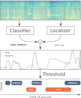
Many recent works on semi-supervised polyphonic SED rely on the workflow shown in Figure 1. A time/frequency representation ex-tracted from each audio file is used as input of two neural networks, a classifier, and a localizer. The classifier outputs binary vectors rep-resenting the classes of the sound events detected in a file, namely audio tags. The localizer outputs a matrix containing the probabil-ity values for each class and each temporal frame. A segmentation algorithm is used on these probabilities to output the sound event temporal markers.
2.2. Related work
In different works [2, 11], the authors do not mention what post-processing methods are used. In [1], the authors report tests of eight thresholds varying from 0.1 to 0.9. Lately, a mean-teacher model based on Recurrent Neural Networks (RNN) [12] won the DCASE 2018 challenge on large-scale weakly-labeled SED [13]. Nevertheless, very few details are given on the post-processing pro-cess. In [14], Convolutional RNNs were used to make predictions
.
DOG
t ime(10 secondes)
classes
SPEECH SPEECH SPEECH
DOG DOG, SPEECH (431, 10) Threshold Dog Speech Classi✁er Localizer
Figure 1: Semi-supervised polyphonic sound event detection work-flow illustrated for dog and speech event types as examples.
of pseudo-strong labels using median/Gaussian filters. These fil-ters are mentioned but not fully described. In [15], more details are given regarding which parameters must be tuned and how. The authors tested only absolute thresholding and median filtering. In other cases, simple threshold values are tuned on a development subset of the training data, such as in [16, 17].
In [3], Xia et al. addressed the issue of threshold selection in the context of polyphonic SED. The benchmark system is a Deep Neural Network (DNN) based on [4] and trained with bi-nary cross-entropy as loss function. To estimate thresholds for the post-processing step, the authors proposed two approaches, named contour-based and regressor-based methods, that estimate a thresh-old value for each frame. In the first one, the threshthresh-old is computed as the product between a coefficient α, which is set globally and expresses the ratio of non-empty frames, and the maximum values of the probabilities for each class. The second one uses a regres-sion to estimate the thresholds, based on an RNN, given as input the acoustic features and as a target, the probabilities output by the DNN. Both approaches rely on a precisely labeled training set that contains the time boundaries of each sound event.
Finally, aside from this last work, post-processing methods are often overlooked and not carefully evaluated. To our knowledge, there is no systematic analysis of the impact of post-processing within the sound event detection task. We suppose that many re-search works could benefit from a clear presentation of the ap-proaches as well as a detailed evaluation.
3. POST-PROCESSING METHODS
This section presents the proposed post-processing approaches, namely smoothing, segmenting and optimizing. They are described in-depth in the toolbox documentation online.
Smoothing removes noise in the probabilities, limiting the num-ber of small segments and small gaps created during the seg-mentation process. We use a smoothed moving average to do
so, with class-independent or class-dependent smoothing window sizes. These can be optimized with our toolbox.
3.1. Segmentation
3.1.1. statistics-based methods
The statistics-based methods are directly based on the statistics ex-tracted from the temporal predictions of each sample. The main ad-vantage of these methods is that they are fast and often efficient. i) class-independent data-wise average (CIDWA); ii) class-dependent data-wise average (CDDWA). We also tested class-(in)dependent file-wise average and median. However, those methods will not be mentioned as they yield either poor results (file-wise aver-age/median) or slightly worse results (data-wise median).
(i) CIDWA: we use the localizer outputs to compute the average probability of each class over time. We aggregate the averages to create a single threshold for all the classes.
(ii) CDDWA: class-dependent averages are used as thresholds.
3.1.2. Parametric methods
The parametric methods require optimization. We optimized the parameters on the test set and used them on the evaluation set. They can be either class-independent or class-dependent. We tested three methods: i) (in)dependent absolute (CIA-CDA), ii) class-(in)dependent hysteresis (CIH - CDH), iii) class-class-(in)dependent slope (CIS - CDS).
(i) Absolute thresholding refers to directly applying a unique and arbitrary threshold to the temporal predictions without using their statistics. This na¨ıve approach still yields exploitable results that can get close to the best ones in some cases. It is also the approach with the shortest optimization time due to the unique parameter to optimize.
(ii) Hysteresis thresholding consists of two thresholds. One of them will be used to determine the onset of an event, and the second one its offset. This algorithm is used when probabili-ties are unstable and changing at a high pace. It should, there-fore, decrease the number of events detected by the algorithm and reduce the insertion and deletion rates, giving a better er-ror rate than the Absolute threshold approach.
(iii) The Slope-based method determines the start and end of a seg-ment by detecting fast changes in the probabilities over time. Fast-rising probabilities imply the start of a segment, and fast decreasing probabilities, its end. It is capable of detecting the end of segments even if the probabilities are high.
3.2. Optimization
The parametric methods regroup together the different algorithms that exploit arbitrary parameters to locate with precision sound events. The search for the best parameter combination is a meticu-lous work that is often not possible to automatize. Indeed, depend-ing on the number of parameters to tune, the search space growth is exponential and the execution time often exceeds reasonable times. Consequently, we implemented a dichotomic search algorithm.
For every parameter to tune, the user provides an initial search interval. The algorithm tries every combination with a coarse reso-lution and picks the one that yields the best score. From this com-bination, a new smaller interval is computed. The complete process
Block repeated 3
times
forw. GRU backw. GRU
*
**
Log Mel ✁lterbank coe✂cients: 64 bands - 431 frames
conv, 3.3, 4x1 Batch-normalization ReLU max-pooling, 1x4 (spatial) dropout, p=0.2 time-distrib, dense, 64 time-distrib, dense, 10 sigmoid SED, 1@431x10
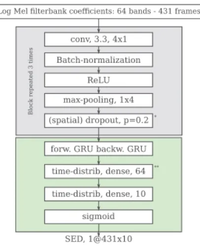
Figure 2: Architecture of MIL and Baseline. In Baseline, (∗) is a standard dropout layer (p = 0.3), and (∗∗) is removed.
is repeated with an increased precision and a reduced search space. It stops when the number of steps given by the user is reached.
The dichotomous search algorithm, when compared to an ex-haustive search of all the possible combinations, considerably re-duces the time needed to reach a near-optimal solution with excel-lent accuracy. However, the execution time is still dependent on the number of parameters to tune and the amount of iterations for every step. The total number of combinations increases exponentially.
4. EXPERIMENTS
4.1. Audio Material
The DCASE 2018 challenge task 4 [13] provided audio material directly extracted from Audioset. The training set is divided into three subsets. Only one of them is weakly annotated and we will refer to it as the ”weak” subset. The two others, being not annotated at all, are not of any use for the training of our models. The weak training subset is comprised of 1578 clips (2244 class occurrences) for which weak annotations have been verified and cross-checked.
The challenge also proposed a test and an evaluation subsets. Both of them have been strongly annotated, providing precise tem-poral segmentation (onset and offset boundaries) for each event oc-currence and are composed respectively of 279 and 880 files. Both of them present a similar distribution of the classes.
Each file can include one or several events from a set of sound classes occurring in domestic environments: Speech, Dog, Cat, Alarm/ Bell ringing, Dishes, Frying, Blender, Running water, Vac-uum cleaner, and Electric shaver/toothbrush. All the files are 10-second clips extracted from Audioset. These recordings contain generally several overlapping sound events from different classes.
The parametric methods will be optimized using the test dataset and validated on the evaluation dataset.
4.2. Models
To observe the impact of the segmentation algorithms, we used two approaches. The first one is similar to the DCASE 2018 base-line [18]. It uses a single RCNN to perform both audio tagging (AT) and segmenting. The second one is based on “Multiple Instance
Learning (MIL)” as proposed in [19, 20, 21]. It consists of two sep-arate networks: one for AT trained with standard cross-entropy and one for segmenting trained with a MIL objective.
The Baseline and MIL architecture is shown in Figure 2. It is composed of a convolutional part followed by a recurrent one, namely a bi-directional Gate Recurrent Unit layer and a time-distributed dense layer.
4.3. Experimental setup
Post-processing takes place after the model training phase, when thresholds are applied on smoothed time predictions to obtain the onset and offset of sound events. It is performed in the following or-der: 1) The curves representing the prediction of the model for each frame are smoothed using the smoothed moving average algorithm. This smoothing was applied only with the parametric methods since statistics-based methods are not meant to involve optimization. 2) the temporal predictions are segmented using one of the segmenta-tion algorithms described above. 3) Segments separated by a gap smaller than the challenge tolerance margin are merged together. In the same fashion, segments smaller than this margin are removed.
When a parametric method is used, the process is repeated to reach the best score by using the optimization algorithm. Sim-ilarly, the smoothing window size can be optimized either class-independently or class-dependently.
For both models, we tested the segmentation algorithms previ-ously described, as well as a coarse grid search that represents the combination of absolute thresholds from 0.1 to 0.9 and a 0.1 step, with smoothing window sizes from 5 to 21 and a step of 2, totaling 64 combinations. Two issues must be taken into consideration: i) the potential errors made by the audio tagging model, ii) the setting of parameter values when using a parametric method.
(i) To remove the bias induced by faulty audio tag classification, we used the classes of the strong annotations as if they were outputs from a perfect classifier. It allows us to pick only the relevant classes on which the events must be localized. We will refer to this mode as Audio Tagging oracle (AT oracle). We applied this procedure on both test and evaluation subsets. (ii) We used the event-based metrics defined in [22]. More pre-cisely the macro-F1 score, alias F1, with the challenge preci-sion parameters: a 200 ms collar on the onsets and an offset collar corresponding to 20% of the event’s length.
5. RESULTS
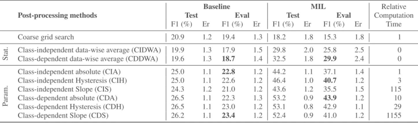
The results are presented in Table 1. Overall, they show a wide dis-parity in values. The F1 score varies from 17.9% to 23.4% with our baseline model, and from 25.8% to 43.9% with the MIL model. Therefore, we observe a significant impact of the post-processing algorithms on the final results. The best scores are obtained by us-ing the class-dependent parametric methods. On the evaluation set, CDS for our baseline gives a final F1 score of 23.4%, and CDA for the MIL model a final F1 score of 43.9%.
Regarding computation time, the best method is not necessarily the longest one and the gain, if there is any, is not linear. The base-line benefits only of 1.1 points for a computation time a thousand time longer, whereas MIL shows a decrease in performance. How-ever, the gain from class-independent to class-dependent is worth the extra time, which is in our case, approximately ten times more.
Post-processing methods
Baseline MIL Relative
Test Eval Test Eval Computation F1 (%) Er F1 (%) Er F1 (%) Er F1 (%) Er Time Coarse grid search 20.9 1.2 19.4 1.3 18.2 1.8 15.3 1.8 1
Stat.
Class-independent data-wise average (CIDWA) 19.9 1.3 17.9 1.5 29.8 2.0 25.8 2.5 0 Class-dependent data-wise average (CDDWA) 19.6 1.3 18.7 1.4 32.5 1.8 29.9 2.4 0 Class-independent absolute (CIA) 25.0 1.1 22.8 1.2 44.2 1.1 37.1 1.4 1 Class-independent Hysteresis (CIH) 25.0 1.1 22.6 1.2 46.4 1.0 40.7 1.2 3
P
aram.
Class-independent Slope (CIS) 24.3 1.2 21.0 1.2 43.6 1.2 35.5 1.5 115 Class-dependent absolute (CDA) 26.5 1.1 22.3 1.3 53.2 0.9 43.9 1.2 10 Class-dependent Hysteresis (CDH) 26.5 1.1 23.0 1.2 53.1 0.8 42.9 1.1 29 Class-dependent Slope (CDS) 26.2 1.1 23.4 1.2 52.4 0.9 41.0 1.2 1155
Table 1: F1-scores and Error Rates for both baseline and MIL on test and evaluation sets with the AT Oracle. The last column shows the relative computation time of each method compared to CIA.
With a closer look at statistics-based methods, CDDWA yields better performance with a final F1 score of 18.7% and 29.9% respectively on our baseline and MIL. In both cases, it gave better results on the evaluation subset than CIDWA. The Class-Dependent variant of the algorithm seems more suitable than the Class-Independent one even though it gave a slightly worse result on the test set (0.3 absolute difference). Indeed, If we look closely at the transition between test and evaluation sets, the difference is only of -4% for the dependent and -10% relative for the class-independent, making the first more robust.
Ultimately, the parametric methods present the best results. They perform better than the manually chosen threshold and the statistics-based ones. Furthermore, the best scores are obtained us-ing their class-dependent variant. The same observation can be done between the test and evaluation sets as the difference is only of -8% for class-dependent, and -18% for class-independent, making the class-dependent method not only perform better but also more ro-bust. Our baseline reaches on Eval a final F1 score of 23.4% with CDS. It represents an improvement of 4 points (20.6% relative). For MIL, the CDA method yields the best final F1 score with an improvement of 28.6 points (187.0% relative). The best Er value on Eval is 1.1% obtained with CDH.
If the statistics-based methods have already shown improve-ment of the final F1 score, the parametric ones push it even further, especially the class-dependent variants. The maximum F1 scores for the statistics-based methods are 18.7% and 29.9% for Baseline and MIL, respectively, to be compared with the parametric ones of 23.4% and 43.9%.
Regarding smoothing, in the class-dependent parametric meth-ods, the smoothing window size is a parameter that can be op-timized. A closer look at the parameter combination resulting from the optimization shows a wide variety of window size from 9 (Dishes) to 27 (Vacuum cleaner) frames. This highlights the im-portance of smoothing the predictions according to the classes.
When looking at the scoring of each class independently, the improvement is uniformly dispatched. When optimizing the algo-rithm parameters specifically for each class, (class-dependent para-metric methods), almost every class seems to benefit from the opti-mization, but few do not. It is the case with the class dishes.
Finally, we applied these methods on our model without us-ing the AT Oracle but the audio tags output by their classifier. We then compared it to the best models from the DCASE 2018 task 4
challenge. After optimization, the baseline F1 score increases from 12.6% to 14.1 (CDH) %, and for MIL, from 21.1% to 32.0% (CDH). The first [12] and the second [17] ranked participants obtained an F1 score of 32.4% and 29.9%, respectively.
6. CONCLUSION
In SED, prediction post-processing is often overlooked. There is no systematic analysis of its impact, and we compare several so-lutions to this problem. We explored several methods to segment the temporal prediction outputs from DNN-based models that can be divided into two categories: statistics-based and parametric ap-proaches, either class-independent or class-dependent.
The methods presented show the impact post-processing can have on the final performance. statistics-based methods do not re-quire optimization, making them suitable for a quick preview of the results that can be achieved. They are model-agnostic, easy to implement, fast to compute and can produce better results than a coarse grid search of the smoothing and thresholding parameters.
The parametric methods are nonetheless better. Our best model shows an improvement of 28.6 points (187.0% relative) by using the class-dependent absolute method. The class-dependent methods do not only yield better results but also greater robustness when switching from the test set to the evaluation set. For our submission to the DCASE 2019 Task 4 challenge, we obtain our best result with CDH. We reached rank four with a single small RCNN [23].
When it comes to the numerous datasets available nowadays, a larger one could be used to scale these methods and confirm their relevance. The same applies to the vast variety of models that have been implemented for SED tasks. Furthermore, other optimiza-tion techniques relying on genetic algorithms and probabilistic ap-proaches could be added to the ones tested in this work.
7. ACKNOWLEDGMENT
This work was partially supported by the Agence Nationale de la Recherche LUDAU (Lightly-supervised and Unsupervised Discov-ery of Audio Units using Deep Learning) project (ANR-18-CE23-0005-01). Experiments presented in this paper were carried out us-ing the OSIRIM platform that is administered by IRIT and sup-ported by CNRS, the Region Midi-Pyr´en´ees, the French Govern-ment, ERDF (see http://osirim.irit.fr/site/en).
8. REFERENCES
[1] E. Cakir, T. Heittola, H. Huttunen, and T. Virtanen, “Poly-phonic sound event detection using multi label deep neural networks,” in Proc. IJCNN. Killarney: IEEE, 2015, pp. 1–7. [2] G. Parascandolo, H. Huttunen, and T. Virtanen, “Recurrent neural networks for polyphonic sound event detection in real life recordings,” in Proc. ICASSP. Shanghai: IEEE, 2016, pp. 6440–6444.
[3] X. Xia, R. Togneri, F. Sohel, and D. Huang, “Frame-wise dynamic threshold based polyphonic acoustic event detection,” in Proc. Interspeech, Stockholm, 2017, pp. 474–478. [Online]. Available: http://dx.doi.org/10.21437/ Interspeech.2017-746
[4] Q. Kong, I. Sobieraj, W. Wang, and M. Plumbley, “Deep neu-ral network baseline for DCASE challenge 2016,” Budapest, 2016.
[5] L. Ballan, A. Bazzica, M. Bertini, A. Del Bimbo, and G. Serra, “Deep networks for audio event classification in soccer videos,” in Proc. ICME. Cancun: IEEE, 2009, pp. 474–477. [Online]. Available: http://dl.acm.org/citation.cfm? id=1698924.1699041
[6] D. Barchiesi, D. Giannoulis, D. Stowell, and M. D. Plumbley, “Acoustic scene classification: Classifying environments from the sounds they produce,” IEEE Signal Processing Magazine, vol. 32, no. 3, pp. 16–34, 2015.
[7] A. Harma, M. F. McKinney, and J. Skowronek, “Automatic surveillance of the acoustic activity in our living environ-ment,” in Proc. Multimedia and Expo. Amsterdam: IEEE, 2005.
[8] Y. LeCun, Y. Bengio, and G. Hinton, “Deep learning,” nature, vol. 521, no. 7553, pp. 436–444, 2015.
[9] T. Virtanen, M. D. Plumbley, and D. Ellis, Computational analysis of sound scenes and events. Springer, 2018. [10] J. F. Gemmeke, D. P. Ellis, D. Freedman, A. Jansen,
W. Lawrence, R. C. Moore, M. Plakal, and M. Ritter, “Audio set: An ontology and human-labeled dataset for audio events,” in Proc. ICASSP. New Orleans: IEEE, 2017, pp. 776–780. [11] Y. Guo, M. Xu, J. Wu, Y. Wang, and K. Hoashi,
“Multi-scale convolutional recurrent neural network with ensemble method for weakly labeled sound event detection,” DCASE Challenge, Woking, Tech. Rep., 2018.
[12] L. JiaKai, “Mean Teacher Convolution System for DCASE 2018 Task 4,” DCASE Challenge, Woking, Tech. Rep., 2018. [13] R. Serizel, N. Turpault, H. Eghbal-Zadeh, and A. P. Shah, “Large-scale weakly labeled semi-supervised sound event detection in domestic environments,” in Proc. DCASE, Woking, 2018, pp. 19–23. [Online]. Available: https: //hal.inria.fr/hal-01850270
[14] K. Koutini, H. Eghbal-zadeh, and G. Widmer, “Iterative knowledge distillation in r-cnns for weakly-labeled semi-supervised sound event detection,” DCASE Challenge, Wok-ing, Tech. Rep., 2018.
[15] R. Harb and F. Pernkopf, “Sound event detection using weakly labeled semi-supervised data with gcrnns, vat and self-adaptative label refinement,” DCASE Challenge, Woking, Tech. Rep., 2018.
[16] Y. Hou and S. Li, “Semi-supervised sound event detection with convolutional recurrent neural network using weakly la-belled data,” DCASE Challenge, Woking, Tech. Rep., 2018. [17] Y. L. Liu, J. Yan, Y. Song, and J. Du, “USTC-NELSLIP
Sys-tem For Dcase 2018 Challenge Task 4,” Challenge, Woking, Tech. Rep., 2018.
[18] R. Serizel, N. Turpault, H. Eghbal-Zadeh, and A. Parag Shah, “Large-scale weakly labeled semi-supervised sound event de-tection in domestic environments,” in Proc. DCASE, Woking, 2018.
[19] J. Salamon, B. McFee, P. Li, and J. P. Bello, “Multiple in-stance learning for sound event detection,” DCASE Chal-lenge, Munich, Tech. Rep., 2017.
[20] L. Cances, T. Pellegrini, and P. Guyot, “Sound event detection from weak annotations: weighted GRU versus multi-instance learning,” DCASE Challenge, Woking, Tech. Rep., 2018. [21] T. Pellegrini and L. Cances, “Cosine-similarity penalty to
dis-criminate sound classes in weakly-supervised sound event de-tection,” in Proc. IJCNN. Budapest: IEEE, 2019.
[22] A. Mesaros, T. Heittola, T. Virtanen, A. Mesaros, T. Heittola, and T. Virtanen, “Metrics for Polyphonic Sound Event Detection,” Applied Sciences, vol. 6, no. 6, p. 162, May 2016. [Online]. Available: http://www.mdpi.com/2076-3417/ 6/6/162
[23] L. Cances, T. Pellegrini, and P. Guyot, “Multi task learning and post processing optimization for sound event detection,” DCASE Challenge, New York, Tech. Rep., 2019.