Speaker Change Detection in Broadcast TV Using Bidirectional Long Short-Term Memory Networks

HAL Id: hal-01690244

https://hal.archives-ouvertes.fr/hal-01690244

Submitted on 23 Jan 2018

HAL is a multi-disciplinary open access

archive for the deposit and dissemination of

sci-entific research documents, whether they are

pub-lished or not. The documents may come from

teaching and research institutions in France or

abroad, or from public or private research centers.

L’archive ouverte pluridisciplinaire HAL, est

destinée au dépôt et à la diffusion de documents

scientifiques de niveau recherche, publiés ou non,

émanant des établissements d’enseignement et de

recherche français ou étrangers, des laboratoires

publics ou privés.

Speaker Change Detection in Broadcast TV Using

Bidirectional Long Short-Term Memory Networks

Ruiqing Yin, Hervé Bredin, Claude Barras

To cite this version:

Ruiqing Yin, Hervé Bredin, Claude Barras. Speaker Change Detection in Broadcast TV Using

Bidi-rectional Long Short-Term Memory Networks. Interspeech 2017, Aug 2017, Stockholm, Sweden.

�10.21437/Interspeech.2017-65�. �hal-01690244�

Speaker Change Detection in Broadcast TV

using Bidirectional Long Short-Term Memory Networks

Ruiqing Yin, Herv´e Bredin, Claude Barras

LIMSI, CNRS, Univ. Paris-Sud, Universit´e Paris-Saclay, F-91405 Orsay, France

firstname.lastname@limsi.fr

Abstract

Speaker change detection is an important step in a speaker di-arization system. It aims at finding speaker change points in the audio stream. In this paper, it is treated as a sequence label-ing task and addressed by Bidirectional long short term mem-ory networks (Bi-LSTM). The system is trained and evaluated on the Broadcast TV subset from ETAPE database. The result shows that the proposed model brings good improvement over conventional methods based on BIC and Gaussian Divergence. For instance, in comparison to Gaussian divergence, it produces speech turns that are 19.5% longer on average, with the same level of purity.

Index Terms: speaker diarization, speaker change detection, sequence labeling, recurrent neural network, LSTM

1. Introduction

Speaker diarization is the task of determining “who spoke when” in an audio stream that usually contains an unknown amount of speech from an unknown number of speakers [1, 2]. Speaker change detection is an important part of speaker di-arization systems. It aims at finding the boundaries between speech turns of two different speakers.

In recent years, the performance of state-of-the-art speech and speaker recognition systems has improved enormously thanks to the neural network (especially deep learning) ap-proaches. The proposed system in [3] has achieved human par-ity in conversational speech recognition. The key to this sys-tem’s performance is the systematic use of convolutional and Long Short-Term Memory (LSTM) neural networks. In speech recognition and natural language processing, LSTM has been used successfully for sequence labeling [4], language model-ing [5] and machine translation [6]. However, existmodel-ing speaker diarization systems do not take full advantages of these new techniques. [7] proposes an artificial neural network architec-ture to learn a feaarchitec-ture transformation from MFCCs that is op-timized for speaker diarization. However, the proposed system does not improve the initial change detection step, and rely on conventional methods presented in Section 2.

Our main contribution is introduced in Section 3 where we address speaker change detection as a binary sequence label-ing task uslabel-ing Bidirectional Long Short-Term Memory recur-rent neural networks (Bi-LSTM). Experiments on the ETAPE dataset are summarized in Section 4 and results are discussed in Section 5.

2. Related work

In conventional speaker change detection methods, one will use two adjacent sliding windows on the audio data, compute a dis-tance between them, then decide (usually by thresholding the distance) whether the two windows originate from the same

speaker. Gaussian divergence [8] and Bayesian Information Criterion (BIC) [9] have been used extensively in the literature to compute such a distance: they have both advantages of lead-ing to good segmentation results and not requirlead-ing any trainlead-ing step (other than for tuning the threshold).

There were some recent attempts at improving over these strong baselines with supervised approaches. Desplanques et al.[10] investigate factor analysis and i-vector for speaker seg-mentation. We recently proposed in [11] to train a recurrent neural network called TristouNet to project any speech seg-ment into a large-dimensional space where speech turns from the same (resp. different) speaker are close to (resp. far from) each other according to the euclidean distance. Replacing BIC or Gaussian divergence by the euclidean distance between Tris-touNetembeddings brings significant speaker change detection improvement. However, because they rely on relatively long ad-jacent sliding windows (2 seconds or more), all these methods tend to miss boundaries in fast speaker interactions.

Instead, we propose to address speaker change detection as a sequence labeling task, using LSTMs in the same way they have been successfully used for speech activity detection. In particular, our proposed approach is the direct translation of the work by Gelly et al. where they applied Bi-LSTMs on over-lapping audio sequences to predict whether each frame corre-sponds to a speech region or a non-speech one [12].

3. Speaker change detection as

a sequence labeling problem

Given an audio recording, speaker change detection aims at finding the boundaries between speech turns of different speak-ers. In Figure 1, the expected output of such a system would be the list of timestamps between spk1 & spk2, spk2 & spk1, and spk1 & spk4.

3.1. Sequence labeling

Let x ∈ X be the sequence of features extracted from the audio recording: x = (x1, x2...xT) where T is the total number of

features extracted from the sequence. Typically, x would be a sequence of MFCC features extracted on a short (a few millisec-onds) overlapping sliding window (aka. frame). The speaker change detection task is then turned into a binary sequence la-beling task by defining y = (y1, y2...yT) ∈ {0, 1}Tsuch that

yi = 1 if there is a speaker change during the ith frame, and

yi= 0 otherwise (see part B of Figure 1). The objective is then

to find a function f : X → Y that matches a feature sequence to a label sequence. We propose to model this function f as a recurrent neural network trained using the binary cross-entropy loss function: L = −1 T T X i=1 yilog(f (x)i) + (1 − yi) log(1 − f (x)i)

INTERSPEECH 2017

0 1 spk1 spk2 spk1 spk4 spk1 spk2 spk1 spk4 1 1 0 0 ... ... ... θ (A) (B) (C) (D) (E) (H) (G) (F) (I)

seg1 seg2 seg3 seg4

Figure 1: Training process (left) and prediction process (right) for speaker change detection. Details can be found in Section 3.

3.2. Network architecture

MLP

MLP

MLP

...

...

...

...

Figure 2: Model architecture

The actual architecture of the network f is depicted in Fig-ure 2. It is composed of two Bi-LSTM (Bi-LSTM 1 and 2) and a multi-layer perceptron (MLP) whose weights are shared across the sequence. Bi-LSTMs [13] allow to process sequences in for-ward and backfor-ward directions, making use of both past and fu-ture contexts. The output of both forward and backward LSTMs are concatenated and fed forward to the next layer. The shared MLP is made of three fully connected feedforward layers, using tanh activation function for the first two layers, and a sigmoid activation function for the last layer, in order to output a score between 0 and 1.

3.3. Class imbalance

Since there are relatively few change points in the audio files, very little frames are in fact labeled as positive (1). For in-stance, in the training of the ETAPE dataset used in the exper-imental section, this represents only 0.4% of all frames. This class imbalance issue could be problematic when training the neural network. Moreover, one cannot assume that human an-notation are precise at the frame level. It is likely that the actual location of speech turn boundaries is a few frames away from the one selected by the human annotators. This observation led most speaker diarization evaluation benchmarks [14, 15, 16] to remove from evaluation a short collar (up to half a second) around each manually annotated boundary. Therefore, as

de-picted in part C of Figure 1, the number of positive labels is increased artificially by labeling as positive every frame in the direct neighborhood of the manually annotated change point. We will further evaluate the impact of the size of this neighbor-hood in Section 5.

3.4. Subsequences

One well-publicized property of LSTMs is that they are able to avoid the vanishing gradients problem encountered by tradi-tional recurrent neural networks [17, 4]. Therefore, the initial idea was to train them on whole audio sequences at once but we found out that this has several limitations, including the lim-ited number of training sequences, and the computational cost and complexity of processing such long sequences with vari-able lengths. Consequently, as depicted in part D of Figure 1, the long audio sequences are split into short fixed-length over-lapping sequences. This has the additional benefit of increasing the variability and number of sequences seen during training, as is usually done with data augmentation for computer vision tasks. We will further discuss the advantages of this approach in Section 5.

3.5. Prediction

Once the network is trained, it can be used to perform speaker change detection as depicted in the right part of Figure 1. First, similarly to what is done during training, test files are split into overlapping feature sequences (part E of Figure 1). The net-work processes each subsequence to give a sequence of scores between 0 and 1 (part F of Figure 1). Because input sequences are overlapping, each frame can have multiple candidate scores; they are averaged to obtain the final frame-level score. Finally, local score maxima exceeding a pre-determined threshold θ are marked as speaker change points, as shown in part G of Fig-ure 1. Parts H and I respectively represent the hypothesized and groundtruth speaker change points.

4. Experiments

4.1. Dataset

The ETAPE TV subset [18] contains 29 hours of TV broadcast (18h for training, 5.5h for development and 5.5h for test) from three French TV channels with news, debates, and entertain-ment. Fine “who speaks when” annotations were provided on a

subset of the training and development set using the following two-steps process: automatic forced alignment of the manual speech transcription followed by manual boundaries adjustment by trained phoneticians. Overall, this leads to a training set of 13h50 containing N = 184 different speakers, and a develop-ment set of 4h10 containing 61 speakers (out of which 18 are also in the training set). Due to a coarser segmentation, the offi-cial test set is not used in this paper and the reported results are computed on the development set.

4.2. Implementation details

Feature extraction. 35-dimensional acoustic features are ex-tracted every 16ms on a 32ms window using Yaafe toolkit [19]: 11 Mel-Frequency Cepstral Coefficients (MFCC), their first and second derivatives, and the first and second derivatives of the energy.

Network architecture. The model stacks two Bi-LSTMs and a multi-layer perceptron. Bi-LSTM1 has 64 outputs (32 forward and 32 backward). Bi-LSTM2 has 40 (20 each). The fully connected layers are 40-, 10- and 1-dimensional respectively. Training. As introduced in Section 3, and unless otherwise stated, a positive neighborhood of 100ms (50ms on both sides) is used around each change point, to partially solve the class imbalance problem. Subsequences for training are 3.2s long with a step of 800ms (i.e. two adjacent sequences overlap by 75%). The actual training is implemented in Python using the Keras toolkit [20], and we use the SMORMS3 [21] optimizer. Baseline. Both BIC [9] and Gaussian divergence [8] baselines rely on the same set of features (without derivatives, because it leads to better performance), using two 2s adjacent windows. We also report the result obtained by the TristouNet approach, that used the very same experimental protocol [11].

4.3. Evaluation metrics

Conventional evaluation metrics for the speaker change detec-tion task are recall and precision. A hypothesized change point is counted as correct if it is within the temporal neighborhood of a reference change point. Both values are very sensitive to the actual size of this temporal neighborhood (aka. tolerance) – quickly reaching zero as the tolerance decreases. It also means that it is very sensitive to the actual temporal precision of human annotators.

Following what was done in [11], we propose to use purity and coverage evaluation metrics (as defined in pyan-note.metrics[22]) because they do not depend on a tolerance parameter and are more relevant in the perspective of a speaker diarization application. Purity [23] and coverage [24] were in-troduced to measure cluster quality but can also be adapted to the speaker change points detection task. Given R the set of reference speech turns, and H the set of hypothesized segments, coverage is defined as follows

coverage(R, H) = P r∈Rmaxh∈H|r ∩ h| P r∈R|r| (1) where |s| is the duration of segment s and r ∩ h is the intersec-tion of segments r and h. Purity is the dual metric where the role of R and H are interchanged. Over-segmentation (i.e. de-tecting too many speaker changes) would result in high purity but low coverage, while missing lots of speaker changes would

decrease purity – which is critical for subsequent speech turn agglomerative clustering.

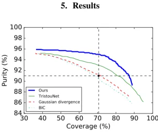
5. Results

30 40 50 60 70 80 90 100

Coverage (%)

84

86

88

90

92

94

96

98

100

Purity (%)

Figure 3: Speaker change detection on ETAPE development set All tested approaches (including the one we propose) rely on a peak detection step (keeping only those whose value is higher than a given threshold θ). Curves in Figure 3 were obtained by varying this very threshold θ. Our proposed so-lution clearly outperforms BIC-, divergence-, and TristouNet-based approaches, whatever the operating point. Notice how it reaches a maximum purity of 95.8%, while all others are stuck at 95.1%. This is explained by the structural limitations of ap-proaches based on the comparison of two adjacent windows: it is not possible for them to detect two changes if they belong to the same window. Our proposed approach is not affected by this issue.

BIC G.Div. TristouNet Ours 60.0 65.0 70.0 75.0 80.0 85.0 90.0 68.5 70.6 80.9 84.4 Coverage (%)

BIC G.Div. TristouNet Ours 90.0 91.0 92.0 93.0 94.0 95.0 96.0 90.5 91.0 93.0 94.7 Purity (%)

Figure 4: Left: coverage at 91.0% purity. Right: purity at 70.6% coverage.

Figure 4 summarizes the same set of experiments in a dif-ferent way, showing purity at 70.6% coverage, and coverage at 91.0% purity. Those two values are marked by the horizontal and vertical lines in Figure 3 and were selected because they correspond to the operating point of the divergence-based seg-mentation module of our in-house multi-stage speaker diariza-tion system [25]. Our approach improves both purity and cov-erage. For instance, in comparison to Gaussian divergence, it produces speech turns that are 19.5% longer on average, with the same level of purity.

We did try to integrate our contribution into our in-house speaker diarization system. Unfortunately, the overall impact on the complete system in terms of diarization error rate is very limited. This may be because the subsequent clustering module was optimized jointly with the divergence-based segmentation step, expecting a normal distribution of features in each segment

– which has no reason to be true for the ones obtained through the use of LSTMs.

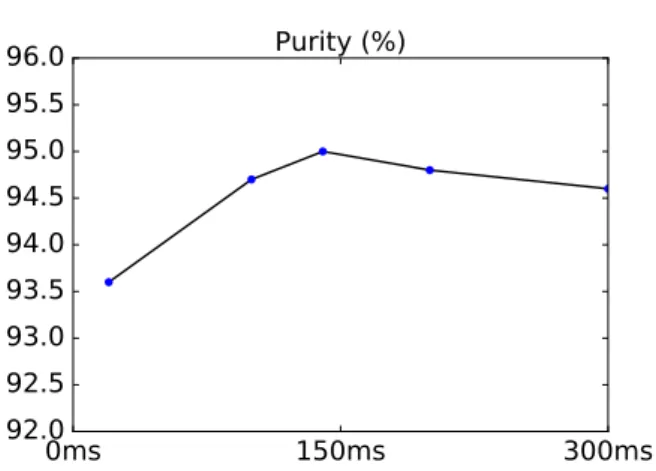
5.1. Fixing class imbalance

0ms

150ms

300ms

92.0

92.5

93.0

93.5

94.0

94.5

95.0

95.5

96.0

Purity (%)

Figure 5: Purity at 70.6% coverage for different balancing neighborhood size

As discussed in Section 3, to deal with the class imbalance problem, we artificially increased the number of positive labels during training by labeling as positive every frame in the di-rect neighborhood of each change point. Figure 5 illustrates the influence of the duration of this neighborhood on the segmen-tation purity, given that coverage is fixed at 70.6%. It shows a maximum value for a neighborhood of around 140ms. One should also notice that, even without any class balancing ef-fort, the proposed approach is still able to reach 93.6% purity, outperforming the other three tested approaches: the class im-balance issue is not as problematic as we initially expected. 5.2. “The Unreasonable Effectiveness of LSTMs”

As Karpathy would put it1, the proposed approach seems un-reasonably effective. Even though LSTMs do rely on an inter-nal memory, it is still surprising that they perform that well for speaker change detection, given that, at a particular time step i, all they see is the current feature vector xi. We first thought

that concatenating features from adjacent frames would be ben-eficial, but this did not bring any significant improvement. The internal memory mechanism is powerful enough to collect and keep track of contextual information.

This is further highlighted in Figure 6 that plots the ex-pected absolute difference between predicted scores f (x)i ∈

[0, 1] and reference labels yi ∈ {0, 1}, as a function of the

po-sition i in the sequence: δ(i) = Ex,y(|f (x)i− yi|). It clearly

shows that the proposed approach performs better in the mid-dle than at the beginning or the end of the sequence, quickly reaching a plateau as enough contextual information has been collected. This anticipated behavior justifies after the fact the use of strongly overlapping subsequences – making sure that each time step falls within the best performing region at least once. 1_{karpathy.github.io/2015/05/21/rnn-effectiveness}

0s

1.6s

3.2s

5.0

5.5

6.0

6.5

7.0

100

δ

(

i

)

Figure 6: Expected absolute difference between prediction score and reference label, as a function of the position in the 3.2s subsequence.

6. Conclusion and future work

We have developed a speaker change detection approach using bidirectional long short-term memory networks. Experimental results on the ETAPE dataset led to significant improvements over conventional methods (e.g., based on Gaussian divergence) and recent state-of-the-art results based on TristouNet embed-dings ( [11] also using LSTMs).

While neural networks are often considered as “magic” black boxes, we tried in Section 5.2 to better understand why these approaches are so powerful, despite their apparent sim-plicity. Yet, a lot remains to be done to really fully under-stand how the internal memory cells are actually used to gather and use the contextual information needed for detecting speaker changes.

Finally, despite major improvements of the speaker change detection module, its impact on the overall speaker diarization system is minor, possibly because segments obtained by LSTMs are not adapted to standard BIC- or CLR-based speaker diariza-tion approach. We plan to investigate LSTM-based speech turn embeddings like TristouNet to fully benefit from this improved segmentation.

7. Reproducible research

Code to reproduce the results of this paper is available here: github.com/yinruiqing/change_detection

8. Acknowledgements

This work was partly supported by ANR through the ODESSA (ANR-15-CE39-0010) and MetaDaTV (ANR-14-CE24-0024) projects. We thank M. Gregory Gelly for sharing useful ideas and experience on Bi-LSTM networks applied to speech pro-cessing.

9. References

[1] S. E. Tranter and D. A. Reynolds, “An overview of auto-matic speaker diarization systems,” IEEE Transactions on audio, speech, and language processing, vol. 14, no. 5, pp. 1557–1565, 2006.

[2] X. Anguera, S. Bozonnet, N. Evans, C. Fredouille, G. Fried-land, and O. Vinyals, “Speaker diarization: A review of recent research,” IEEE Transactions on Audio, Speech, and Language Processing, vol. 20, no. 2, pp. 356–370, 2012.

[3] W. Xiong, J. Droppo, X. Huang, F. Seide, M. Seltzer, A. Stolcke, D. Yu, and G. Zweig, “Achieving Human Parity in Conversational Speech Recognition,” Tech. Rep., February 2017. [Online]. Avail-able: https://www.microsoft.com/en-us/research/publication/ achieving-human-parity-conversational-speech-recognition-2/ [4] A. Graves, “Neural Networks,” in Supervised Sequence Labelling

with Recurrent Neural Networks. Springer, 2012, pp. 15–35. [5] M. Sundermeyer, R. Schl¨uter, and H. Ney, “LSTM Neural

Net-works for Language Modeling.” in Interspeech 2012, 13th Annual Conference of the International Speech Communication Associa-tion, 2012, pp. 194–197.

[6] I. Sutskever, O. Vinyals, and Q. V. Le, “Sequence to sequence learning with neural networks,” in Advances in neural information processing systems, 2014, pp. 3104–3112.

[7] S. H. Yella, A. Stolcke, and M. Slaney, “Artificial neural network features for speaker diarization,” in Spoken Language Technology Workshop (SLT), 2014 IEEE. IEEE, 2014, pp. 402–406. [8] M. A. Siegler, U. Jain, B. Raj, and R. M. Stern, “Automatic

seg-mentation, classification and clustering of broadcast news audio,” in Proc. DARPA speech recognition workshop, vol. 1997, 1997. [9] S. Chen and P. Gopalakrishnan, “Speaker, environment and

chan-nel change detection and clustering via the bayesian information criterion,” in Proc. DARPA Broadcast News Transcription and Understanding Workshop, vol. 8. Virginia, USA, 1998, pp. 127– 132.

[10] B. Desplanques, K. Demuynck, and J.-P. Martens, “Factor anal-ysis for speaker segmentation and improved speaker diarization,” in Interspeech 2015, 16th Annual Conference of the International Speech Communication Association, 2015, pp. 3081–3085. [11] H. Bredin, “TristouNet: Triplet Loss for Speaker Turn

Embed-ding,” in ICASSP 2017, IEEE International Conference on Acous-tics, Speech, and Signal Processing, New Orleans, USA, March 2017.

[12] G. Gelly and J.-L. Gauvain, “Minimum word error training of RNN-based voice activity detection.” in Interspeech 2015, 16th Annual Conference of the International Speech Communication Association, 2015, pp. 2650–2654.

[13] A. Graves, N. Jaitly, and A.-r. Mohamed, “Hybrid speech recogni-tion with deep bidirecrecogni-tional LSTM,” in Automatic Speech Recog-nition and Understanding (ASRU), 2013 IEEE Workshop on. IEEE, 2013, pp. 273–278.

[14] J. G. Fiscus, N. Radde, J. S. Garofolo, A. Le, J. Ajot, and C. Laprun, “The Rich Transcription 2005 spring meeting recogni-tion evaluarecogni-tion,” in Internarecogni-tional Workshop on Machine Learning for Multimodal Interaction (MLMI). Springer, 2005, pp. 369– 389.

[15] O. Galibert, J. Leixa, G. Adda, K. Choukri, and G. Gravier, “The ETAPE speech processing evaluation.” in LREC, 2014, pp. 3995– 3999.

[16] O. Galibert, “Methodologies for the evaluation of speaker diariza-tion and automatic speech recognidiariza-tion in the presence of over-lapping speech.” in Interspeech 2013, 14th Annual Conference of the International Speech Communication Association, 2013, pp. 1131–1134.

[17] S. Hochreiter and J. Schmidhuber, “Long short-term memory,” Neural computation, vol. 9, no. 8, pp. 1735–1780, 1997. [18] G. Gravier, G. Adda, N. Paulson, M. Carr´e, A. Giraudel,

and O. Galibert, “The ETAPE corpus for the evaluation of speech-based TV content processing in the French language,” in LREC - Eighth international conference on Language Resources and Evaluation, Turkey, 2012, p. na. [Online]. Available: https://hal.archives-ouvertes.fr/hal-00712591

[19] B. Mathieu, S. Essid, T. Fillon, J. Prado, and G. Richard, “YAAFE, an Easy to Use and Efficient Audio Feature Extraction Software.” in ISMIR 2010, 11th International Society for Music Information Retrieval Conference, 2010, pp. 441–446.

[20] F. Chollet, “Keras,” 2015. [Online]. Available: https://github. com/fchollet/keras

[21] S. Funk, “Rmsprop loses to SMORMS3,” 2015. [Online]. Available: http://sifter.org/∼_{simon/journal/20150420.html}

[22] H. Bredin, “pyannote.metrics: a toolkit for reproducible evaluation, diagnostic, and error analysis of speaker diarization systems,” in Interspeech 2017, 18th Annual Conference of the International Speech Communication Association, Stockholm, Sweden, August 2017. [Online]. Available: http://pyannote. github.io/pyannote-metrics

[23] M. Cettolo, “Segmentation, classification and clustering of an Ital-ian broadcast news corpus,” in Content-Based Multimedia Infor-mation Access-Volume 1, 2000, pp. 372–381.

[24] J.-L. Gauvain, L. Lamel, and G. Adda, “Partitioning and transcrip-tion of broadcast news data.” in ICSLP 1998, 5th Internatranscrip-tional Conference on Spoken Language Processing, vol. 98, no. 5, 1998, pp. 1335–1338.

[25] C. Barras, X. Zhu, S. Meignier, and J. L. Gauvain, “Multi-Stage Speaker Diarization of Broadcast New,” IEEE Transactions on Audio, Speech and Language Processing, vol. 14, no. 5, pp. 1505– 1512, Sep. 2006.