HAL Id: hal-03034529
https://hal.archives-ouvertes.fr/hal-03034529
Submitted on 1 Dec 2020
HAL is a multi-disciplinary open access
archive for the deposit and dissemination of
sci-entific research documents, whether they are
pub-lished or not. The documents may come from
teaching and research institutions in France or
abroad, or from public or private research centers.
L’archive ouverte pluridisciplinaire HAL, est
destinée au dépôt et à la diffusion de documents
scientifiques de niveau recherche, publiés ou non,
émanant des établissements d’enseignement et de
recherche français ou étrangers, des laboratoires
publics ou privés.
Implementation of polarization processes in a charge
transport model using time and frequency domain
measurements on PEN films
M-Q Hoang, Séverine Le Roy, Laurent Boudou, G. Teyssedre
To cite this version:
M-Q Hoang, Séverine Le Roy, Laurent Boudou, G. Teyssedre. Implementation of polarization
pro-cesses in a charge transport model using time and frequency domain measurements on PEN films. 9e
Conférence Société Française d’Electrostatique (SFE), Toulouse, France, 27-29 Aout 2014, Aug 2014,
Toulouse, France. pp. 384-389. �hal-03034529�
Implementation of polarization processes in a charge transport model
using time and frequency domain measurements on PEN films
M-Q. Hoang1*, S. Le Roy1,2, L. Boudou1 and G. Teyssèdre1,2
1 Université de Toulouse ; UPS, INPT ; LAPLACE (Laboratoire Plasma et Conversion d’Energie)
118 route de Narbonne, F-31062 Toulouse cedex 9, France
2 CNRS; LAPLACE; F-31062 Toulouse, France
* E-mail: maiquyen.hoang@laplace.univ-tlse.fr
Abstract: The aim of this work is to highlight the
polarization mechanisms in the time- and frequency-domains, and to implement the contribution of the polarization to the dielectric response into a charge transport model. To do so, Alternate Polarization Current (APC) and Dielectric Spectroscopy (DS) measurements have been performed on poly(ethylene naphthalene 2,6-dicarboxylate) (PEN), an aromatic polar material, providing information on polarization mechanisms in the time-domain and frequency-domain respectively. In the frequency-domain PEN exhibits 3 relaxation processes termed β, β* (sub-glass transitions) and α relaxations (glass transition) in increasing order of temperature. Conduction was also detected at high temperatures. Dielectric responses were treated using a simplified version of the Havriliak-Negami (HN) model (Cole-Cole (CC) model), using 3 parameters per relaxation process, function of the temperature. The time dependent permittivity obtained from the CC model is then added to a charge transport model. Simulated currents issued from the transport model implemented with the polarization are compared to the measured APC currents, showing a good consistency between experiments and simulations in a situation where the response is essentially from dipolar processes.
INTRODUCTION
An activity of modeling charge transport in insulators under electrical stress [1] was initiated by Le Roy et al ten years ago. A one-dimensional and bipolar model, able to describe transport, trapping and recombination of electronic carriers (electrons and holes) on the basis of experimental results has been developed. This model already gives good results on low density polyethylene (LDPE). However improvements are still possible, especially in order to predict the behavior of the space charge for different dielectric materials, particularly polar ones, under any electrical stress. The study of the variation of the material permittivity (ε) is necessary to take into account the polarization phenomena in the modeling. The permittivity depends on the experimental constraints (temperature, electrical field and polarization time) and its characterization can be done in the time-domain (Thermo-Stimulated Depolarization Current measurements –TSDC as an example) and in the frequency-domain (Impedance Spectroscopy
measurements). Whatever the characterization domain, time or frequency, the treatment of the experimental data to obtain the material relative permittivity remains difficult [2].
Poly(ethylene naphthalene 2,6-dicarboxylate) (PEN) has been chosen for this study as it is an aromatic polar polymer, and is known to give a significant response from dipolar mechanisms [3][4] for different measurements techniques. In our work, dielectric spectroscopy (DS) measurements, a well-known technique for performing a complete characterization of the dielectric relaxations, were carried out in order to characterize the polar response of the material in the frequency-domain. This response is then fitted with the help of Havriliak-Negami functions and introduced into a charge transport model. The model results are validated at different temperatures by current measurements under a low field (Alternate Polarization Current -APC- [5]).
DS MEASUREMENTS AND DATA PROCESSING Sample and measurement protocols
Semi-crystalline PEN films were commercial TEONEX® Q51 films provided by DuPont Teijin Films Co. The melting temperature is of 269°C and the glass transition temperature of 121°C [6]. Test films of 188 µm thickness were coated on each face with 16mm-diameter circular gold electrodes. DS measurements were carried out using a Novocontrol spectrometer over a frequency range going from 10-1 to 106 Hz, and for a
temperature range from -100 to 200°C by step of 5°C.
Experimental results
Dielectric results are shown in Fig. 1 as a function of frequency for different temperatures. The dielectric constant ε’ (Fig. 1a) weakly decreases over the frequency range, while it increases with the temperature. Fig. 1b shows the imaginary part of permittivity, dielectric loss, ε” vs. log(frequency) as a function of temperature. Three relaxation peaks are observed. The first one, called β, is assigned to local fluctuations of ester groups (O-C=O) similar to the β-process in Poly(ethylene terephthalate) (PET) [7]-[8]. The second peak, called β*, has been ascribed to the relative motion 9ème conférence de la Société Française d’Électrostatique, 27-29 août 2014, Toulouse, France.
of the two naphthalene rings present in the polymer chain [9]. The third peak, called α, has been related to the glass transition of PEN, involving long-range cooperative segments motion [10]. The α-relaxation is naturally originating from a conformational collective rearrangement of the chains in the amorphous regions of the material. The amplitude of the α-relaxation peak decreases as a result of crystallization [11]. Conduction was also detected after α-peak at 150°C in the low frequency range. β and β* peak maxima shift to higher frequencies when the temperature increases (Fig. 1). However, these three relaxations never appear simultaneously at a studied temperature. It is then necessary to model the global dielectric response of PEN, working on different temperature ranges for each relaxation.
Data processing by Cole-Cole functions
An empirical model of Havriliak and Negami [12] has been used to describe the dielectric relaxations. The variation of the complex permittivity ε*(ω)= ε’(ω)-j
ε”(ω) is given by:
*
1 2
( )
(1 ( ) )c c
j (1)
where ω=2πf is the electric field pulsation, Δε=εs-ε∞ is
the dielectric dispersion of the relaxation, εs and ε∞ are
the relaxed (ω=0) and unrelaxed (ω=∞) dielectric constant values, τ is the relaxation time associated with the relaxation, c1 and c2 (0≤c1, c2≤1) are shape parameters which describe the symmetric and the asymmetric broadening of the relaxation time distribution function, respectively. In the dielectric loss spectra of PEN, relaxation peaks are relatively symmetric. For this reason, we used the Cole-Cole function [13], a particular case of the Havriliak-Negami function with c2=1, to model the dielectric response. Taking into consideration the different relaxation modes and adding a conduction term to ε*, a complete function
is obtained: * 1 0 ( ) 1 ( )i ( ) n i c s i j i j (2) where c is similar to c1 in the Havriliak-Negami function, σ is ionic conduction term, ε0=8.85.10-12F.m-1
is the dielectric constant of vacuum, and s is a parameter related to the nature of the conduction mechanism (0≤s≤1). For PEN, 3 relaxations are observed (n=3), so there are 12 parameters that need to be fitted, and that are all temperature dependent.
In order to fit the global dielectric loss response of the semi-crystalline PEN, we used an extrapolation method, that was first proposed by Coburn et al. [8] for studying the relaxations of PET, and widely applied on PEN [2], [14]. The fit by a Cole-Cole function was done for all the temperatures where the maximum of dielectric loss was well defined in the experimental frequency window. The dielectric losses vs. frequency in the temperature region of the β-relaxation peak (from -80°C to -20°C) are presented in Fig. 2. It is to note that for this relaxation, the peak has been attributed in the literature as being the sum of two contributions, β1 and β2 [2],
[15]. However, for sake of simplification and as we already have a large number of parameters to extract, we fitted the β relaxation as a unique contribution.
-1 0 1 2 3 4 5 6 0.01 0.02 0.03 0.04 0.05 (b) (a)
"
log[f/Hz] 3.90 4.05 4.20 4.35 4.50'
-100°C -50°C 0 50°C 100°C 150°CFig. 1. Dielectric constant (a) and loss (b) vs. log(frequency) in PEN as a function of temperature
-1 0 1 2 3 4 5 6 0.01 0.02 0.03 0.04
"
log[f/Hz] -80°C -70°C -60°C -50°C -40°C -30°C -20°C regionFig. 2. Dielectric loss vs log(frequency) in region of β-relaxation for PEN.
For this β relaxation, a set of Cole-Cole parameters able to fit the dielectric loss and permittivity vs. frequency, was obtained. An example of comparison between the fit (line) and the experimental dielectric loss (symbols) vs. frequency at -50°C is given in Fig. 3a. The fit has been performed around the peak maximum (between the two vertical dashed lines on Fig. 3a) in order to avoid the possible contributions of other relaxations. These variations are described by equations (3)-(5):
-10 0.263 7.796.10 T (3) -3 0.065 1.452.10 - T c (4) 0.634 39.307 -ln B k T (5)
where T is the temperature, in K, kB=8.617.10-5eV.K-1 is
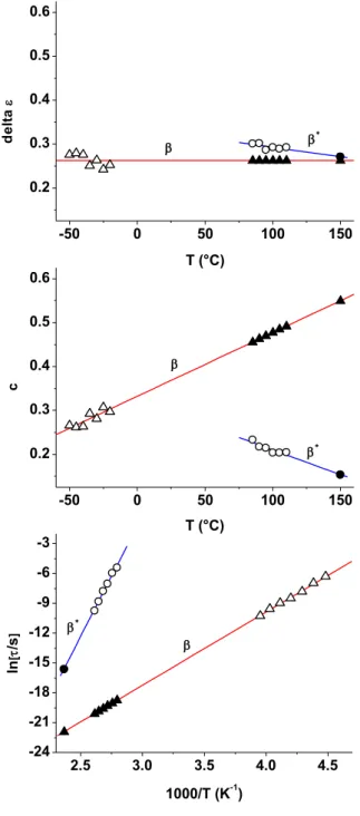
the Boltzmann constant. The set of parameters is presented in Fig. 4 (open triangles). ∆ε and c follow nearly a linear variation with temperature, while ln(τ) linearly increases with the reciprocal absolute temperature following the Arrhenius law.
For the β*-relaxation peak, the best approximations were
found for temperatures ranging from 85 to 110°C where the maximum of dielectric loss was well defined in the experimental frequency window. However, it is necessary to take into account the overlapping β-process for high frequencies. This was done by adding to the contribution of β*-peak the extrapolation of the
contribution of β-peak using equations (3)-(5) in the temperature region of β*-peak (filled triangles in Fig. 4).
The experimental values of ε” in this region were fitted using the equation:
" " " *
( ) ( ) ( ) (6)
Fig. 3b shows the fit result of β*-peak at 95°C
performed in the region of frequency from 1 to 106 Hz,
where the influence of α-process contribution can be neglected. By doing so for all the temperatures from 85 to 110°C, a set of Cole-Cole parameters for the β*-peak
was obtained. This set is presented in Fig. 4 (open circles), and fitted by equations (7)-(9).
4 * 0.456 4.352.10 T (7) 3 * 0.631 1.129.10 T c (8) 2.090 -72.958 ln B k T (9)
Finally, the similar procedure was used to obtain the parameters related to the α-relaxation and the conduction. In this case we used the equation:
" " " " " *
( ) ( ) ( ) ( ) ( ) (10)
The extrapolation of the contribution of β-peak and β* -peak was realized from equations (3)-(5) and (7)-(9) respectively in the temperature region of α-peak (filled triangles and filled circles in Fig. 4). Fig. 3c shows the fit result of dielectric loss at 150°C in full experimental frequency range with all contributions (β, β*, α and
conduction).
IMPLEMENTATION OF POLARIZATION IN THE CHARGE TRANSPORT MODEL
Charge transport model and equations
The charge transport model used to reproduce the behavior of space charge in PEN has already been presented in the literature [1] for polyethylene. It takes
0.00 0.02 0.04 0.06 0.08 0.10 150°C 95°C -50°C (b)
"
experimental data fit Cole-Cole(a) 0.00 0.02 0.04 0.06 0.08 0.10
"
-1 0 1 2 3 4 5 6 7 8 9 10 0.00 0.02 0.04 0.06 0.08 0.10 (c)"
log[f/Hz]Fig. 3. Dielectric loss for PEN as a function of temperature. Experimental data and fit results at: a. -50°C; b. 95°C; c. 150°C.
into account the injection of electronic charges (electrons and holes), their transport in the insulation volume, their trapping and recombination for each type of carrier. It allows having access to measurable macroscopic parameters that are net charge density, external current, surface potential, etc.
The model is based on Poisson, transport and continuity equations. Until now, the permittivity was considered in this model as a constant, regardless of the experimental conditions. In order to implement the variation of the permittivity in the charge transport model, Poisson
equation and the external current equation need to be rewritten as: ( , ) ( , ) D x t x t (11) ( , ) ( , ) ( , ) D x t J x t j x t x (12)
where ρ(x,t) is the net charge density, function of time and space, and jc(x,t) is the local conduction current.
D(x,t) is the electrical displacement, which includes the polarization and is given in the frequency domain by [16]:
* 0
( ) ( ) ( )
D E (13)
where E is the electric field, ε0 the vacuum permittivity
and ε*(ω) the material permittivity defined by Cole-Cole functions: * 1 1 ( ) ( ) 1 ( ) i n n i i i c i j i i (14) Including equation (14) into (13) gives:
0 0 1 ( ) ( ) ( ) ( ) n i i i D E E (15)
An inverse Fourier transform is then necessary to change the permittivity response from the frequency-domain to the time-frequency-domain. A particular attention should be paid during the data treatment on the sampling representativeness between frequency- and time-domain. Finally, applying the Laplace transform, taking into account E as a function of time and space, the electric displacement is obtained.
0 0 1 ( , ) ( , ) ( , ) * ( ) n i i i D x t E x t E x t t (16)
Current measurements at low fields (APC)
In order to validate the charge transport model, which now takes into account the time-dependent permittivity, alternate polarization current (APC) measurements [5] were carried out on PEN samples. The experimental protocol is presented in Fig. 5. Samples were polarized successively under electric fields E0 and -E0 during
several half-periods T/2. In order to avoid charge injection into the dielectric, very low electric field E was applied. The polarity change between each step decreases clearly the scattering of consecutive current [17]. In our study, test films of thickness 188 or 75 µm were coated on each face with a 60mm-diameter circular gold electrode. They were polarized under low electric fields, 0.05 kV/mm during 5 half-periods of
-50 0 50 100 150 0.2 0.3 0.4 0.5 0.6 c T (°C) -50 0 50 100 150 0.2 0.3 0.4 0.5 0.6 T (°C) de lt a 2.5 3.0 3.5 4.0 4.5 -24 -21 -18 -15 -12 -9 -6 -3 ln [ /s ] 1000/T (K-1)
Fig. 4. Cole-Cole parameters vs. temperature obtained from fit method and used as extrapolated data. Open symbols correspond to fitting parameters; filled symbols correspond to
extrapolated parameters. β-relaxation: triangles;; β*
1000s for a temperature range from ambient temperature to 90°C. At very low and high temperatures (-80, 130 and 150°C), a higher field was chosen (1.33 kV/mm during 2 half-periods of 1000s relative to 0.5 kV/mm) in order to decrease the noise of measured current.
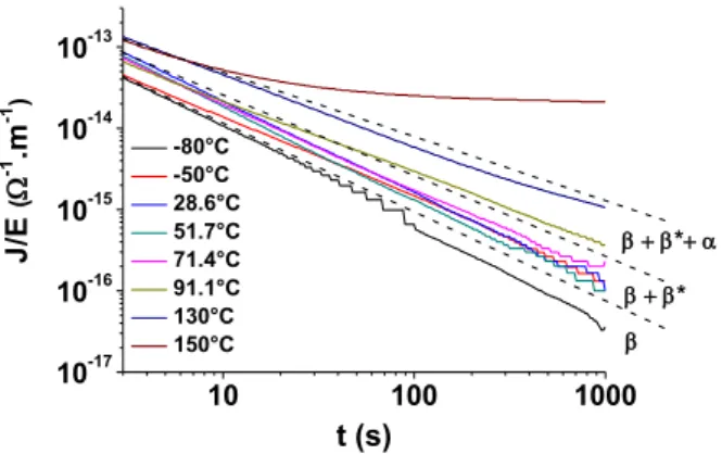
In a previous communication [3], we indicated that charges were not injected in PEN samples bulk under 10 kV/mm if the temperature did not exceed 130°C. Fig. 6 shows the normalized current densities obtained in PEN as a function of time for different temperatures. Depending on how many relaxation processes are at play, the polarization currents can be separated into 3 temperature regions: -80°C, from 28.6 to 71.4°C and from 91.1 to 130°C. The measured polarization currents correspond to the contributions of relaxations β, β* and
α that appear consecutively when the temperature is increased. The current curve at 150°C differs from that at other temperatures. Conduction becomes dominant at high temperatures and APC measurements no longer reflect polarization processes only.
Comparison of simulation and experimental results
Simulations were performed for electric fields following the protocol used for APC measurements and for temperatures ranging from -80 to 50°C. In a first attempt to validate our model, the injection and transport contributions were not taken into account. At
these low fields, and at relatively low temperatures, the conduction contribution should be low compared to polarization mechanisms and hence this hypothesis should hold. Hence, the external current in equation (12) is only due to the second part of the right hand side, i.e. to the variation of permittivity with time. Fig. 7 shows the comparison between simulated and experimental results (normalized currents) in the time-domain and for two temperatures: -80°C and 50°C. For both temperatures, at very low frequencies, the maximum of β- and β*-relaxation peaks were well defined in the
studied frequency-window. We can see that the simulations are in good agreement with the measurements in time-domain for two different temperatures, qualitatively and quantitatively.
CONCLUSION
Dielectric spectroscopy was used to characterize the polarization mechanisms in PEN. Three relaxation peaks were observed, β, β* and α, as polarization
contributions. The first two peaks are secondary relaxations, whereas the α-peak is related to the glass transition of the material. Polarization processes were implemented in a charge transport model on the basis of experimental results provided by dielectric spectroscopy in the frequency-domain. These experimental data were fitted using Cole-Cole functions prior to an inverse Fourier transform to get the permittivity variation in the time domain. Validation of the charge transport model including polarization mechanisms was performed by comparing simulated external current and low fields current obtained in time domain, where the response is essentially dipolar. This result allows validating the data processing from the frequency-domain to the time-domain. The implementation of the polarization in the charge transport model must now be used to account for the current values measured at short time and under high electric fields, or high temperatures, which are ascribed to polarization phenomena.
10 100 1000 10-17 10-16 10-15 10-14 10-13 * J/ E ( -1 .m -1 ) t (s) -80°C -50°C 28.6°C 51.7°C 71.4°C 91.1°C 130°C 150°C *
Fig. 6. APC profiles for PEN as a function of temperature.
Electric field (V/m) Time (s) 0 T 2 E0 -E0
Fig. 5. Electric field protocol of APC measurements.
10 100 1000 10-17 10-16 10-15 10-14 10-13 J/ E ( -1 .m -1 ) t (s) simulation at -80°C measurement at -80°C simulation at 50°C measurement at 51.7°C
Fig. 7. Comparison of normalized currents simulated by the charge transport model and APC normalized currents at -80 and 50°C.
REFERENCES
[1] S. Le Roy, G. Teyssedre, C. Laurent, G.C. Montanari, F. Palmieri, “Description of charge transport in polyethylene using a fluid model with a constant mobility: fitting model and experiments”, J. Phys. D.: Appl. Phys., Vol. 39, pp.1427-1436, 2006.
[2] S.P. Bravard and R.H. Boyd, “Dielectric Relaxation in Amorphous Poly(ethylene terephthalate) and Poly(ethylene 2,6-naphthalene dicarboxylate) and Their Copolymers”, Macromolecules, Vol. 36, pp. 741-748, 2003.
[3] M.Q. Hoang, L. Boudou, S. Le Roy, G. Teyssedre, “Electrical characterization of PEN films using TSDC and PEA measurements”, 2013 IEEE International Conference on Solid Dielectrics (Bologna, Italy), pp.488-491, 2013.
[4] J.C. Canãdas, J.A. Diego, M. Mudarra, J. Belana, R. Díaz-Calleja, M.J. Sanchis, C. Jaimés, “Relaxational study of poly(ethylene-2,6-naphthalene dicarboxylate) by t.s.d.c., d.e.a. and d.m.a.”, Polymer, Vol. 40, pp. 1181-1190, 1999.
[5] C. Escribe-Filippini, R. Tobazéon, J.C. Filippini, “Conduction characterization of polymer films using the alternate square wave method”, 7th IEEE International
Conference on Solid Dielectrics (Eindhoven,
Netherlands), pp. 315-318, 2001. [6] http://www.dupontteijinfilms.com
[7] B. Schartel and J.H. Wendorf, “Dielectric investigation on secondary relaxation of polyarylates: comparison of low molecular models and polymeric compounds”, Polymer, Vol. 36, pp. 899-904, 1995. [8] J.C. Coburn and R.H. Boyd, “Dielectric relaxation in poly(ethylene terephthalate)”, Macromolecules, Vol. 19, pp. 2238-2245,1986.
[9] H. Dortliz and H.G. Zachmann, “Molecular mobility in poly(ethylene-2,6-naphthalene dicarboxylate) as determined by means of deuteron NMR”, J. Macromol.. Sci. B: Phys., Vol. 36, pp. 205-219, 1997.
[10] J. Belana, M. Mudarra, J. Calaf, J.C. Canãdas, E. Menéndez, “Tsc study of the polar and free charge peaks of amorphous polymers”, IEEE Trans. Electr. Insul., Vol. 28, pp. 287-293, 1993.
[11] J.P. Bellomo and T. Lebey, “On some dielectric properties of PEN”, J. Phys. D.: Appl. Phys., Vol. 29, , pp. 2052, 1996.
[12] S. Havriliak and S. Negami, “A complex plane representation of dielectric and mechanical relaxation processes in some polymers”, Polymer, Vol. 8, pp. 161-210, 1967.
[13] K.S. Cole and R.H. Cole, “Dispersion and absorption in dielectrics: I. Alternating current characteristics”, J. Chem. Phys., Vol. 9, pp. 341-351, 1941.
[14] A. Nogales, Z. Denchev, I. Sics, T.A. Ezquerra, “Influence of Crystalline structure in the segmental mobility of semicrystalline polymers: poly(ethylene naphthalene-2,6-dicarboylate)”, Macromolecules, Vol. 33, pp. 9367-9375, 2000.
[15] C. Hakme, I. Stevenson, L. David, G. Boiteux, G. Seytre, A. Schönhals, “Uniaxially stretched poly(ethylene naphthalene 2,6-dicarboxylate) films studied by broadband dielectric spectroscopy”, J. Non-Cryst. Solids, Vol. 351, pp. 2742-2752, 2005.
[16] C.J.F. Böttcher and P. Bordewijk, “Theory of Electric Polarization, Vol. II: Dielectrics in time-dependent fields”, Verlag Elsevier, Amsterdam, 1978. [17] V. Adamec and J.H. Calderwood, “On the determination of electrical conductivity in polyethylene”, J. Phys. D: Appl. Phys., Vol. 14, pp. 1487-1494, 1981.