HAL Id: hal-00486839
https://hal.archives-ouvertes.fr/hal-00486839
Submitted on 26 May 2010
HAL is a multi-disciplinary open access
archive for the deposit and dissemination of
sci-entific research documents, whether they are
pub-lished or not. The documents may come from
teaching and research institutions in France or
abroad, or from public or private research centers.
L’archive ouverte pluridisciplinaire HAL, est
destinée au dépôt et à la diffusion de documents
scientifiques de niveau recherche, publiés ou non,
émanant des établissements d’enseignement et de
recherche français ou étrangers, des laboratoires
publics ou privés.
Simulator Generation Using an Automaton Based
Pipeline Model for Timing Analysis.
Rola Kassem, Mikaël Briday, Jean-Luc Béchennec, Yvon Trinquet, Guillaume
Savaton
To cite this version:
Rola Kassem, Mikaël Briday, Jean-Luc Béchennec, Yvon Trinquet, Guillaume Savaton. Simulator
Generation Using an Automaton Based Pipeline Model for Timing Analysis.. International
Multicon-ference on Computer Science and Information Technology (IMCSIT), International Workshop on Real
Time Software (RTS’08)., Oct 2008, Wisla, Poland. pp.657-664. �hal-00486839�
Simulator Generation Using an Automaton Based
Pipeline Model for Timing Analysis
Rola Kassem, Mika¨el Briday, Jean-Luc B´echennec, and Yvon Trinquet
IRCCyN, UMR CNRS 6597 1, rue de la No¨e - BP92101 44321 Nantes Cedex 3 - France [email protected]
Guillaume Savaton
ESEO
4, rue Merlet de la Boulaye - BP30926 49009 Angers Cedex 01 - France
Abstract—Hardware simulation is an important part of the design of embedded and/or real-time systems. It can be used to compute the Worst Case Execution Time (WCET) and to provide a mean to run software when final hardware is not yet available. Building a simulator is a long and difficult task, especially when the architecture of processor is complex. This task can be alleviated by using a Hardware Architecture Description Language and generating the simulator. In this article we focus on a technique to generate an automata based simulator from the description of the pipeline. The description is transformed into an automaton and a set of resources which, in turn, are transformed into a simulator. The goal is to obtain a cycle-accurate simulator to verify timing characteristics of embedded real-time systems. An experiment compares an Instruction Set Simulator with and without the automaton based cycle-accurate simulator.
I. INTRODUCTION
S
Imulation of the hardware platform takes place in the final stage of development. It can be used for 2 tasks. The first task is the evaluation of WCET to compute the schedulability of the application [9]. The second task is the test of the application using scenarios before final testing on the real hardware platform. This test is useful because simulation allows an easy analysis of the execution. In both cases, a cycle accurate model of the hardware platform must be used to insure that timings of the simulation are as close as possible to timings of the execution on the real platform.A common approach for the hardware modelling [5] is based on an hardware centric view; in this approach, the processor is usually modelled by a set of functional blocks. The blocks communicate and synchronise with each other in order to handle the pipeline hazards. A pipeline can be modelled with this approach by designing a functional block for each stage of the pipeline (a SystemC [8] module for instance). This approach is very useful in the design process as it allows synthesis generation. However, simulators that are generated from these kind of models are slow because of the block synchronisation cost. In our approach, we propose to use an Architecture Description Language (ADL) to describe the pipeline and the instruction set of the target architecture. The goal of the pipeline description is to focus on the effects of dependencies and device usage on the timing. This description
This work is supported by ANR (French National Research Agency) under Grant Number ADEME-05-03-C0121.
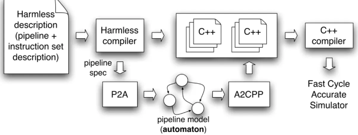
is transformed into a finite state automaton, which is then transformed into the simulator source code by adding the instruction behaviour (see figure 1). The aim of the automaton is to provide a faster - yet accurate - simulator because hazards of the pipeline are not computed at execution time but at generation time instead. This paper focuses on pipeline modelling and does present the pipeline description in our ADL: HARMLESS [7] (Hardware ARchitecture Modelling Language for Embedded Software Simulation) but the method presented may be extended to include the modelling of other parts of the architecture like branch prediction or cache memories.
II. RELATED WORK
Pipeline and resource scheduling have been studied widely in instruction schedulers, that are used by compilers to ex-ploit the instruction level parallelism and to minimise the program execution time. In [12], M¨uller proposes to use one or more finite state automata to model the pipeline and build a simulator. Then the simulator is used by the instruction scheduler to compute the execution time of instruction se-quences. The automata can be quite large and minimisation techniques may be used to alleviate them. In [13], Proebsting and Fraser use the same approach but a different algorithm which produces directly a minimal automaton. In [1], Bala and Rubin improve the algorithm on [12] and [13] by allowing to replace instructions in already scheduled sequences and present the BuildForwardFSA algorithm which is used to build the automaton. In these works, only structural hazards are taken into account. It makes sense for instruction schedulers. Other works have been done to build simulator for WCET analysis using an ADL. In [10], Li and al. use the EXPRES-SION ADL to build an executions graph and express pipeline hazards. The hazards are resolved at run-time. In [14], Tavares and al. use a minimal ADL to generate a model based on Proebsting and Fraser work.
In [2], another kind of pipeline modelling using coloured Petri Nets is presented, but functional behaviour is not taken into account. The simulator cannot execute a real binary code. In the work presented hereafter, we extend the BuildFor-wardFSA algorithm to take into account the data hazards (data dependency), the control hazards and the resources which can
pipeline model (automaton) A2CPP C++C++C++ C++ compiler Fast Cycle Accurate Simulator C++C++C++ Harmless compiler Harmless description (pipeline + instruction set description) pipeline spec P2A
Fig. 1. Development chain. Tools presented in this paper include p2a and a2cpp to transform a pipeline description into a fast simulator, using an automaton model.
be held by external hardware devices that are not modelled using one automaton.
The paper is organised as follow: Section III presents how the pipeline is modelled. The two kind of resources and their usage are described. Instruction classes are introduced. Section IV explains the automaton generation algorithm. In section V, a brief description of HARMLESS ADL with a focus on pipeline description, is given. Section VI presents examples. Section VII presents the simulation result provided by our approach. Section VIII explains the relation between simulation and WCET. At last, section IX concludes this paper.
III. PIPELINE MODELLING
Sequential pipelines are considered in this paper (i.e. there are no pipelines working in parallel nor forking pipelines). An automaton is used to model the pipeline behaviour where a state of the automaton represents the pipeline state at a particular time (see figure 2).
At each clock cycle, the pipeline goes from one state to another according to hazards. They are classified into three categories:
• Structural hazards are the result of a lack of hardware
resource;
• Data hazardsare the result of a data dependancy between
instructions;
• Control hazards that occurs when a branch is taken in
the program.
Control hazard are resolved in the simulator at runtime: instructions that are in the delay slot of a branch instruction are dynamically replaced by NOP instructions, if the branch is found to be taken. Constraints resulting from structural and data hazards are used to generate this automaton and modelled using resources.
A. Resources
Resourcesare defined as a mechanism to describe temporal constraints in the pipeline. They are used to take into account
structural hazardsand data hazards in the pipeline.
state 1 state 2 state 3 state 4 ... .. . D F E W E D W W D F E D F F ... ... D E W F D D E W F D E F D F D E W F D E W F ... i-1 i-2 t-4 t-5 s tat e 1 s tat e 2 s tat e 3 s tat e 4 s tat e 1 W E D F s tat e 1 ... i i+2 i+1 i+3 instructions time (cycles) t-3 t-2 t-1 t t+1 t+2
Fig. 2. A state of the automaton represents the state of the pipeline at a given time. In this example with a 4-stages pipeline, three instructions are in the pipeline at time t, and the ’D’ stage was stalled at time t-1. The automaton highlights the pipeline sequence, assuming that there is only one instruction type (this restriction is only made for clarity reason).
Two types of resources are defined, internal and external resources, that model constraints respectively statically and dynamically.
1) Internal resources: can be compared to “resources” in [12]. They model structural hazards.
As the pipeline state is known (i.e. the instructions are defined for each stage of the pipeline), then the state of each internal resource is fully defined (taken or available). In that case, when the automaton is built (and then the simulator), constraints described by internal resources are directly resolved when the set of next states is built.
Internal resources are designed to describe structural haz-ards inside a pipeline. As these resources are taken into ac-count at build time (static approach), no computation overhead is required to check for this type of constraint at runtime.
For example, each pipeline stage is modelled by an internal resource. Each instruction that enters in a stage takes the associated resource, and releases that resource when it leaves. The resulting constraint is that each pipeline stage gets at most one instruction. Another example of internal resource is presented in section VI.
2) External resources: represent resources that are shared with other hardware components such as timers or memory controllers. It is an extension of internal resources to take into account resources that must be managed dynamically (i.e. during the simulation). For instance, in the case of a memory controller, the pipeline is locked if it performs a request whereas the controller is busy. Otherwise, the pipeline stage that requests the memory access takes the resource.
If an external resource can be taken by instructions in more than one pipeline stage, a priority is set between stages. For example, at least two pipeline stages may compete for a memory access using a single pipelined micro-controller without instruction cache nor data cache.
One interesting property of the external resources is that it allows to check for data hazards. An external resource is used, associated to a data dependancy controller. In this section, we suppose that the first stages of the pipeline are a fetch stage, followed by a decode stage that reads operands.
The data dependancy controller works as presented in algorithm 1 when instructions in the pipeline are executed. An instruction that is in the Fetch stage sends a request to the controller to check if all of the operands, that will be taken in the next stage (Decode), are available. If at least one of the register is busy (because it is used by one or more instructions in the pipeline), the request fails and the associated external resource is set to busy.
When the transition’s condition is evaluated to get the next automaton state, the transition associated with this new condition (the transition’s condition depends of the state of external resources) will lead to a state that inserts a stall in the pipeline. It allows the instruction that is in the fetch stage to wait for its operands, and resolves the data dependancy.
Algorithm 1: Instructions and data dependancy controller interaction during simulation.
if there is an instruction in the fetch stage and the instruction
will need operands in the decode stage then
- The instruction sends a request to the controller; if at least one register is busy then
- the request fails: the external resource associated is set to busy;
else
- the request success: the external resource associated is set to available;
else
- the request success: the external resource associated is set to available;
B. Instruction class
To reduce the automaton state space, instructions that use the same resources (internal and external) are grouped to build instruction classes.
The number of instruction classes is limited to 2Rext+Rint (Rext and Rint are the number of respectively external and
internal resources in the system), but this maximum is not reached because some resources are shared by all instructions, like pipeline stages, which leads to get a lower number of instruction classes.
IV. GENERATING THE FINITE AUTOMATON
The automaton represents all the possible simulation sce-narios of the pipeline. A state of the automaton represents a state of the pipeline, which is defined as the list of all pair (instruction classes, pipeline stage) in the pipeline at a given time. For a system with c instruction classes, there are c+ 1 possible cases for each pipeline stage s of the pipeline (each instruction class or a stall). The automaton is finite because it has at most (c + 1)s
states. The initial state is the one that represents an empty pipeline. A transition is taken at each clock cycle and its condition depends only on:
• the state of the external resources (taken or available); • the instruction class of the next instruction that can be
fetched in the pipeline.
Internal resources are already resolved in the generated au-tomaton and does not appear in the transition’s condition. Other instructions in the pipeline are already known for a given automaton state, thus only the next instruction that will be fetched is necessary. This transition’s condition is called
basic condition. As many different conditions can appear to go from one state to another one, the transition’s condition is a disjunction of basic conditions.
The number of possible transitions is limited to at most c× 2Rext for each state(c is the number of instruction classes and Rext is the number of external resources in the system).
It implies that there are at most (c + 2)s
× 2Rext transitions for the whole automaton.
The automaton generator algorithm is presented in algo-rithm 2 and is based on a breadth-first exploration graph to prevent stack problems. The basic idea of the algorithm is
that from the initial state, it computes all the possible basic conditions. From the current state, each possible transition is taken to get the set of next automaton states. The algorithm is then reiterated for each state that have not been processed.
Algorithm 2:Generation of the automaton pipeline model. - Create a list that contains the initial automaton state; - Create an automaton, with the initial automaton state; while list is not empty do
- Get an automaton state in the list (start state);
- Generate all the possible basic conditions (combinations of external resources, combined with the instruction class of the next instruction fetched);
for each basic condition do
- Get the next automaton state (this is a deterministic automaton), using the basic condition and the start state;
if the state is not yet included in the automaton then - Add the new automaton state (target state) in the list;
- Add the new automaton state in the automaton; if the transition does not exist then
- Create a transition, with an empty condition; - Update the transition’s condition, by adding a basic condition (disjunct);
- Remove automaton start state from the list;
The central function of this algorithm is the one that can
get the next automaton state, when a basic condition is known. From a generic pipeline model, this function computes the next state of an automaton, taking into account all the constraints brought by resources (internal and external). A pipeline is modelled as an ordered list of pipeline stages, where each pipeline stage is an internal resource. In the algorithm 3, the pipeline stages in the loop are taken from the last to the first, because the pipeline stage that follows the current one must be empty to get a new instruction.
This algorithm allows to detect sink states in the automaton (not shown in the algorithm 3, for clarity reason). A sink state corresponds to a wrong pipeline description.
Algorithm 3:Function that gets the next automaton state, from a given state, with a known basic condition.
for each pipeline stage, from the last to the first do if there is an instruction class in the current stage then
if resources required by the instruction class can be
taken in the next pipeline stage then
- Instruction class releases resources in the current pipeline stage;
if there is a next pipeline stage then - Instruction class is moved in the next pipeline stage;
- Resources required in the next pipeline stage are taken;
- Instruction class is removed from the current stage;
Combinatorial explosion The increase in complexity of the pipeline to model leads to get a combinatorial explosion. As
presented above, the automaton is limited to (c + 1)s
states and (c + 2)s
× 2Rext
transitions. The maximum size of the automaton increases exponentially with the pipeline depth and the number of external resources, and in a polynomial way with the number of instruction classes. We can discern three types of processors:
• short pipelines (5-6 stages) that can be found in simple
processors, generally used in embedded systems (4 stages on the Infineon C167). There is no combinatorial explo-sion due to the short pipeline;
• processors with a single deep pipeline, called
super-pipelines (8 stages with the MIPS R4000). There have both a deep pipeline and many instruction classes. To reduce the complexity of the automaton, These long pipelines can be cut in two parts to genarate two smaller automata that are synchronized using an external re-sources;
• processors with a pipeline that has many branches: each
branch of pipeline may be modelled by a separate au-tomaton as introduced in [12]. Instruction are dispatched among different branches, thus each branch has less in-struction classes. This kind of processor can be modelled with several automata. Splitting a complex pipeline into different branches will be studied in future work.
V. ABRIEF DESCRIPTION OFHARMLESS
The HARMLESS ADL allows to describe a hardware architecture using different parts:
• the instruction set;
• the hardware components used by the instructions like
memory, registers, ALU, . . . ;
• the micro-architecture; • the pipeline;
• the peripherals like timers, input/output, . . .
A component, in HARMLESS ADL, allows the func-tional description of a hardware component. It may contain one or many methods. A method allows an instruction to access a function offered by a component.
The micro-architecture is described in an architecture section. It forms the interface between a set of hardware components and the definition of the pipeline. It allows to express hardware constraints having consequences on the temporal sequence of the simulator. It may contain many devices to control the concurrency between instructions to access the same component. Every device in the architecture is related to one component. The different methods of a component can be accessed by a port that allows to control the competition during access to one or many methods. A port may be private to the micro-architecture or shared (ie the port is not exclusively used by the micro-architecture). The next section shows two examples that illustrate these notions.
VI. EXPERIMENT
Two examples are presented in this section. The first one is a very simple example which leads to a very small automaton. The second one is a more complex example with a 6 pipeline
stages inspired by a DLX simple pipelined architecture [6], using the Freescale XGate instruction set [4].
A. A simple example
Let’s consider an example with a 2 stages pipeline, with only 1 instruction (Nop), 1 component (the Memory) and one temporal constraint (the memory access in the fetch stage). Using the HARMLESS ADL, this pipeline can be described as follow:
architecture Generic {
device mem : Memory {
shared port fetch : getValue;
} }
pipeline pFE maps to Generic {
stage F { mem : fetch; } stage E { } }
In the description above, two objects are declared: the architecture named Generic and the pipeline named pFE.
the architecture contains one device (mem) to control the concurrency to access the Memory component. In this de-scription: at a given time, the method getValue, that get the instruction code from the memory, can be accessed one time using the fetch port. We suppose this access can be made concurrently by other bus masters. So the port is shared.
The pipeline pFE is mapped to the Generic architecture. The 2 stages of pipeline are listed. In stage F, an instruction can use the fetch port.
A shared port is translated to an external resource M. When Mis available the Memory can be accessed through the fetch port. Since there is only one instruction in this example, there is only one instruction class. The instruction class depends on the external resource M to enter in stage F.
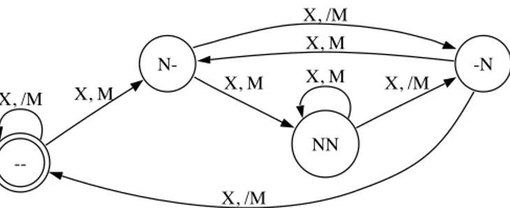
This description leads to generate the 4 states automa-ton shown in figure 3. For each state, the pipeline state is defined at a given time: ’N’ represents an instruction class and ’-’ represents an empty stage. A transition’s condition is composed of an instruction that could be fetched, and the state of the external resource. ’M’ and ’/M’ mean that the external resource is respectively available or busy. An ’X’ for the instruction class or an external resource means that the parameter is irrelevant for the transition’s condition.
The initial state, on the left, represents an empty pipeline. At the next clock cycle, two transitions may be taken. In both transition’s conditions, the instruction class is irrelevant (as there is only one). A transition is taken depending on the state of the external resource. If the resource is busy (transition labelled X,/M), the memory controller access is not allowed and no instruction can be fetched, the pipeline remains in the
--X, /M N-X, M -N X, /M X, M X, /M NN X, M X, M X, /M
Fig. 3. 4 states automaton generated for the very simple example.
same state. If the external resource is available, an instruction of class ’N’ is fetched. The new state of the pipeline is N-.
B. A more realistic example
The second example is more realistic and considers a pipeline with 6 stages. The pipeline is composed of a Fetch stage to get the instruction code in memory, a Decode stage which decodes the instruction, reads operands and performs branch instructions, 2 Execute stages, a Memory access stage and a WriteBack stage that performs write accesses on the register bank. 88 instructions are available in this example.
The concurrency constraints are:
• the registers file is able to perform 3 reads and 2 writes
in parallel;
• an Harvard architecture (separate program and data
mem-ories) is used;
• the computation in the ALU requires 2 stages and is not
pipelined;
Using the HARMLESS ADL, this 6 stages pipeline can be described as follow: architecture Generic { device gpr : GPR { port rs1 : read; port rs2 : read; port rs3 : read; port rd1 : write; port rd2 : write; }
device alu : ALU {
port all;
}
device mem : Memory {
shared port fetch : read;
shared port loadStore : read or write;
}
device fetcher : FETCHER {
port branch : branch;
} }
pipeline pFDEAMWB maps to Generic {
stage Fetch { MEM : fetch;
} stage Decode { fetcher : branch; gpr : rs1, rs2, rs3, rd1, rd2; } stage Execute1 {
alu release in Execute2 : all;
} stage Execute2 { } stage Memory { mem : loadStore; } stage WriteBack { gpr : rd; } }
In the same way, this description declares two objects : architectureand pipeline. In the architecture, many devices are declared. Port loadStore allows the access to 2 methods. the keyword ’or’ is equivalent to the exclusive or. loadStore allows to access the method read or write. At a given time, if an instruction uses read in a stage of pipeline, the second method write becomes inaccessible, and the associated resource is set to busy.
Sometimes, using any method of a component makes it unavailable. Instead of forcing the user to give the list of all methods, an empty list is interpreted as a all methods list. Here the alu device uses this scheme.
When using a port in a pipeline stage, it is implicitly taken at the start of the stage and released at the end. If a port needs to be held for more than one stage, the stage where it is released is explicitly given. Here port all of alu is taken in the Execute1 stage and released in the Execute2 stage.
As in the previous example, shared ports loadStore and fetchare translated to external resources. One is associated with the data memory controller. The other one is associated to the program memory controller. A third external resource is used to check for data dependancies during the simulation (see section III-A2).
Other ports may or may not have an associated internal resource. For instance, the gpr device offers enough ports to satisfy the needs of the instruction set. So no internal resource is used to constrain the accesses to GPR’s methods.
Instruction classes group instructions that use the same resources (internal or external) as presented in section III-B. In this example, 10 resources are used:
• 6 internal resources for the pipeline stages;
• 1 internal resource for the ALU management: alu; • 2 external resources for the memory accesses: fetch
and loadStore;
• 1 external resource to check data dependancies:
dataDep.
As each instruction depends on the fetch resource and the pipeline stages, only three resources can differentiate
instruc-tions: there may be a maximum of 23= 8 instruction classes.
We can notice that an architecture without the ALU structural constraint, the maximum of instruction classes would be reduced to 4. Instructions used in the example (a Fibonacci sequence) are displayed in table I. It uses 5 instruction classes. The 3 remaining instruction classes correspond to impossible configurations.
TABLE I
INSTRUCTIONS USED IN THE EXAMPLE WITH THEXGATE. INSTRUCTIONS THAT USES THE SAME RESOURCES ARE IN THE SAME INSTRUCTION
CLASS.
opcode Alu loadStore dataDep Inst. class
LDW (load) X X 1 STW (store) X X 1 LDH (load) X 2 LDL (load) X 2 MOV X 3 BGT (branch) X 3 BRA (branch) 4 ADDL X X 5 ADD X X 5 CMP X X 5
This example is executed on an Intel Core 2 Duo @ 2.4 GHz processor with 2 GB RAM. The results are the following: 21.3 s are required to compute the whole simulator. This elapsed time is split in 7.7 s to generate the automaton from the pipeline description, 3.1 s to generate C++ files from the automaton and 10.6 s to compile the C++ files (using GCC 4.0). About 30 MB of RAM are required to generate the automaton. The generated automaton has 43 200 states and 325 180 transitions. 2 030 401 pipeline states were calculated and the generated C++ files represent 4.7 MB in 79 800 lines of code. The simulator generation is fast enough to model realistic processors.
VII. SIMULATION RESULT
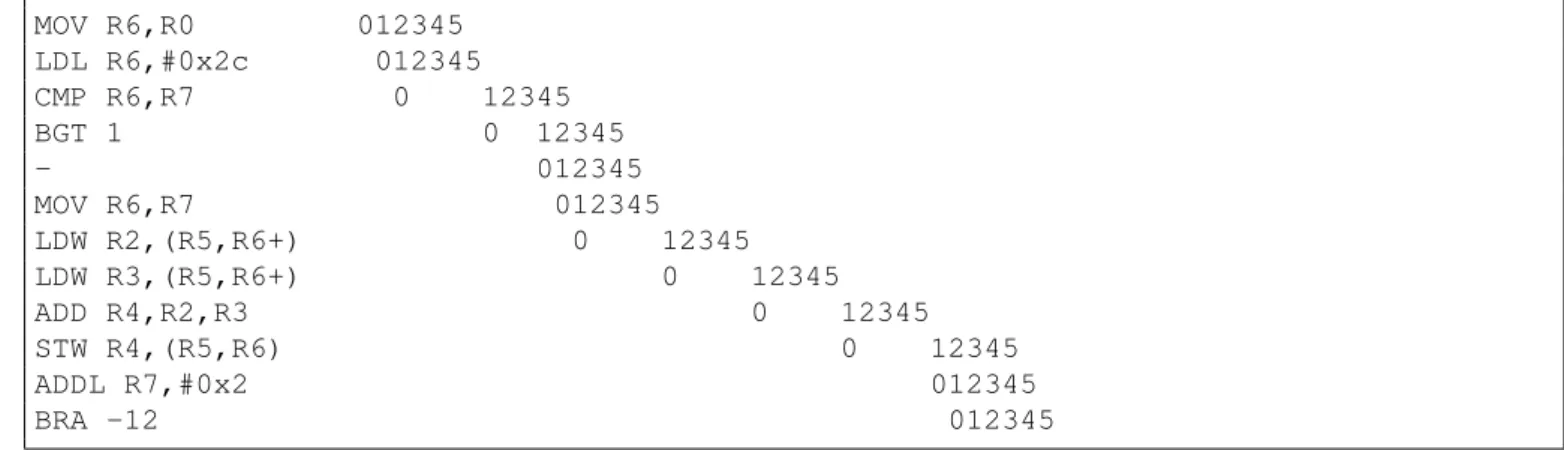
We present in this section the simulation result provided by our tool from the example presented in section VI-B:
• each line represents an instruction that is executed in the
pipeline. The instruction that follows a branch instruction (-) points out that it is a dummy instruction that is fetched before the branch detection in the decode stage (1). No behaviour is associated with the instruction because the branch instruction is taken;
• each column represents one processor cycle. Numbers
from 0 (Fetch) to 5 (Write Back) represent the pipeline stage number in which the instruction is. From this short example, we can get both the functional
behaviour (registers and memory are updated for each in-struction) and the temporal behaviour. This short example of temporal behaviour shows that:
• the four instructions LDW (x2), ADD and STW are data
dependent, and only one instruction is executed at each time in the pipeline. No bypass circuitry is included in our description;
MOV R6,R0 012345 LDL R6,#0x2c 012345 CMP R6,R7 0 12345 BGT 1 0 12345 - 012345 MOV R6,R7 012345 LDW R2,(R5,R6+) 0 12345 LDW R3,(R5,R6+) 0 12345 ADD R4,R2,R3 0 12345 STW R4,(R5,R6) 0 12345 ADDL R7,#0x2 012345 BRA -12 012345
Fig. 4. Execution trace produced by the generated simulator on the Fibonacci sequence
• the BGT instruction (line 4) is delayed for 2 cycles
because it needs the ALU result from the previous instruction (comparison);
The temporal behaviour is required to compute the Worst Case Execution Time (WCET) of real time applications.
VIII. FROM SIMULATION TOWCET
The automaton sequencing is directly linked to the processor clock. Thus, the time required to execute an instruction block depends directly on the number of transitions that are taken during the simulation. This property can be integrated in a static WCET approach, for instance using an Implicit Path Enumeration Technique (IPET) approach [11]. In that case, the simulator has in charge to give the execution time of basic blocks on which the IPET algorithm is based to determine the WCET. Additionally, it can give the pipeline state after the execution of the basic block, directly obtained from the last automaton state. Our tool is being integrated with the OTAWA tool [3]: Otawa is a Framework for Experimenting WCET Computations.
On the real example presented in the previous section, it takes 23.9 s to simulate 100 million instructions (requiring 270 million cycles), on an Intel Core 2 [email protected]. This cycle accurate simulation tool is fast enough to be integrated in such static WCET analysis tools. As a comparison, the Instruction Set Simulator required 6.3 s for the same scenario, but without any temporal information. So the increase factor for computing timing properties is less than 4.
We have focus our study in the pipeline modelling, but other components may significantly influence computation timings, such as caches (branch, instructions or data). Additional delays (that model a cache miss) can be taken into account using external resources, see section III-A2
IX. CONCLUSION
This paper has presented the method used in HARMLESS to generate a Cycle Accurate Simulator from the description of a pipeline and its hazards. The method uses an improved version of the BuildForwardFSA algorithm to handle the data
and control hazards as well as the concurrent accesses to devices that are not managed statically by the automaton. This improvement is done by using external resources at the cost of a larger automaton. The results look promising. By adding cycle-accurate pipeline simulation to an Instruction Set Simulator, the simulation time is only increased by a factor less than 4. Another important part of this work is the design of an Architecture Description Language HARMLESS [7]. A small part of this language is briefly presented here.. It is a very important part because it considerably simplify the design of a simulator - and so the execution time computation - for a particular target processor. Future work will focus on the minimisation of the automaton, the use of multiple automata to reduce the global size of the tables, and to model and simulate superscalar processors. How to model dynamic superscalar processors, including speculative execution is also planned.
REFERENCES
[1] Vasanth Bala and Norman Rubin. Efficient instruction scheduling using finite state automata. In MICRO 28: Proceedings of the 28th
annual international symposium on Microarchitecture, pages 46–56, Los Alamitos, CA, USA, 1995. IEEE Computer Society Press.
[2] Frank Burns, Albert Koelmans, and Alexandre Yakovlev. Wcet analysis of superscalar processors using simulationwith coloured petri nets.
Real-Time Syst., 18(2-3):275–288, 2000.
[3] Hugues Cass´e and Pascal Sainrat. Otawa, a framework for ex-perimenting wcet computations. In European Congress on
Em-bedded Real-Time Software (ERTS), page (electronic medium), ftp://ftp.irit.fr/IRIT/TRACES/6278 ERTS06.pdf, janvier 2006. SEE. 8 pages.
[4] Freescale Semiconductor, Inc. XGATE Block Guide, 2003.
[5] Ashok Halambi, Peter Grun, and al. Expression: A language for architecture exploration through compiler/simulator retargetability. In
European Conference on Design, Automation and Test (DATE), March 1999.
[6] John L. Hennessy and David A. Patterson. Computer Architecture A
Quantitative Approach-Second Edition. Morgan Kaufmann Publishers, Inc., 2001.
[7] R. Kassem, M. Briday, J.-L. B´echennec, G. Savaton, and Y. Trinquet. Instruction set simulator generation using harmless, a new hardware architecture description language. Unpublished.
[8] Kevin Kranen. SystemC 2.0.1 User’s Guide. Synopsys, Inc. [9] J.Y.T. Leung, editor. Handbook of Scheduling. Chapman & Hall, CRC
[10] Xianfeng Li, A. Roychoudhury, T. Mitra, P. Mishra, and Xu Cheng. A retargetable software timing analyzer using architecture description language. In ASP-DAC ’07: Proceedings of the 2007 conference on
Asia South Pacific design automation, pages 396–401, Washington, DC, USA, 2007. IEEE Computer Society.
[11] Yau-Tsun Steven Li and Sharad Malik. Performance analysis of embedded software using implicit path enumeration. In Workshop on
Languages, Compilers, & Tools for Real-Time Systems, pages 88–98, 1995.
[12] Thomas M¨uller. Employing finite automata for resource scheduling. In
MICRO 26: Proceedings of the 26th annual international symposium on Microarchitecture, pages 12–20, Los Alamitos, CA, USA, 1993. IEEE Computer Society Press.
[13] Todd A. Proebsting and Christopher W. Fraser. Detecting pipeline structural hazards quickly. In POPL ’94: Proceedings of the 21st ACM
SIGPLAN-SIGACT symposium on Principles of programming languages, pages 280–286, New York, NY, USA, 1994. ACM Press.
[14] Adriano Tavares, Carlos Couto, Carlos A. Silva, and Jos´e Lima, C. S. Metrˆolho. WCET Prediction for embedded processors using an ADL, chapter II, pages 39–50. Springer Verlag, 2005.