Predicting the Volatility of the Russell 3000 Stock Index

(1)

Predicting the Volatility of the Russell 3000 Stock Index

Bing Xiao1

1_{Management Science, Université d’Auvergne, Auvergne, France}

Correspondence: Bing Xiao, PhD in Management Science, Université d’Auvergne, CRCGM EA 38 49 Université d’Auvergne, Auvergne, France.

Received: March 3, 2016 Accepted: March 19, 2016 Online Published: June 25, 2016 doi:10.5430/ijfr.v7n4p18 URL: http://dx.doi.org/10.5430/ijfr.v7n4p18

Abstract

The forecasting of heteroscedastic models has been a popular subject of research in recent years. The objective of this study is to model and forecast the volatility of the Russell 3000 index during 2000–2015, using various models from the ARCH family. The analysis covers from October 2, 2000 to April 29, 2015 as an in-sample set, and from April 30, 2015 to September 16, 2015 as an out-of-sample set. The measure of the difference between the predicted volatility and the stock’s squared continuously compounded rate of return were estimated by using MAE, MAPE and RMSE. Based on out-of-sample statistical performance, the results reveal that the best estimated model is EGARCH(1,1), and the best model to make dynamic forecasts of volatility is TARCH(1, 1).

Keywords: forecasting, volatility, ARCH, GARCH, GARCH-M, EGARCH, PARCH, TARCH, Hodrick-Prescott Filter, economic cycles, asymmetric effect

1. Introduction

It has become more important for financial institutes to pay attention to the movements of a financial asset. These movements, seen as the risk of the assets, are estimated by the volatility. The non-stationary nature of the series is one of the problems with modelling the volatility. The movements are inconstant, and there are periods with both low and high movements. In 1982, Engle proposed the ARCH model (autoregressive Conditional Heteroscedasticity Model) which was the first model that assumed that volatility is not constant. The ARCH model has been transformed and has led to more sophisticated models, such as GARCH, EGARCH, PARCH and TARCH. In predicting volatility we must ask:Which model captures the volatility better? Could we obtain a more efficient forecast accuracy with a model that better captures volatility? Actually, the results of research in the model’s performance is conflicting and confusing. These observations lead the author to determine how well these different models perform in terms of forecasting. This study focuses on the equity market, It contributes to the existing finance literature by investigating the U.S. stock market during the recent period.

The structure of this article is as follows. Section 2 provides a brief overview of the existing literature. Data and methodology are described in section 3 which recalls the different ARCH Family models. Section 4 displays the results of this study.

2. Literature Review

One of the first studies in conditional variance was the ARCH model proposed by Engle (1982). In his models, the variance of the current error term is assumed to be a function of the actual sizes of the previous time period’s error terms. But Bollerslev (1986) points out the relatively long lag in the conditional variance equation. To avoid problems with negative variance parameter estimates, he proposed the generalization of the ARCH model. To account for the presence of asymmetric effects the EGARCH model was proposed by Nelson (1991). Poon and Granger (2003) noted that due to the negative relationship between volatility and shocks, models that allowed for asymmetric effects were able to provide better forecasts.

For Bracker and Smith (1999), both the GARCH and EGARCH models are optimal for forecasting the volatility of the copper futures market. Carvalho et al. (2006) found evidence of asymmetric effects when using the EGARCH model. Sadorsky (2006) pointed out that there is one type of market that cannot be generalized across other markets as can equity markets and foreign exchange markets which are usually used in volatility modeling. In general stocks with higher kurtosis were better predicted by using the GARCH model, and the EGARCH was better for stocks with lower kurtosis. Ederington and Guan (2004) proposed the GARCH(1,1) model for long memory financial markets, but

(2)

http://ijfr.sci Published by Awrtani an comparison However, n EGARCH predict vola than other m the volatilit and PARC models are 3. Data an The main m 3000 index 3.1 Data The data re we use dat price is the a total of 3 ranging fro 100 observ Figure 1 sh clearly vis non-station stationary w non-norma The summa positive ku of 99%. So and partial iedupress.com y Sciedu Press nd Corradi (200 n of the differe not all the emp

model does no atility exchang models, but no ty of the equity H models wer considered the d Methodolog motive of this p x by using the d equired is the r a on the daily e last trading pr , 903 observati om October 2, vations are treat

hows the Russe ible as well a nary, since its m

with a constant al with fat tails

ary statistics fo urtosis, 0.3007. o, it is mandate autocorrelation I 05) found that ent volatility m pirical studies ot greatly impr ge rates. Marcu ot for a short tim y returns, Accor

e found to be t e best model fo gy

paper is to inve daily data. GAR

eturns on the R price. The req rice of the day. ions. The total 2000 to April ted as an out-o ell 3000 index as the major l mean level is n t mean and vari

and the distrib

Figure 1. Ru or Russell 3000 As per the Jarq ed to convert th n of the Russel International Jou 19 the asymmetr odels, Koksal agree with th rove the foreca

cci (2005) foun me period. Ala

rding to their s the best perfor or the returns s stigate the use RCH, EGARC Russell 3000 in quisite data is o Data on price data set is divi 29, 2015 for m of-sample perio from October long-run rise i

not constant an iance. The outl bution may be a ussell 3000 ind 0 index (Table que-Bera statis he Russell 300 ll 3000 index in urnal of Financia

ric models perf (2009) found t ese findings. R asts. According nd that for a lon am et al. (2013) tudy based on i rming models, series. of ARCH fam CH, PARCH, an

ndex returns ser obtained from t s spans the per ided into in-sam modeling purpo

od in order to a 2000 to Septe in the index i nd rises over t liers (very large asymmetric.

dex and returns A1 in the App stics, Russell 30

0 index series ndicate that the

al Research

form better tha that the EGAR Ramasamy and g to their study ng time period ) studied the us in-sample stati

and all model

mily models for nd TARCH mo ries (Figure 1) the Factset dat riod from Octo mple sets and o oses, a total of assess the forec ember 2015, th in the 2003-20 time. The daily e or very small

s (Daily, 2000 – pendix) reveals

000 index is no into the return e series is non s ISSN 1923-402 an the GARCH RCH(1,1) perfor d Mynisamy (2 y the GARCH the GARCH m se of ARCH m istical performa ls except the G forecasting vo odels are used . In order to ca tabase. The pri ober 2, 2000 to out-of-sample 3,803 observa casts made. he crash of 200 007 and 2008 y return on the l returns) impli – 2015) s a positive ske on-normal at th n series. The pl stationary (Figu Vol. 7, No. 4 23 E-ISSN 192 H(1,1) model. A rmed best. 2012) found th models are be model performs models for forec ance, both the A GARCH and TA

olatility of the R for this study. alculate these r ice taken as th September 16 sets. We use th ations. The rem 00-2003 and 20 -2015. The in e index appear

es that the retu

ewness, 0.9182 he confidence in lotted autocorr ures A1 and A2 4; 2016 23-4031 After a hat the etter to s better casting ARCH ARCH Russell returns, e daily , 2015, he data maining 007 are ndex is s to be urns are 2, and a nterval relation 2 in the

(3)

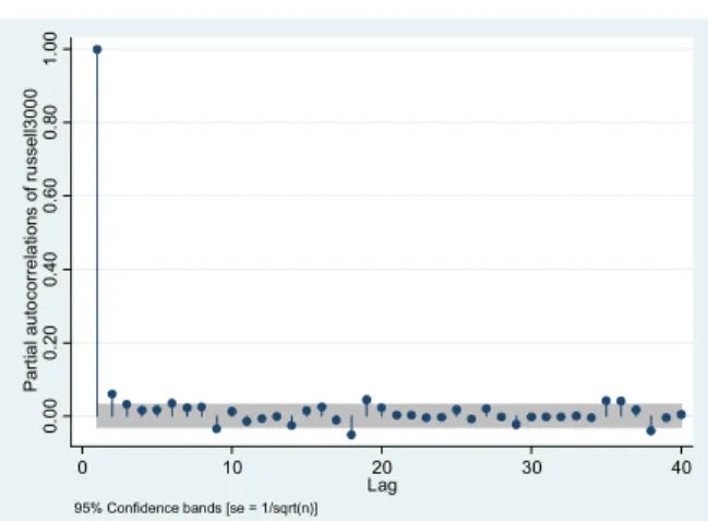
Appendix). Applying the Dickey-Fuller test and the Phillips-Perron test to the series confirms this (Table A2, A3 in the Appendix), and suggests that it cannot be used to model volatility.

In general, the movements of the stock indices series are non-stationary and not appropriate for the study purpose. So, it is mandated to convert the daily price into the return series. The series of the Russell 3000 index is transformed into returns by using the following equation:

= − 1 (1)

Where,

= the rate of return at time t = the price at time t

= the price just prior to the time t

Table 1 summarizes the statistics on returns, showing that the Russell 3000 index have an average daily return of 0.0001833 percent and a standard deviation of 0.01264. The skewness coefficient is –0.03531, its sign being common to most financial time series. The kurtosis value is higher than 3, implying that the returns distribution has fat tails. The ARCH family of models should, therefore, be used to account for these characteristics of the data. It is imperative when modeling such a series that it be stationary and the data mean-reverting. For this purpose, the Dickey-Fuller test is applied to the returns series (Table A4 in the Appendix), and the results show that the series is stationary. On application, the Phillips-Perron test also indicates that the series is stationary and can be used for modeling purposes (Table A5 in the Appendix).

Table 1. Summary statistics for returns

Obs Mean Std. Dev. Min Max Skewness Kurtosis

Returns 3902 0.0001833 0.01264 -0.09280 0.11474 -0.03531 8.38326

The ADF test as well as the PP test are used to get confirmation regarding whether the return series is stationary or not. The values of the ADF test statistic, -68.545, is less than its test critical value, -3.410, at 5%, level of significance which implies that the crude oil price return series is stationary. The findings of the PP test also confirm that the return series is stationary, since the values of the PP test statistic is less than its test critical value. The plotted autocorrelation and partial autocorrelation of squared returns indicate dependence and imply time-varying volatility (Figures A3 and A4 in the Appendix).

3.2 Specification of the Models Used in This Study

To model the volatility of the returns, it is necessary to determine their mean equation. The present returns depend on returns in previous periods. This is the autoregressive component. The residual terms of previous periods are considered the moving order component. To determine the order of the mean equation we plot the autocorrelation and partial autocorrelation of the returns series.

The returns series exhibits “volatility clustering” which is found in most financial time series. This volatility clustering can be seen in Figures A5 and A6 in the Appendix. In order to model behavior such as volatility clustering, the variance of the error term is allowed to depend on its history. Engle’s (1982) classic ARCH model simultaneously models the mean and variance of a series.

3.2.1 ARCH(q) Model

In the ARCH model (Engle 1982) the variance of the current error term is considered to be a function of the actual size of the previous time period’s error terms. The ARCH model is a non-linear model in which the variance does not need to be constant. The error terms are divided into a stochastic component and a time dependent standard deviation :

= (2)

The random variable is a white noise process, and the series is modelled by:

= + + ⋯ + = + ∑ (3)

(4)

http://ijfr.sciedupress.com International Journal of Financial Research Vol. 7, No. 4; 2016

Published by Sciedu Press 21 ISSN 1923-4023 E-ISSN 1923-4031

3.2.2 GARCH(p, q) Model

Bollerslev (1986) and Taylor (1986) generalized the ARCH model which led to their independent development of the GARCH model. The GARCH model is a solution to avoid problems with negative variance parameter estimates using

a fixed lag structure. The GARCH(p, q) model is shown below where p is the order of the GARCH terms and q is

the order of the ARCH terms .

= + + ⋯ + + + ⋯ +

= + ∑ + ∑ (4)

The form of GARCH(1,1) is given below:

= + + (5)

The M in GARCH-M stands for «in the mean». The GARCH-M (1,1) is written as:

= ) + ) + (6)

=

The equation shows that the returns ( ) has a positive relation to its own volatility.

3.2.3 EGARCH Model

The EGARCH model was developed by Nelson (1991). The logarithmic function ensures that the conditional variance is positive and, therefore, the parameters can be allowed to take negative values. The form of EGARCH(1,1) is given below :

log = + log + + | |− 2 (7)

3.2.4 PARCH Model

The PARCH model is a GARCH model with an additional term to account for the asymmetric effect. It employs an indicator function as follows (PARCH(1, 1)):

= + + + (8)

The indicator function takes a value of 1 if the error > 0, and 0 otherwise. For the effect of the previous period’s bad news to be greater than the effect of good news of the same magnitude, γ should be significant and have a negative sign.

3.2.5 TARCH Model

The Threshold GARCH (TARCH) model was proposed by Glosten, Jagannathan and Runkle in 1993 and Zakoian (1994) independently. The coefficients, α and γ, capture the effect of good and bad news respectively. The TARCH model adds a separate variable for negative shocks.

= + ∑ + ∑ + ∑ I (9)

The idea behind TARCH is that it should be better to capture the movements of the negative shocks, due to the fact that they have a bigger effect on the volatility than the positive shocks have.

3.2.6 Asymmetric Effect

The ARCH and GARCH models are easy to identify and estimate. But the symmetric specification is not appropriate if « bad news » has a more noticeable effect on volatility than «good news». This is because their conditional variance which depends only on squared errors is unaffected by the sign of the past period’s errors. We need to test the presence of asymmetric effects before applying the asymmetric models. Engle and Ng (1993) propose various tests to accomplish this. After the GARCH regression, the squared residuals is given by:

= + I + (10)

= 1 when < 0, and 0 otherwise. If the dummy coefficient is significant and positive, this suggests the

presence of asymmetric effects. Then we can determine whether the size of the negative shock also affects the impact on conditional variance by equation (11). For the existence of a size effect, the coefficient must be negative and significant.

(5)

The positive sign bias test determines if the size of a positive shock impacts its conditional variance, the regression is

given by equation (12). For the size effect to be present, the coefficient of and must be

significant.

= + + (12)

3.3 Measures of the Statistical Performance of the Model

After making the forecasts, evaluating them is the next step. For comparison purposes, we compare out-of-sample forecasts with historical volatility. The statistical performance measures, like mean absolute error (MAE); mean absolute percentage error (MAPE); and root mean squared error (RMSE); are applied to pick the best performing model both in the in-sample data set and the out-of-sample data set in this study.

= 1 ∑ | − | (13)

= 1/ ) ∑ | − )/ | (14)

= 1 ∑ − ) ² (15)

4. Empirical Findings (Analysis and Results)

The objective is to determine the performance of these different models in terms of forecasting volatility. In this forecasting approach out-of-sample forecasts are assessed using the last 100 observations of the sample. The study period contains 3, 903 trading days. The in-sample data set covers from October 2, 2000 to April 29, 2015 and includes 3803 observations, whereas the out-of-sample data set covers from April 30, 2015 to September 16, 2015 and incorporates 100 observations.

4.1 Results of Models Estimated

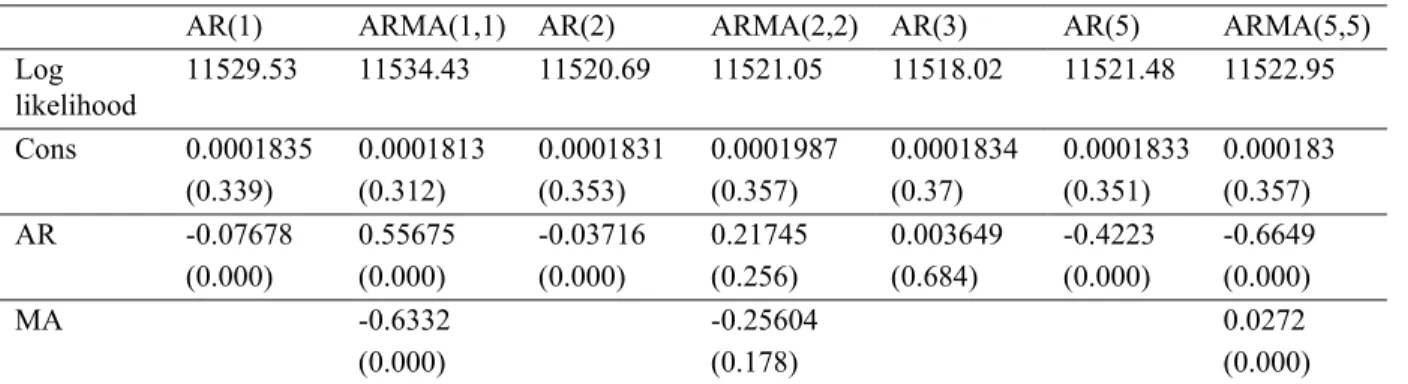
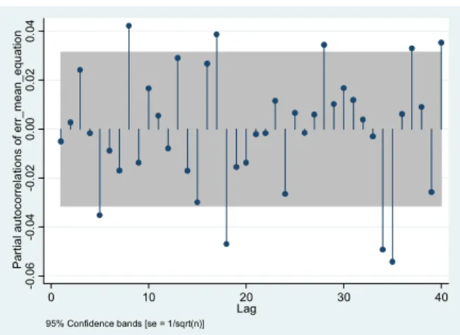
The first step is to identify the mean equation for the returns. The autocorrelation and partial autocorrelation of the returns are significant until the thirtieth lag. An autoregressive moving average ARMA(1, 1) is used as a mean equation to model volatility in the ARCH models. The estimated ARMA(1, 1) equation for the mean is found to be a significant t-value for the coefficients. The residuals of the mean equation indicate the absence of autocorrelation (Figures A7 and A8 in the Appendix).

Table 2. Mean equation estimated

AR(1) ARMA(1,1) AR(2) ARMA(2,2) AR(3) AR(5) ARMA(5,5)

Log likelihood 11529.53 11534.43 11520.69 11521.05 11518.02 11521.48 11522.95 Cons 0.0001835 (0.339) 0.0001813 (0.312) 0.0001831 (0.353) 0.0001987 (0.357) 0.0001834 (0.37) 0.0001833 (0.351) 0.000183 (0.357) AR -0.07678 (0.000) 0.55675 (0.000) -0.03716 (0.000) 0.21745 (0.256) 0.003649 (0.684) -0.4223 (0.000) -0.6649 (0.000) MA -0.6332 (0.000) -0.25604 (0.178) 0.0272 (0.000)

p-values are given in parentheses

There is second-order dependence in the squared residuals of the mean equation and, hence, the presence of conditional heteroscedasticity in the returns (Figures A9 and A10 in the Appendix). Further, the ARCH-Lagrange Multiplier (LM) test confirm the presence of ARCH effects and the need to model this conditional heteroscedasticity using the ARCH family models (Table A6 in the Appendix).

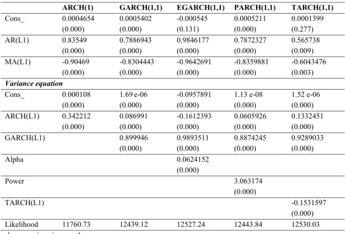
Table 3 presents the results of the models according to the data on returns. The outputs of EGARCH and TARCH on the returns show that the constant is not statistically significant in the mean equation. The ARMA(1, 1) term is also statistically significant for all models. The variance equation illustrates that all the terms are statistically significant at 1% level of significance which implies that the volatility of risk is influenced by past square residual terms. It can be mentioned that the past volatility of the Russell 3000 index returns is significant, influencing the current volatility. The EGARCH variance equation also signifies that the asymmetric effect exists in volatility which means that positive shocks are affecting, volatility differently than negative on volatility.

(6)

We test for the presence of asymmetric effects. The sign bias test yields the following results :

= 0.0001267 + 0.000065 +

p-value (0.000) (0.000)

= 0.0001916 − 0.000065 +

p-value (0.000) (0.000)

The presence of leverage effects are indicated by a positive and significant coefficient which implies the positive and negative shocks have a different effect on the conditional variance. Estimating the negative and positive sign bias tests yields the following results:

= 0.0000988 − 0.0136777 +

p-value (0.000) (0.000)

= 0.0001517 − 0.0018299 +

p-value (0.000) (0.091)

Significant coefficients on both the negative and positive sign bias test implies that there are the sign effects and the size effects. Positive and negative shocks do have a different effect on the conditional variance and their effect on the variance depend on the size of the shocks.

Table 3. Estimated coefficients for the ARCH models

ARCH(1) GARCH(1,1) EGARCH(1,1) PARCH(1,1) TARCH(1,1)

Cons_ 0.0004654 (0.000) 0.0005402 (0.000) -0.000545 (0.131) 0.0005211 (0.000) 0.0001399 (0.277) AR(L1) 0.83549 (0.000) 0.7886943 (0.000) 0.9846177 (0.000) 0.7872327 (0.000) 0.565738 (0.009) MA(L1) -0.90469 (0.000) -0.8304443 (0.000) -0.9642691 (0.000) -0.8359881 (0.000) -0.6043476 (0.003) Variance equation Cons_ 0.000108 (0.000) 1.69 e-06 (0.000) -0.0957891 (0.000) 1.13 e-08 (0.000) 1.52 e-06 (0.000) ARCH(L1) 0.342212 (0.000) 0.086991 (0.000) -0.1612393 (0.000) 0.0605926 (0.000) 0.1332451 (0.000) GARCH(L1) 0.899946 (0.000) 0.9893511 (0.000) 0.8874245 (0.000) 0.9289033 (0.000) Alpha 0.0624152 (0.000) Power 3.063174 (0.000) TARCH(L1) -0.1531597 (0.000) Likelihood 11760.73 12439.12 12527.24 12443.84 12530.03

p-values are given in parentheses.

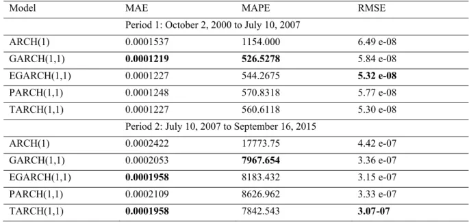
Before making dynamic forecasts of volatility of the Russell 3000 index, the author analyses the statistical performance results of the selected models in the Table 4. The evolution of the Russell 3000 index (see Figure 1) allows us to highlight three identified “peak to peak” cycles during the period from October 2000 to September 2015 (using Hodrick-Prescott Filter). We found two cycles for this period: October 2, 2000 to July 10, 2007 and July 10, 2007 to September 16, 2015. For the first period, it reveals that the GARCH model has the lowest MAE at 0.0001219 and the lowest MAPE at 526.5278. The EGARCH model has the lowest RMSE at 5.32 e-08. For the second period, we

(7)

maintain that the TARCH(1, 1) model is the best model which has the lowest MAE at 0.0001958 and the lowest RMSE at 3.07 e-07. And the same time, the GARCH model has the best MAPE at 7967.654. So, it can be said that all models except the ARCH and PARCH models are nominated as the best model in the case of the Russell 3000 index return series.

Table 4. Statistical performance results for 2 cycles

Model MAE MAPE RMSE Period 1: October 2, 2000 to July 10, 2007

ARCH(1) 0.0001537 1154.000 6.49 e-08

GARCH(1,1) 0.0001219 526.5278 5.84 e-08

EGARCH(1,1) 0.0001227 544.2675 5.32 e-08

PARCH(1,1) 0.0001248 570.8318 5.77 e-08

TARCH(1,1) 0.0001227 560.6118 5.30 e-08

Period 2: July 10, 2007 to September 16, 2015

ARCH(1) 0.0002422 17773.75 4.42 e-07

GARCH(1,1) 0.0002053 7967.654 3.36 e-07

EGARCH(1,1) 0.0001958 8183.432 3.15 e-07

PARCH(1,1) 0.0002109 8626.962 3.33 e-07

TARCH(1,1) 0.0001958 7842.543 3.07 -07

4.2 In-Sample Statistical Performance

The in-sample data set covers from October 2, 2000 to April 29, 2015 and includes 3803 observations, whereas the out-of-sample data set covers from April 30, 2015 to September 16, 2015 and incorporates 100 observations. The following table presents the comparison of the in-sample statistical performance results of the selected models. It reveals that the EGARCH model has the lowest MAE at 0.0002353, the PARCH model has the lowest MAPE at 3910.16 and the lowest RMSE at 6.23 e-07. So, it can be said that, based on the outputs of in-sample statistical performance the EGARCH and the PARCH models are the best models. The TARCH model has the worst MAE, MAPE and RMSE at 0.0004782, 14479.48 and 9.39 e-07 respectively.

Table 5. In-sample statistical performance results

Model MAE MAPE RMSE

ARCH(1) 0.0002410 4757.677 6.49 e-07

GARCH(1,1) 0.0002364 3910.164 6.32 e-07

EGARCH(1,1) 0.0002353 4572.996 6.49 e-07

PARCH(1,1) 0.0002362 3910.159 6.23 e-07

TARCH(1,1) 0.0004782 14479.48 9.39 -07

4.3 Out-of-Sample Statistical Performance

After estimating the models, the next step is to evaluate their forecasts. The next 100 observations the volatility was forecasted by the dynamic models. Two of three evaluation statistics indicate that the TARCH(1, 1) model is best able to forecast volatility. It has the lowest MAPE at 485.6803 and the lowest RMSE at 2.18 e-07. Whereas the EGARCH(1, 1) has the best MAE at 0.0001175. We can constate that there are not a lot of differences between the GARCH model and the PARCH model, but the ARCH(1) has the worst MAPE at 2142.469.

(8)

Table 6. Out of sample statistical performance results

Model MAE MAPE RMSE

ARCH(1) 0.0001428 2142.469 7.45 e-08

GARCH(1,1) 0.0001217 1007.496 7.07 e-08

EGARCH(1,1) 0.0001175 979.8507 6.83 e-08

PARCH(1,1) 0.0001215 1003.461 6.86 e-08

TARCH(1,1) 0.0003036 485.6803 2.18 e-07 5.Conclusion and Discussion

This study has aimed to model the Russell 3000 index return and assess the forecasting ability of the ARCH family of models. We have used historical volatility for modeling through the ARCH family of models and made dynamic forecasts of future volatility. The daily data from October 2, 2000 to September 16, 2015 is used in this study out of which, the in-sample data set covers from October 2, 2000 to April 29, 2015, whereas the out-of-sample data set covers from April 30, 2015 to September 16, 2015.

Based on the results of the in-sample statistical performance, the EGARCH model and PARCH model perform best. Outcomes of the out-of-sample statistical performance demonstrate that the TARCH model and the EGARCH model are considered to be the best model. Those results confirm that the asymmetric effect and the symmetric specification such as ARCH or GARCH are not appropriate in this case. For our study, the best estimated model is EGARCH(1,1), and the best model to make dynamic forecasts of volatility is TARCH(1, 1).

References

Asa Grek. Forecasting accuracy for ARCH models and GARCH(1,1) family – Which model does best capture the volatility of the Swedish stock market?. Spring 2014, Orebro University.

Bollerslev, T. (1986). Generalized autoregressive conditional heteroscedasticity. Journal of Econometrics, 31, 307-327. http://dx.doi.org/10.1016/0304-4076(86)90063-1

Bracker, K., & Smith, K. L. (1999). Detecting and modeling volatility in the copper futures market. Journal of Futures Markets, 19(1), 79–100. http://dx.doi.org/10.1002/(SICI)1096-9934(199902)19:1<79::AID-FUT4>3.0.CO;2-K Carvalho, A. F., da Costa, J. S., & Lopes, J. A. (2006). A systematic modeling strategy for futures markets volatility.

Applied Financial Economics, 16, 819–833. http://dx.doi.org/10.1080/09603100500426408

Ederington, H. L. & Guan, W. (2005). Forecasting volatility. Journal of Futures Markets, 25(5), 465-490. http://dx.doi.org/10.1002/fut.20146

Engle, R. F. (1982). Autoregressive conditional heteroscedasticity with estimates of the variance of United Kingdom inflation. Econometrica, 50, 987–1007. http://dx.doi.org/10.2307/1912773

Goyal, A. (2000). Predictability of Stock Return Volatility from GARCH Models. Retrieved January 2016, from http://www.hec.unil.ch/agoyal/docs/Garch.pdf

Köksal, B. (2009). A Comparison of Conditional Volatility Estimators for the ISE National 100 Index Returns. Journal of Economic and Social Research, 11(2), 1-28.

Marcucci, J. (2005). Forecasting Stock Market Volatility with Regime-Switching GARCH Models. Department of Economics, University of California. San Dieg.

Nelson, D. B. (1991). Conditional heteroscedasticity in asset returns: A new approach, Econometrica, 59, 347–370. http://dx.doi.org/10.2307/2938260

Poon, S.-H., & Granger, C. W. J. (2003). Forecasting volatility in financial markets: A review. Journal of Economic Literature, 41, 478–539. http://dx.doi.org/10.1257/.41.2.478

Ramasamy, R., & Munisamy, S. (2012). Predictive Accuracy of GARCH, GJR and EGARCH Models Select Exchange Rates Application. Global Journal of Management and Business Research, 12(15), 81.

Sadorsky, P. (2006). Modeling and forecasting petroleum futures volatility. Energy Economics, 28, 467–488. http://dx.doi.org/10.1016/j.eneco.2006.04.005

(9)

Tareena Musaddiq. (2012). Modeling and Forecasting the Volatility of Oil Futures Using the ARCH Family Models. The Lahore Journal of Business, 1(1), Summer, 79–108.

Taylor, S. (1986). Modeling financial time series. Chichester, UK: Wiley.

Zahangir Alam, Noman Siddikee, & Masukujjaman. (2013). Forecasting Volatility of Stock Indices with ARCH Model. International Journal of Financial Research, 4(2).

Zakoïan, J.-M. (1994). Threshold heteroscedastic models. Journal of Economic Dynamics and Control, 18, 931–955. http://dx.doi.org/10.1016/0165-1889(94)90039-6

Appendix: Tables

Table A1. Summary statistics for Russell 3000 Index

Obs Mean Std. Dev. Skewness Kurtosis

Russell 3000 3903 1400.60 364.51 0.9182 0.3007

Table A2. Dickey-Fuller test for Russell 3000 index

Test statistic 1% critical value 5% critical value 10% critical value p-value for Z(t)

-0.473 -3.430 -2.860 -2.570 0.8972 Table A3. Phillips-Perron test for Russell 3000 index

Test statistic 1% critical value 5% critical value 10% critical value

Z(rho) -0.449 -20.700 -14.100 -11.300 Z(t) -0.190 -3.430 -2.860 -2.570 MacKinnon approximate p-value for Z(t) = 0.9397

Table A4. Dickey-Fuller test for returns

Test statistic 1% critical value 5% critical value 10% critical value p-value for Z(t)

-67.483 -3.430 -2.860 -2.570 0.0000 Table A5. Phillips-Perron test for returns

Test statistic 1% critical value 5% critical value 10% critical value

Z(rho) -3908.622 -20.700 -14.100 -11.300

Z(t) -68.085 -3.430 -2.860 -2.570

MacKinnon approximate p-value for Z(t) = 0.0000

Table A6. LM test for autoregressive conditional heteroscedasticity

Lags(p) Chi² Df Prob. > Chi²

1 143.203 1 0.0000

(10)

-0 .5 0 0. 00 0. 50 1. 00 A ut oc o rr el at io ns o f r u ss e ll3 0 00 0 10 20 30 40 Lag Bartlett's formula for MA(q) 95% confidence bands

0. 00 0. 20 0. 40 0. 60 0. 80 1. 00 P ar tia l a u to co rr el a tio ns o f ru ss el l30 00 0 10 20 30 40 Lag 95% Confidence bands [se = 1/sqrt(n)]

-0 .1 0 0. 00 0. 10 0. 20 0. 30 0. 40 A ut oc o rr el at io ns of r 2 0 10 20 30 40 Lag Bartlett's formula for MA(q) 95% confidence bands

-0 .2 0 0. 00 0. 20 0. 40 P arti a l a u to co rr e lat io ns o f r2 0 10 20 30 40 Lag 95% Confidence bands [se = 1/sqrt(n)]

-0 .1 0 -0. 05 0. 00 0. 05 Auto co rr el atio ns o f r e tu rn s_ ru ssel l 0 10 20 30 40 Lag Bartlett's formula for MA(q) 95% confidence bands

-0 .1 0 -0 .0 5 0. 00 0. 05 Partia l au to co rre la tio ns o f r e tu rns_ ru sse ll 0 10 20 30 40 Lag 95% Confidence bands [se = 1/sqrt(n)]

Figures

Figure A1. AC of Russell 3000 index Figure A2. PAC of Russell 3000 index

Figure A3. AC of squared returns Figure A4. PAC of squared returns

(11)

-0 .0 6 -0 .0 4 -0 .0 2 0. 00 0. 02 0. 04 Au to co rre la tio ns o f e rr _ m ean _e qu at io n 0 10 20 30 40 Lag Bartlett's formula for MA(q) 95% confidence bands

-0 .0 6 -0 .0 4 -0. 02 0. 00 0. 02 0. 04 P ar tia l au to co rr e la tio ns of e rr _m e an _e qu at io n 0 10 20 30 40 Lag 95% Confidence bands [se = 1/sqrt(n)]

-0 .1 0 0. 00 0. 10 0. 20 0. 30 0. 40 Au to co rr el at io ns o f e rr _ me a n2 0 10 20 30 40 Lag Bartlett's formula for MA(q) 95% confidence bands

-0. 10 0. 00 0. 10 0. 20 0. 30 0. 40 P arti a l a u to co rr e la tio ns o f err_ mea n 2 0 10 20 30 40 Lag 95% Confidence bands [se = 1/sqrt(n)]

Figure A7. AC of res. mean equation Figure A8. PAC of res. mean equation