Algorithmic Intervention to Mitigate Inventory and Ordering Amplification
in Multi-Echelon Supply Chains
By
James Edward Paine
B.S. Chemical Engineering, University of Florida, 2009 M.S. Mechanical Engineering, Georgia Institute of Technology, 2012 M.B.A. Business Analytics and Marketing, Wake Forest University, 2014
SUBMITTED TO THE SLOAN SCHOOL OF MANAGEMENT IN PARTIAL FULFILLMENT OF THE REQUIREMENTS FOR THE DEGREE OF
MASTER OF SCIENCE IN MANAGEMENT RESEARCH AT THE
MASSACHUSETTS INSTITUTE OF TECHNOLOGY SEPTEMBER 2020
©2020 Massachusetts Institute of Technology. All rights reserved.
Signature of Author: ____________________________________________________________________ Department of Management July 30th, 2020
Certified by: __________________________________________________________________________ Hazhir Rahmandad Associate Professor System Dynamics Thesis Supervisor
Certified by: __________________________________________________________________________ David R. Keith Assistant Professor System Dynamics Thesis Supervisor
Accepted by: _________________________________________________________________________ Catherine Tucker Sloan Distinguished Professor of Management Science Faculty Chair, MIT Sloan PhD Program
Algorithmic Intervention to Mitigate Inventory and Ordering Amplification in
Multi-Echelon Supply Chains
by
James Edward Paine
Submitted to the MIT Sloan School of Management on July 30th, 2020 in Partial Fulfillment of the Requirements for the Degree of Master of Science in Management Research.
ABSTRACT
The ‘bullwhip effect’ is a classic, yet persisting, problem with reverberating consequences in inventory management and refers to how forecast errors and safety stock builds yield increasing amplitudes in both orders and on-hand inventory positions the further one moves away from a source of order variability. The bullwhip effect is responsible for both excessive strain on real world inventory management systems, stock outs, and unnecessary capital reservation though safety stock building. In this paper, the author develops algorithmic approaches to mitigating bullwhip using simulation modeling, including cost minimization and amplification minimization, and then interprets the results in the context of existing models of human heuristics in ordering decisions. The algorithmic approaches are optimized as one member within a model of a human decision makers operating within a multi-echelon supply chain with imperfect information sharing and information delays. Within the optimization, human decision biases such as supply line under-weighting are compensated for by the developed methods via the control of the flow of information and simulated physical goods both up and downstream. In all methods developed, inventory and ordering oscillations are minimized in the simulated environment. The overall goal of this project is to develop useful, implementable, and (to the degree possible) understandable algorithms capable of mitigating bullwhip generated by real humans when placed into an actively evolving inventory management crisis in-progress. To this end, the parameters that emerge in the developed algorithm are mapped to previously observed modes of behavior that mitigate the effects of bullwhip. The resulting algorithms act in a manner analogous to those exhibiting high levels of trust within the supply chain, coupled with a cautious approach to information signals outside of the supply chain. Desired stock levels of the resulting algorithms approach those found in optimal base-stock replenishment policies. Finally, it is observed that the algorithm does not fall prey to supply line under-weighting and can act to offset the ordering decisions that typically result in bullwhip in a simulated model of a multi-echelon supply chain.
Thesis Supervisor: Hazhir Rahmandad Title: Associate Professor System Dynamics Thesis Supervisor: David R. Keith
TABLE OF CONTENTS
1. BACKGROUND: THE BULLWHIP EFFECT ... 5
2. METHODS AND MODELING ... 7
Modeling Framework: The Beer Game ... 7
A Discrete Time Model of a Multi-Echelon Supply Chain ... 10
Modeling Human Behavior ... 11
Choice of Cost Function ... 13
Training the ‘Optimized’ Agents ... 14
Baseline Performance and Optimization Choices ... 15
3. RESULTS ... 17
Applications of Trained Optimization to New Order Patterns ... 21
Changing Ordering Behavior During Bullwhip in Progress... 22
4. DISCUSSION ... 27
Interpreting the Parameters ... 28
Caveats and Limitations ... 31
Extensions and Future Work ... 33
5. REFERENCES ... 37
6. APPENDIX ... 40
Model and Code Availability ... 40
Optimization Methods References ... 40
TABLE OF FIGURES
FIGURE 1. EXAMPLE OF BEER GAME BOARD LAYOUT ... 8
FIGURE 2. BASELINE PERFORMANCE: AMPLIFICATION COSTS = 2783.47, INVENTORY COSTS = 3589.96 ... 16
FIGURE 3. INVENTORY COST MINIMIZATION VIA ENTITY 1: INVENTORY COSTS = 2123.92, AMPLIFICATION COSTS = 129.73 ... 18
FIGURE 4. AMPLIFICATION COST MINIMIZED VIA ENTITY 4: INVENTORY COSTS = 7111.23, AMPLIFICATION COSTS = 986.84 ... 19
FIGURE 5. INVENTORY COST MINIMIZED VIA ENTITY 4: INVENTORY COSTS = 3342.22, AMPLIFICATION COSTS = 2144.28... 19
FIGURE 6. COMBINATION OF SEPARATELY TRAINED INVENTORY COST MINIMIZED ENTITIES ... 20
FIGURE 7. BASELINE VERSUS OPTIMIZED ENTITY 1 (RETAILER) RESPONSE TO NOISY ORDERS ... 22
FIGURE 8. SWITCHING FROM BASELINE PARAMETERS TO BOX CONSTRAINT OPTIMIZED PARAMETERS FOR ENTITY 1 AT TIME = 7 ... 24
FIGURE 9. SWITCHING FROM BASELINE TO CONJUGATE GRADIENT OPTIMIZED PARAMETERS FOR ENTITY 3 AT TIME = 9 ... 25
FIGURE 10. SWITCHING FROM BASELINE TO CONJUGATE GRADIENT OPTIMIZED PARAMETERS FOR ENTITY 3 FROM T = 9 TO T = 60 ... 26
FIGURE 11. SUMMARY OF RELEVANT EXISTING RESEARCH IN PERCEPTIONS OF HUMAN VS MACHINE INTERACTIONS ... 34
TABLE OF TABLES TABLE 1. TIME STEP FOR CHANGE IN ORDERING BEHAVIOR ... 23
TABLE 2. EXAMPLE COMPARISON OF STRATEGIES FOR ENTITY 3 AND CONJUGATE GRADIENT OPTIMIZATION ... 27
TABLE 3. RESULTS FOR STEPWISE INCREASE IN DEMAND ... 41
TABLE 4. RESULTS FOR NORMALLY SAMPLED CUSTOMER DEMAND ... 42
1.
Background: The Bullwhip Effect
The field of operations management has increasingly followed its peers in economics, marketing, and finance by endeavoring to recognize the influence of human heuristic-based decision rules and incorporate these behavioral observations into the models of supply chains and inventory management (Gino & Pisano, 2008). Among one of the more studied consequences of behavioral heuristics is the emergence of supply chain instability as embodied by the ‘bullwhip effect’ (Croson et al., 2014). This effect in inventory management is a classic problem with
reverberating consequences though supply chains, both old and modern. Also occasionally referred to as the ‘Forrester Effect’ after Jay Forrester who first formalized the phenomena in his seminal introduction of the field of System Dynamics (Forrester, 1961), bullwhip refers to the increasing amplitudes in both orders and on-hand inventory positions of members of a multi-echelon supply chain the further one moves away from a source of order variability.
The bullwhip effect is responsible for both excessive strain on real world inventory management systems, stock outs, and unnecessary capital reservation though safety stock building (Ellram, 2010). This phenomena is also not necessarily restricted to any one industry, but rather present in varying forms whenever ordering decisions being made in moderately complex and interlinking environments (Lee et al., 2004; Sterman, 1989b, 2000).
Optimal control policies in multi-echelon supply chains are well understood and well-studied. Work by Clark and Scarf demonstrated that an optimal control policy can be applied via a base-stock ordering system when the final customer demand distribution is known (Clark & Scarf, 1960). Their algorithm was later generalized and operationalized to both multi-echelon
supply chains with imperfect local information and stationary demand patterns (Chen, 1999; Chen & Samroengraja, 2009; Lee et al., 2004).
Behavioral causes of ordering and inventory amplification have also been thoroughly explored. A key behavioral bias that leads to bullwhip is commonly identified as ‘supply-chain underweighting’ (Croson & Donohue, 2006; Narayanan & Moritz, 2015; Sterman, 1989a) and emerges as part of a larger anchoring and adjustment heuristic employed by decision makers in an multi-echelon supply chain (Sterman, 1989a; Tversky & Kahneman, 1974). Mitigation of bullwhip has focused on adjusting both the structure of the supply chain itself and the
information availability along the supply chain (Croson et al., 2014; Croson & Donohue, 2006; Wu & Katok, 2006), and on the instruction and training strategies of supply chain managers (Croson et al., 2014; Martin et al., 2004; Wu & Katok, 2006). While mitigation is possible, the underlying ordering heuristics that drive the emergence of bullwhip remain in many of these studies. For many of the above referenced studies, the Beer Game (Sterman, 1989a) is the modeling framework employed to explore and test the interventions developed. The Methods and Modeling section below describes this framework in more detail, but the Beer Game is the original modeling tool used to demonstrate much of the above observations on the origin and nature of bullwhip.
Influence of cognitive features of managers who exhibit greater or lesser degrees of inventory amplification have also been studied (Narayanan & Moritz, 2015). This more recent work operationalizes the concept of supply-chain underweighting in a manner that allows a direct connection between the degree of the supply chain underweighting present in decision making and the degree of inventory and ordering amplification. Most promisingly, this work opens an avenue to create a useful, implementable, and (to the degree possible) understandable
algorithm capable of mitigating bullwhip generated by real humans when placed into an actively evolving inventory management crisis in-progress. More recently, efforts have been made to introduce machine learning and reinforcement methods (Sutton & Barto, 2014) into supply chain management typically using some variant of reinforcement or Q learning (Opex Analytics, 2018; Thompson & Badizadegan, 2015). While these methods have shown immense potential, the research herein implies simpler, more interpretable optimization techniques may be applied to existing models of human decision making in multi-echelon supply chains to achieve bullwhip mitigation without needing to impose any changes on either the system structure (either goods or information flow) or mental models (and corresponding heuristics) in use by managers.
In this manner this work strives to ‘close the loop’ first begun by those endeavoring to define behavioral operations management. In this prior work, the authors define behavioral operations management, in part, by incorporating observations of human decision heuristics into operations management optimization strategies (Gino & Pisano, 2008; Größler et al., 2008). In this paper, by developing methods to minimize cost along a supply chain and mitigate the bullwhip effect, that are also directly interpretable in the context of existing models of human decision making, it is possible to map from optimization routines that minimize cost functions which incorporate the human environment back to interpretable human-modeled decision rules.
2.
Methods and Modeling
Modeling Framework: The Beer Game
To test methods for bullwhip mitigation, an environment is needed. The Beer Game provides an ideal, and well-studied environment. The Beer Game is a classical inventory management and System Dynamics simulation and learning tool, in which a multi-agent decentralized supply
chain is modeled, much like real decentralized inventory management systems). First developed by Jay Forrester at MIT, the game has been used since the 1950’s to illustrate system thinking concepts and the prevalence of the bullwhip effect. Figure 1 below shows the typical starting layout for the game, which is started with 12 units of inventory on hand for each player, and 4 units of inventory in transit at each stage in the shipping system, and 4 orders moving through the order chain. The original purpose of the simulation was to illustrate the difficulty of rational thinking in the midst of time-delayed and non-linear information feedback loops, value of
information sharing, and most classically the bullwhip effect in inventory management (Sterman, 1989a, 1989b).
Following the example of numerous previous studies using this modeling framework (Croson & Donohue, 2006; Narayanan & Moritz, 2015; Sterman, 1989a), the model developed here was also initialized and conceptualized as shown in Figure 1, which also visualizes the typical layout of the tool when used as a board game.
Figure 1. Example of Beer Game Board Layout
Following the same examples from pervious uses of the Beer Game as a model of a multi-echelon supply chain, after four training rounds (where in the customer demand is a fixed quantity of 4 units, and all players are directed to place an order of 4 units downstream), the
customer orders experience a step-wise increase (from 4 units to 8 units per round). From this point onwards, each round of the game proceeds as follows:
1. Receiving inventory and advance shipping delays – Each entity receives the units in the shipping delay immediately to their right. The contents of the furthest shipping delay to the right is moved up
2. Fill orders – Entity 1 (retailer) views the customer order, all others examine the
‘incoming orders’ and orders, inclusive of any outstanding backorders, are filled to the extended inventory allows
3. Record inventory or backlog
4. Advance order slips – the order slips further to the left are moved up
5. Place orders – Each entity decides what to order and places it the ‘orders placed’ box to their right
The stated goal of the game is to reduce the amount of total cost of the entire team, subject to inventory holding costs of $0.50 per units and backorder/stockout costs of $1.00 per unit.
Backorders do not expire under the traditional interpretation of this game and must be filled from existing stock prior to meeting any new demand.
Typically, real human players are placed into this system to make inventory purchasing and management decisions. Within a few rounds of ordering, the bullwhip in inventory and
backorders appears, amplifying over time along the simulated supply chain as each player acts to reserve inventory to satisfy their own myopic forecasts and needs. Exact solutions for optimal ordering quantities have been developed, such as the base-sock method (Chen & Samroengraja, 2009; Clark & Scarf, 1960), but require all agents to be acting rationally and consistently. Additionally, while these optimal ordering methods presume stationary customer order patterns,
which this simulation satisfies, the human participants themselves have no knowledge a priori of the distribution of the customer order pattern.
A Discrete Time Model of a Multi-Echelon Supply Chain
A discrete time model of the Beer Game, following the sequence of steps enumerated above, was created in the R and Pythons scripting languages. This was designed purposefully to mimic the flow of material and information in the same manner as the general description of the Beer Game from the playing of the boardgame described above (Sterman, 1989a). This model was made as both a self-contained simulation of the system over a given time horizon, and as a callable function that takes a given state-action pair and returns an updated state. As this system, and the dynamics it generates, specifically depends on the accumulation of stock variables over time delays, which are in turn a function of the actions taken in all previous realizations of the system, the state variables of the system must contain the current values of all components of the system.
The functionalized form of the simulation was written such that the input state-action pair consists of the current state of all variables and stocks, along with the action of a specific
player/agent in the system given that state. The function then returns the new state of the system given that action. Within this model of a multi-echelon supply chain, a simulation of ‘human-like’ ordering behavior was created, as described the Modeling Human Behavior section below. The functionalized form of the simulation, when applied iteratively, returns the same final state as the full simulation run over the same time horizon. This functionalized form of the Beer Game, combined with the cost functions described in Choice of Cost Function section below, is the testing bed in which subsequent optimizations were conducted for this paper.
Modeling Human Behavior
For the purpose of evaluating a specific machine learning agent or heuristic ruleset within this system, data was obtained from (Sterman, 1989a), (Oroojlooyjadid et al., 2017), and (Martin et al., 2004) on the performance of real human players on the Beer Game, primarily subject to step-changes in customer demand instigating the classic bullwhip effect along the supply chain. The goal of this project is not necessarily to replicate human responses in multi-echelon supply chains per se but rather model the aggregate behavior of the feedback effects of the system when a new optimized entity is introduced.
Therefore, the data collected is used to create a model of how a human would plausibly act given the actions of our machine learning-based agent in the supply chain. The data can be fitted, with reasonable accuracy as shown in both (Sterman, 1989a) and (Martin et al., 2004), to a model of human decision making summarized in expression (1) below:
𝑂𝑡 = 𝑀𝐴𝑋(0, 𝐿̂ + 𝛼𝑡 𝑆(𝑆′− 𝑆𝑡− 𝛽 𝑆𝐿𝑡) + 𝜀𝑡) (1)
𝑤ℎ𝑒𝑟𝑒 𝐿̂ = 𝜃𝐿𝑡 𝑡+ (1 − 𝜃)𝐿̂𝑡−1 (2)
As discussed in the Caveats and Limitations section in more detail below, the choice of decision rule could also have been one that does not presuppose a stationary demand pattern, which is a subtle but nevertheless present assumption in in expressions (1) and (2). Such decision rules have been used in other studies that use the Beer Game as the modeling platform (see for example (Sterman & Dogan, 2015)). However, for this specific project, the data used to create a simulation of plausible human ordering behavior, in which the machine learning methods were trained, was based on a stationary customer demand pattern. Thus, the ordering rule used in expressions (1) and (2) is appropriate for this specific application. The Caveats and Limitations
section provides some additional commentary on this choice and possible extensions to this work.
In expressions (1) and (2) above, O is the order placed at time t given the information observed in the right-hand side of the above expression. In that expression 𝐿̂ is a smoothed interpolation of the expected outflow of inventory, subject to a smoothing parameter θ. SL refers to the total inbound supply line of inventory heading towards the player. S is the current on-hand inventory (or stock), and S’ is a parameter that can be considered analogous to the desired or goal on-hand inventory of the player. Thus, we have an expression with four parameters: θ, α, β, and S’. The data provided allows for fitting of these parameters (based on actual observed order behavior over time, given the current state of the system), at an individual, team (i.e. full supply chain), or even aggregate level. As conceptualized in (Sterman, 1989a), the above parameters are bounded as 0 ≤ θ, α, β ≤ 1 and 0 ≤ S′.
The model of the Beer Game was created here to draw on fitted parameters for any of the above combinations and also ‘bootstrap’ behavior by combining fitted individual parameters into aggregate artificial and ‘human-like’ teams that did not actually exist. This creates a rich and varied environment to test a machine learning algorithm while modeling the feedback effects generated by modeled human behavior.
The value of β specifically maps directly to the degree of supply-chain underweighting, and has been shown in prior work to be directly related to both the cognitive state of the decision maker and ultimately the performance of the supply chain (Narayanan & Moritz, 2015).
Specifically, higher values of β → 1 corresponded to lower reliance on the supply-chain
underweighting, more complete knowledge of the entire supply chain inbound to an entity, and ultimately higher performance in the Beer Game (Narayanan & Moritz, 2015).
Thus, this paper hypothesizes that any optimized agent that minimizes the total costs of the system, as defined in the section below, must have high, if not unity, values of β, when mapped to models of human decision making described above.
Choice of Cost Function
For any optimization, there must be a function or value to optimize over. For this multi-echelon supply chain model, the literal cost is often used to as a performance metric of overall team performance. For example, under the standard configuration of the Beer Game, holding on-hand inventory has a cost of $0.50 per unit per round, whereas backorders (unfilled orders from previous rounds) have a cost of $1.00 per unit per round. Under this costing scenario,
backordered demand never dissipates, and costs continue to accumulate until previously unmet demand is satisfied. This cost rule is summarized in expression (3).
𝐶𝑜𝑠𝑡𝑖𝑛𝑣𝑒𝑛𝑡𝑜𝑟𝑦−𝑏𝑎𝑠𝑒𝑑 = ∑ ∑ (𝐶𝑏𝑜∗ 𝐵𝑎𝑐𝑘𝑜𝑟𝑑𝑒𝑟𝑠𝑡,𝑛+ 𝐶𝑖𝑛𝑣∗ 𝐼𝑛𝑣𝑒𝑛𝑡𝑜𝑟𝑦𝑡,𝑛) 𝑁 𝑒𝑛𝑡𝑖𝑡𝑦=1 𝑇 𝑡=1 (3)
An alternative cost function to consider here is one more closely tied to the original purpose of this project, namely mitigating the bullwhip effect. Responses in the supply chain to step-increases in customer demand are characterized by two sub-phenomena: amplification and phase shift. Under amplification, the maximum order quantity increases further away from the source of the increase (the customer). The phase shift refers to the delay in that amplification occurring in time versus the origin of the signal. Consider a random time horizon T over which the simulation is played, and subject to a step increase in demand of some value. The phase shift is a fixed phenomenon based on information transfer speeds and thus outside the control of our optimized entity (restricting that entity to only have access to its immediate environment, i.e.
non-clairvoyant). Thus, we can consider the amplification seen over the time horizon T by any entity in the supply chain as our cost function to minimize. The exact nature of penalizing this amplification can vary, but for this project this cost was chosen as cumulative over the entire horizon T and entities n (as opposed to just considering the point maximum amplification over T). For this paper, this amplification cost function is formulated as seen in expression (4).
𝐶𝑜𝑠𝑡𝑎𝑚𝑝𝑙𝑖𝑓𝑖𝑐𝑎𝑡𝑖𝑜𝑛−𝑏𝑎𝑠𝑒𝑑 = ∑ { ∑ [𝛾 (𝑂𝑟𝑑𝑒𝑟𝑠𝑡,𝑛− 𝐶𝑢𝑠𝑡𝑜𝑚𝑒𝑟𝑂𝑟𝑑𝑒𝑟𝑠𝑡 𝐶𝑢𝑠𝑡𝑜𝑚𝑒𝑟𝑂𝑟𝑑𝑒𝑟𝑠𝑡 ) 2 + 𝜓] 𝑁 𝑒𝑛𝑡𝑖𝑡𝑖𝑒𝑠=1 } 𝑇 𝑡=1 (4)
In the above expression, γ and ψ can be used to scale the penalization with respect to the degree of amplification. The above functional form was chosen purposefully to smoothly approach its maximum value (to aid in the convex optimization described below), and non-linearly penalize larger amplitudes.
Training the ‘Optimized’ Agents
An important note concerns the definition of ‘optimality’ as used in this paper. Here, this refers to the combination of parameters values, bounded by the physically feasible space, that are cost reducing when applied to a given entity in this supply chain (with all other entities modeled as make simulated ‘human-like’ ordering decisions).
One of the goals of this paper is to ultimately create an interpretable trained entity whose decision-making parameters can be translated towards human learning. It should be noted that the term ‘optimal’ here, when used, is referring to an agent that minimizes supply chain costs, as defined by either expressions (3) or (4) above, given that the other agents in the supply chain exhibit ‘human-like’ ordering behavior. This definition of optimality purposely does not refer to
previously identified optimal control polices like those of (Clark & Scarf, 1960), which assume fully rational decision making for all entities in the supply chain that furthermore have
knowledge that the customer order pattern is stationary.
Originally, an Actor-Critic Policy Gradient method was originally pursued to train the optimized entity and explore the resulting behavior. However, considering the goal of
interpretability, this project instead focuses on the results of optimizing the above costs functions with respect to expression (1) directly. To this end, expression (1) was optimized relative to both cost functions show in in expressions (3) and (4), and with varying the position of the optimized entity between 1 (the ‘retailer’) and 4 (the ‘factory’) as shown in Figure 1. To test robustness, the parameters for the other simulated players where drawn from a variety of combinations of
available values as discussed in the Modeling Human Behavior section above. However, the general results are the similar independent of the choice of parameters from the feasible (and previously fitted from real data) set. Therefore, the results below are shown relative to the ‘general’ case set of parameters, i.e. the average parameter values that show typical human responses in this environment (again refer to (Sterman, 1989a)).
Baseline Performance and Optimization Choices
As stated above, the below are selected results for specific parameter values, however the general observations still hold under other choices. For optimization over the cost function shown in expression (4), ψ and γ were chosen as +25 and +1 respectively, simply for convenience of scaling the typical output of this function to the same order of magnitude as that generated by expression (3).
For expression (1), simulated ‘human-like’ entities in the supply chain responding to the
optimized agents had parameter values of θ = 0.36, α = 0.26, β = 0.34, and S’ = 17, which come from aggregates of the fitted behavioral data from (Sterman, 1989a), directionally confirmed by a similar analysis in (Oroojlooyjadid et al., 2017).
Additionally, while the game is traditionally run over 36 rounds, the simulations below are over 104 rounds to give time for amplification to fully develop and dissipate. Figure 2 below shows the ordering behavior of the baseline case, with the default human-like agents responding to a step change in customer orders, along with the costs incurred from expressions (3) and (4).
Figure 2. Baseline Performance: Amplification Costs = 2783.47, Inventory Costs = 3589.96
As summarized in Table 3 and Table 4 in the Appendix, several different numerical optimization methods (Bertsimas & Tsitsiklis, 1997) were tested across each entity position in this simulated supply chain. As discussed in the Modeling Human Behavior section above, the parameter space is four dimensional and bounded as θ ∈ ℝ+, 0 ≤ α ≤ 1, 0 ≤ β ≤ 1 and 0 ≤ S′.
Previous analyses of optimal decision rules in models of multi-echelon supply chains like the Beer Game have either assumed or proved convexity of the underlying cost function (Chen, 1999; Clark & Scarf, 1960). While such a proof of convexity of the system as modeled here,
incorporating the behavioral heuristics of equation (1) into (3) or equation (4), is beyond the scope of this paper, it allows us to narrow optimization strategies to a class of bounded and convex or pseudo convex optimization methods.
Fortunately, as seen by inspection of Table 3 and Table 4 in the Appendix, choice of convex optimization method ultimately generated qualitatively similar results, as did the choice of cost function, shown in expressions (3) and (4). To further build confidence that the
optimization routine returned a local minimum of the overall system cost, a bounded axial search (Nash et al., 2020) along the four parameters was conducted after each minimization and no significant reduction in system cost was found. Thus, while the results given below may be framed in the context of a single observations, they are generally valid along all observations derived for this paper, unless stated otherwise.
3.
Results
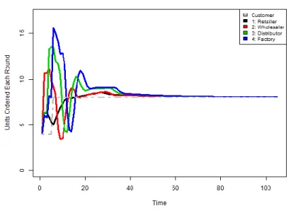
Figure 3 below shows the general trend when optimizing for a minimum cost, i.e. via equation (3). Here the example is an optimization along Entity 1, or the Retailer as shown in Figure 1. The optimization quickly produces damped system, eliminating oscillations and amplification. But it does so at the cost of backorders, essentially driving the on-hand inventory of the optimized entity to zero and incurring backorder costs for at least some portion of the simulation.
Figure 3. Inventory Cost Minimization via Entity 1: Inventory Costs = 2123.92, Amplification Costs = 129.73
By visual inspection of the simulation results, and as summarized in Table 3, the
inventory cost minimization method is generally superior at minimizing both the costs incurred to the supply chain as defined in expression (3) and simultaneously reduce the amplification costs as defined in (4). While minimizing along equation (4) did consistently reduce
amplification relative to the baseline shown in Figure 2, it did so sometimes at the cost of enduring high levels costly of backlog. As an example, consider the task of optimizing the behavior of Entity 4, or the Factory, given that all upstream players are modeled as ‘human-like’. As seen in Figure 4 below, optimizing for amplification reduction, i.e. equation (4), does in fact reduce the amplitude in orders experienced by the supply chain in net, but does so by incurring comparatively massive backlogs in the Factory.
Figure 4. Amplification Cost Minimized via Entity 4: Inventory Costs = 7111.23, Amplification Costs = 986.84
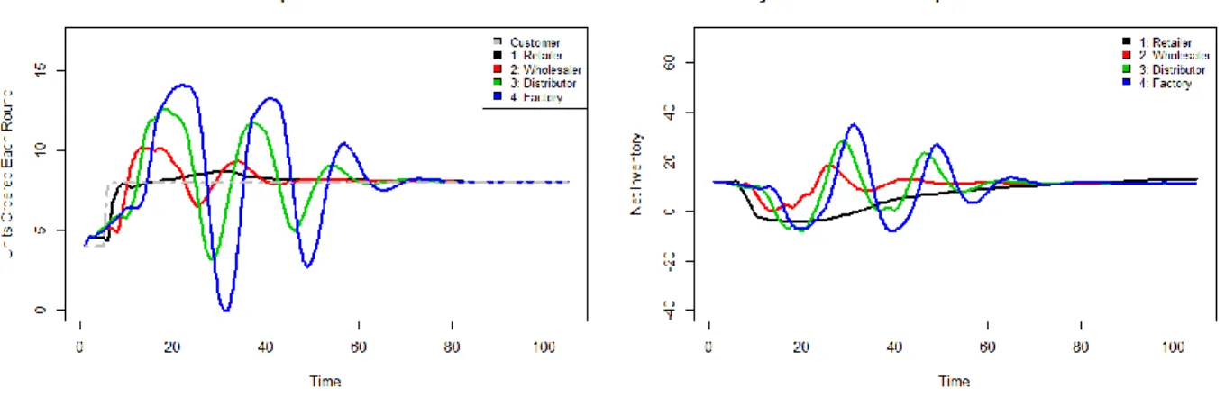
Whereas minimizing along inventory costs, i.e. equation (3), attempts to balance the amplification damping benefit of backlogs with the incurred cost of sustaining an ever-increasing backlog. As seen in Figure 5, the reduction to amplification is less than discussed above, but still present while the runaway costs are avoided.
Figure 5. Inventory Cost Minimized via Entity 4: Inventory Costs = 3342.22, Amplification Costs = 2144.28
The above minimizations of cost were optimized one entity at a time, under a model that assumes that all other entities in this simulated supply chain order in a ‘human-like’ manner. The hypothesis and background introduced at the start of this paper presume that a lessening of supply-chain underweighting and generally behavior that resembles both high cognitive
reasoning individuals, and also teams of such individuals, like that shown in (Narayanan & Moritz, 2015) will mitigate bullwhip.
To explore this and test if the optimized parameters space found by the above cost
minimizations work not only in isolation, but also in conjunction, consider the behavior shown in Figure 6 below. Here is an example of all four trained agents interacting with each other in the simulated supply chain. Each entity was trained separately, exposed to simulated ‘human-like’ ordering behavior from the rest of the supply chain. While Figure 6 represents a single example of combining all four trained agents together, the outcome is similar in all the optimization combinations performed, as seen in Table 3 and Table 4. The amplification in orders is rapidly damped in this simulation, achieving the goal of bullwhip reduction in a manner that implies robustness towards applying each separately trained agent towards and an environment with fundamentally different ordering heuristics than that in which it was trained.
Applications of Trained Optimization to New Order Patterns
Perhaps more surprising and reassuring about the general application of the results of this project, is the application of the optimized agents to a different customer order string. The parameters that minimize total team cost, weather actual inventory cost or amplification costs, were trained on the step-wise increase of the traditional Beer Game, but then applied to a
scenario where customer orders are drawn from a normally distributed random variable (Table 4 in the Appendix for detailed results for each scenario).
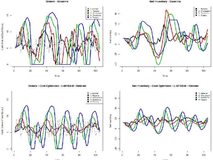
As seen in Figure 7, again showing only one representative example, the optimization function trained on a step-wise increase in customer demand still reduces both cost functions relative to the baseline performance of all simulated human-like players.
Inspection of Table 3Table 4 does shows similar points of caution as seen in the base optimization case discussed above. Namely, that minimizing towards amplification costs often does so at the detriment of the overall incurred backlog cost of the system. However, this result indicates that the parameters found in the above described minimizations are not only capable of reducing the costs incurred in this simulated multi-echelon supply chain subject to the training customer order string, but are generally capable of reducing bullwhip.
Figure 7. Baseline versus Optimized Entity 1 (Retailer) response to noisy orders
Baseline: Inventory Costs = 4350.79, Amplification Costs = 11988.70 Optimized: Inventory Costs 2968.90, Amplification Costs = 6178.59
Changing Ordering Behavior During Bullwhip in Progress
To further explore the generality of the above derived optimization to a wider class of order stings, consider the an entity in this multi-echelon supply chain acting in a manner consistent with the Baseline behavior seen in Figure 2, and parameterized per the first line of Table 3 (with θ = 0.36, α = 0.26, β = 0.34, and S' = 17). The above analyses assume that these parameters can be replaced with their optimized values prior to the emergence of any inventory or ordering amplification. However, it is conceivable that an entity in this supply chain may be able to
change their ordering method once they become aware of the emergence of an actively evolving inventory management crisis in-progress, as encapsulated by the bullwhip effect.
By inspection of the ordering history of the baseline scenario shown in Figure 2, there are three possible moments an entity in this supply chain could possibly recognize the existence of ordering amplification:
1. At the maximum of one of its own spikes in ordering behavior
2. When the orders of an upstream entity surpass its own (i.e., for the ‘retailer’ in position 1, this would be the ‘warehouse’ in position 2)
3. When the orders of a downstream entity surpass its own (i.e., for the ‘factory’ in position 4, this would be the ‘distributor’ in position 3).
The exact ability of each entity to observe this information may be limited by the structure of the supply chain itself, and very possibly could be under the same information delays modeled in order transmittal system. However, for ease of analysis and generality of results this specific delay is ignored.
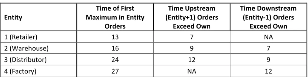
By inspection of the data that underlies Figure 2, the time steps that each of the above three scenarios was chosen for further analysis and is summarized in Table 1 below.
Table 1. Time Step for Change in Ordering Behavior
Entity Time of First Maximum in Entity Orders Time Upstream (Entity+1) Orders Exceed Own Time Downstream (Entity-1) Orders Exceed Own 1 (Retailer) 13 7 NA 2 (Warehouse) 16 9 7 3 (Distributor) 24 12 9 4 (Factory) 27 NA 12
As an example to help read Table 1, in the first entity (the retailer) would change from the default ordering parametrization (θ = 0.36, α = 0.26, β = 0.34, and S' = 17) to a previously determined optimized set of parameters (such as the BOBYQA inventory cost minimizing values of θ = 0.037, α = 0.126, β = 0.903, and S' = 36) at a time of t = 7 if it was changing its ordering behavior once it notices upstream orders exceeding its own.
Figure 8 below shows a representative example of the ordering and inventory behavior across the system when the ordering parameters for the first entity (the retailer) are switched from the baseline values to those found in the previous optimization under the box constraint method using the inventory based cost function from equation (3). Values for both the resulting inventory based and amplification-based costs that are occurred across the system, using all permutations of the times shown in Table 1, are given in the Appendix in Table 5.
Figure 8. Switching from Baseline Parameters to Box Constraint Optimized Parameters for Entity 1 at Time = 7
Inspection of the values in Table 5 yields an interesting observation. Aside from the position of the retailer (Entity 1), changing ordering behavior in response to the emergence of bullwhip yields higher inventory-based costs in net versus if the entity had simply stayed with the default parameterization. However, amplification-based costs are consistently and
dramatically reduced versus the baseline. This observation is consistent no matter if expression (3) or (4) was used to train the agent. Figure 9 below provides some insight on the source of this seeming paradoxical observation. Here we see the source of the long-term inventory costs as the entity continues to hold larger amounts of inventory that necessary later into the simulation. However, overall ordering amplification is tamped down quickly by this action and allows for bullwhip as defined at the beginning of this paper, to be halted quickly after it is first observed.
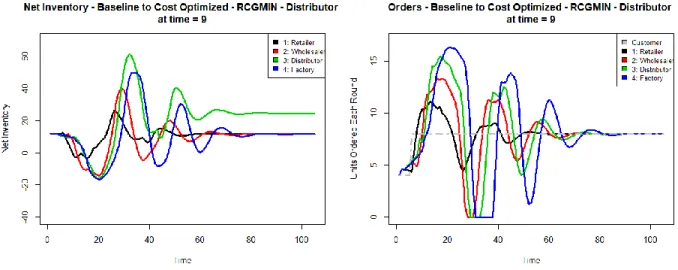
Figure 9. Switching from Baseline to Conjugate Gradient Optimized Parameters for Entity 3 at Time = 9
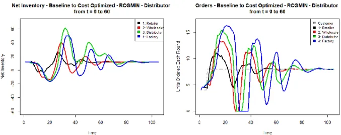
An argument could be made that an entity willing to switch ordering behavior at the onset of suspecting bullwhip in the supply chain may be willing to do so again once that bullwhip as subsided. The same scenario as shown in Figure 9 above (entity 3, the wholesaler, switching from the baseline ordering behavior to those determined under the box constraint optimization method when the first downstream order exceeded its own, at a time step equal to 9), can be compared to one in which this same entity switches back to the baseline ordering behavior after the bullwhip has passed. Arbitrarily choosing a time step of t = 60 as a sufficiently far in the future gives the results in Figure 10 below. Utilizing this strategy of changing ordering behavior in the presence of bullwhip, but then changing back to the default behavior helps mitigate the
effects of inventory and ordering amplification during the event, but then allows the entity to return to typical stock levels afterwards.
Figure 10. Switching from Baseline to Conjugate Gradient Optimized Parameters for Entity 3 from t = 9 to t = 60
Unsurprisingly, this switching of ordering behavior yields results that lie in between those seen using optimized ordering parameters for the entire time horizon (as seen in Table 3) and switching from the baseline during the bullwhip and maintaining this new value for the entire time horizon (as seen in Table 5). Rather than do a point-by-point comparison across all combinations of optimization methods and possible order strategy switching times, Table 2 below provides numerical results from the example explored immediately above, focusing on entity 3 (the distributor) under a conjugate gradient optimization scheme.
These observations reinforce two key points: 1) That either choice of optimization method (inventory costs centric or amplification centric) has similar results in reducing amplification-based bullwhip in this multi-echelon supply chain and 2) that when considering what is successful mitigation of bullwhip one must consider both the definition of costs and the underlying problem itself as separate yet still coupled problems.
Table 2. Example Comparison of Strategies for Entity 3 and Conjugate Gradient Optimization
Scenario Description Time Period Total Team Cost (Inventory-Based)
Total Team Cost
(Amplification-Based)
Baseline NA 3589.96 2783.47
Optimized ordering parameters
from the beginning Full horizon (t>0) 3180.47 (-11.41%) 1029.78 (-63.0%) Switch to optimized parameters
when downstream (Entity-1) orders exceed own
t ≥ 9 3353.59 (-6.58%) 1482.25 (-46.75%)
Switch to optimized parameters when downstream (Entity-1) orders exceed own and switch back after bullwhip has passed
9 ≤ t ≤ 60 3090.84 (-13.9%) 1533.65 (-44.9%)
4.
Discussion
The above results emphasize that it is important to remember the context in which any cost minimization activity occurs. While the stated purpose of this paper is to investigate algorithmic interventions to reduce bullwhip, which is generally defined in terms of signal amplification, the costs of those interventions must be considered and weighed. The results presented above comparing the results of minimizing on total system inventory cost versus total system amplification illustrate the tradeoff. Specifically, the tradeoff between the damping value of incurring backlog and the cumulative cost of such a decision is captured best when it is priced, and when that price is incorporated into the minimization exercise.
However, when choosing a cost function that does represent the underlying structure and cost tradeoffs of the system, it is possible to construct an algorithmic intervention that acts on only one entity, or multiple entities, in the Beer Game that:
1. Reduce cost, measured both in terms of inventory and backorder costs and amplification, relative to a baseline of an all-human team
2. Does so without imposing any additional constraints on the behavioral ordering of the human partners in the system.
Stated differently, the above optimization has shown that it is possible to let people be people and continue to exhibit the behavioral ordering heuristics observed for more than 60 years, while still mitigating bullwhip in supply chains. For more insight on how this algorithmic intervention maps to existing models of ordering decision making, we must investigate the parameters that minimized the cost functions in the above described optimization exercise.
Interpreting the Parameters
The above observations of the ability of our optimized agents to mitigate bullwhip in a multi-echelon supply chain, while allowing all other human-like decision makers in the supply chain to continue to act like humans (i.e., still exhibit supply chain underweighting), can now be
inspected in more detail. By inspection of expression (1), expression (2) and the detailed results in Table 3, the following main observations about parameter space of the optimized entities can be made:
• Low values of θ for the Retailer and high values of θ for everyone else:
This parameter determines the degree of smoothing in updating each entity’s expectation of future orders in the same manner as the classic anchoring and adjustment heuristic (Tversky & Kahneman, 1974). For low values of θ, the entity is slow to update expectations while for high values of θ, the entity is quick to adopt the new order signal being received as their expectation for the future. Here,
low values of θ for the Retailer, or Entity 1, means that this entity which is most downstream in the chain and most influential towards information flow upstream to other supply chain partners, is slow to update their expectation of changes in customer orders and thus unlikely to rapidly change order signals. Conversely, the high (often at or near 1) values of θ for downstream entities can be interpreted as a high level of trust in the order signals being sent from upstream partners. As discussed in prior research, trust is an essential part of a well-functioning supply chain and some degree of trustworthiness must be assumed in a well function integrated supply chain (Özer et al., 2011). The values of θ found here imply that bullwhip minimization is achieved, in part, by cautious response to changes in order signals from customers, but full trust in order signals from partners. • Very high values of β at all positions in the supply chain:
As hypothesized in the Methods section above, all entities optimized to minimize the cost of the system in the presence of simulated human-like partners did so in part by not falling prey to the supply chain underweighting heuristic observed in previous empirically-grounded work (Narayanan & Moritz, 2015; Sterman, 1989a). As the value of β approaches 1, the decision rule shown in equations (1) and (2) begin to consider the entire inbound supply line with no or minimal discounting. Differing values of this parameter were used in previous studies to show how different levels of cognition in real human players of the Beer Game resulted in differing levels of inventory and ordering amplification.
Correspondingly, the entities developed here, optimized to minimize system costs in the presence of human-like supply chain partners, act like the high cognition
players seen in those previous studies (Narayanan & Moritz, 2015) by completely considering the inbound supply line when making ordering decisions.
• Values of S’ resembling a base-sock replenishment method:
The parameter S’ maps approximately to the level of inventory on hand that the decision maker strives to maintain. Of interest, the values of S’ arrived at by the optimized entities generally match a policy resembling a base-stock order method as expected in a full-information system with full rational entities (Clark & Scarf, 1960). The above optimization varies S’ and α to create an effective base-stock level that minimizes the total cost of the system. For example, in the long-run steady state under the traditional customer order string of stepping from 4 to 8 units, and a balanced information and delivery day of 2 time periods each, we can expect a total of 16 units to be on-order in total (8 for each unit of time) and correspondingly 16 units in transit. Together, this represents 36 units that can be expected to flow into the on-hand inventory of the entity. Assuming incoming orders remain stable at 8 and outgoing orders match that number then maintaining a base-stock level of 36 is a realistic simplification of the full optimal policy. Inspection of Table 3 shows that for the great majority of the optimizations performed, the value of S’ that minimized costs along the entire supply chain was found to be at or near 36. Significant deviations from this value occurred only in Entity 3, the Wholesaler, which maintained a larger base stock level. Given that this position is also the one that typically experienced the least minimization in costs, increased safety stock to offset higher variability both incoming and orders and incoming supply is to be expected.
Caveats and Limitations
A notable caveat exists to the discussion above about the applicability of the parameters to novel customer order patterns. As seen by inspecting the randomly drawn customer order string
illustrated in Figure 7, and explicitly stated in the description of Table 4, this randomly drawn order string is still stationary (centered around a demand of 6 units per time period with a standard deviation of 2 units per time period).
As discussed in more detail in the Interpreting the Parameters section above, the optimized parameter S’ determined under the step function converge to what is effectively a base-stock policy value. The random signal used above is centered and stationary in, roughly, the same range as the step change signal used to train the agents and thus the value of S’ is expected to work in both scenarios. When the demand pattern become stationary, or when the mean of the new pattern varies significantly from that used in the training set, then one would expect
optimized parameters to work less well. As discussed in other related works (perhaps most notably (Sterman & Dogan, 2015)), the optimal value of S’ given a foreknowledge of a
stationary demand pattern, and full weighting of the supply line (i.e. a value of 𝛽 = 1) reduces to the classic base-stock ordering rule (Clark & Scarf, 1960) in similar contexts have been
described in other works. As discussed in the Interpreting the Parameters section above, the optimization used here does approach this rule but does not quite align perfectly with it. Because the agent developed here exists in the middle of a larger supply chain (with the exception of the role of ‘Retailer’), it is not necessarily exposed to a truly non-stationary demand signal from the human-modeled simulation in which it exists. However, the input demand signal from the ‘customer’ is stationary as implemented here (after the initial step-change).
Thus, it could be argued that the exact parameters developed in this work are only truly applicable to the format of the simulation used to derive those parameters. Specifically, that the stationarity of the input customer string, and the specific design choices of shipping and
information delay times, drive the optimized values of S’.
This caveat does imply that direct application of the specific parameters seen in Table 3 and Table 4 (most notably S’) to an arbitrary supply chain is not appropriate nor robust. This observation does not, however, reduce the generality nor the validity of the observations made in the Interpreting the Parameters section above. Inspection of the parameter values in Table 3 and Table 4, and as discussed above, do show differences by both the definition of cost function and by position in the supply chain. That these differences are anchored to the expected optimal value seen in base-stock level reordering, but adjusted by the location in the supply chain (and thus the degree of uncertainty in the underlying assumptions of stationarity in the base-stock reorder policy), lends weight to the more general observations in the Interpreting the Parameters section above.
It does imply that there is room for future work in this space, by determining a more general, but still interpretable, algorithmic intervention when the input demand is expected to nonstationary. A limitation of this study is that the underlying human-based dataset which was used to construct the simulation in which the optimization was conducted is drawn from prior studies that use stationary customer demand patterns (specifically (Sterman, 1989a)). Thus, while incorporating a more general decision rule seen in expressions (1) and (2), would perhaps allow for further cost reduction and wider application of the derived parameters to scenarios beyond that used here, the core observations of this study would remain intact.
Extensions and Future Work
While the above analysis and discussion is hopeful towards achieving the stated goal of creating an understandable algorithm capable of mitigating bullwhip, it remains to be seen how useful and implementable the above methods are until placed in the context of actively evolving inventory management crisis in-progress, as encapsulated by the bullwhip effect, generated by real humans. Therefore, the next phase of this project will be the incorporation of one of the developed cost minimization algorithms into a real session of the Beer Game.
It is hoped that this future empirical study will not only lend external validity to the observations made in this paper but also shed additional light on confounding variables from human/machine interactions. Specifically, prior work on human/machine interactions provides conflicting conclusions, with some implying that people treat machines like people (Reeves & Nass, 1998), while others imply people behave differently when communicating with a machine than with another person (Shechtman & Horowitz, 2003). The difference between these two conclusions may have material influence on the results of any empirical study of the
interventions described in this paper. This implies the need for full two-by-two empirically grounded test of the optimizations and observations of this paper interacted with the perception of the optimization as being a machine or a human player. Figure 11 summarizes some of the existing research relevant to testing both the empirical applicability of the work of this paper in the context of the Beer Game, and the interacting effect of perception of human versus computer players.
Figure 11. Summary of Relevant Existing Research in Perceptions of Human vs Machine Interactions
In Figure 11, the upper left-hand quadrant (Human-Human) encompasses the vast
majority of existing research in ordering behavior in multi-echelon supply chains, using the Beer Game as an empirical testing and observation tool. Much of the material described and cited in the Background section at the start of this paper falls into this portion of Figure 11. The opposing lower right-hand quadrant (Machine-Machine) is the direct application of the conclusions of this paper to a run of the Beer Game with real players corresponds to the. Here a single member of the simulated multi-echelon supply chain would be replaced with an ordering rule that utilizes one set of the optimized parameters found in this work, with the real human players being made fully aware of this substitution. These two quadrants correspond to a proposed ‘phase 1’
empirical test and extension of this paper, wherein the performance of the proposed optimization is tested in the context of real human ordering.
While, these observations and conclusions drawn above come from the use of well-known optimization methods mapped to a model of human ordering behavior, real human ordering behavior may be significantly more complex than that simulated above, and could require a more robust algorithmic intervention in order to respond appropriately to orders
generated from real humans in any future empirical study. Based on the various tests performed under differing order strings, both random and step, in the Results section, and the examination of the optimized ordering rules in the Discussion section, I hypothesize that this relatively simple set of ordering rules will still reduce inventory and ordering amplification when placed in the midst of real human ordering. However, this can be tested and is the next step of this research. However, to address this concern more fully, more complex optimization methods are under development (like a proposed Actor-Critic Policy Gradient optimization), which could be more applicable to real-world settings. Furthermore, such a system could perhaps escape some of the caveats and limitations presented immediately above, most notably being more robust to nonstationary customer order signals.
However concerns remain about the interpretability of such a solution, and indeed if it would be necessary in light of the mapping between the optimizations seen in this paper and previous work on high cognitive individuals (Narayanan & Moritz, 2015). The tradeoff between robustness of such an algorithmic intervention with its interpretability and comparative utility remains the focus of future research.
The remaining two spaces in the off-diagonal of Figure 11 propose exploring the effect of perception of the introduction of a machine ordering algorithm in an otherwise human controlled multi-echelon supply chain. As discussed above and illustrated in Figure 11, this is a largely unexplored space with the limited existing literature providing somewhat conflicting
conclusions. Exploring this area of the space would correspond to a ‘phase 2’ empirical test and extension of this paper, and by necessity would be analyzed in the context of the conclusions and observations drawn during the above described ‘phase 1’ test. The key question here is if
knowledge of the existence of the machine-based ordering rule in the simulated supply chain would modify the ordering behavior of the human actors in the space.
Such empirical research is the next extension of this work and will ultimately help illuminate if the algorithmic interventions developed above can be applied in real world setting and finally tame the bullwhip.
5.
References
Bertsimas, D., & Tsitsiklis, J. N. (1997). Introduction to Linear Optimization. Athena Scientific. Byrd, R. H., Lu, P., Nocedal, J., & Zhu, C. (2005). A Limited Memory Algorithm for Bound
Constrained Optimization. SIAM Journal on Scientific Computing, 16(5), 1190–1208. https://doi.org/10.1137/0916069
Chen, F. (1999). Decentralized supply chains subject to information delays. Management Science, 45(8), 1076–1090. https://doi.org/10.1287/mnsc.45.8.1076
Chen, F., & Samroengraja, R. (2009). The Stationary Beer Game. Production and Operations Management, 9(1), 19–30. https://doi.org/10.1111/j.1937-5956.2000.tb00320.x
Clark, A. J., & Scarf, H. (1960). Optimal Policies for a Multi-Echelon Inventory Problem. Management Science, 6(4), 475–490. https://doi.org/10.1287/mnsc.6.4.475
Croson, R., & Donohue, K. (2006). Behavioral causes of the bullwhip effect and the observed value of inventory information. Management Science, 52(3), 323–336.
https://doi.org/10.1287/mnsc.1050.0436
Croson, R., Donohue, K., Katok, E., & Sterman, J. (2014). Order stability in supply chains: Coordination risk and the role of coordination stock. Production and Operations Management, 23(2), 176–196. https://doi.org/10.1111/j.1937-5956.2012.01422.x Dai, Y. H., & Yuan, Y. (2001). An Efficient Hybrid Conjugate Gradient Method for
Unconstrained Optimization. Annals of Operations Research, 103(1–4), 33–47. https://doi.org/10.1023/A:1012930416777
Ellram, L. M. (2010). Introduction to the forum on the bullwhip effect in the current economic climate. Journal of Supply Chain Management, 46(1), 3–4. https://doi.org/10.1111/j.1745-493X.2009.03178.x
Forrester, J. W. (1961). Industrial Dynamics. Pegasus Communications.
Gino, F., & Pisano, G. (2008). Toward a theory of behavioral operations. Manufacturing and Service Operations Management, 10(4), 676–691. https://doi.org/10.1287/msom.1070.0205
Größler, A., Thun, J. H., & Milling, P. M. (2008). System dynamics as a structural theory in operations management. Production and Operations Management, 17(3), 373–384. https://doi.org/10.3401/poms.1080.0023
Lee, H. L., Padmanabhan, V., & Whang, S. (2004). Information distortion in a supply chain: The bullwhip effect. Management Science, 50(12 SUPPL.), 1875–1886.
https://doi.org/10.1287/mnsc.1040.0266
Martin, M. K., Gonzalez, C., & Lebiere, C. (2004). Learning to make decisions in dynamic environments: ACT-R plays the beer game. In M. Lovett, C. Schunn, C. Lebiere, & P. Munro (Eds.), Proceedings of the Sixth International Conference on Cognitive Modeling: ICCCM 2004: Integrating Models (Vol. 420, pp. 178–183). Lawrence Erlbaum Associates Publishers.
Narayanan, A., & Moritz, B. B. (2015). Decision Making and Cognition in Multi-Echelon Supply Chains: An Experimental Study. Production and Operations Management, 24(8), 1216–1234. https://doi.org/10.1111/poms.12343
Nash, J. (1979). Compact Numerical Methods for Computers: Linear Algebra and Function Minimisation (Second Edi). Adam Hilger.
Nash, J., Varadhan, R., & Grothendieck, G. (2020). Expanded Replacement and Extension of the “optim” Function. https://cran.r-project.org/web/packages/optimx/optimx.pdf
Opex Analytics. (2018). The Beer Game.
Oroojlooyjadid, A., Nazari, M., Snyder, L., & Takáč, M. (2017). A Deep Q-Network for the Beer Game: A Deep Reinforcement Learning algorithm to Solve Inventory Optimization Problems. 1–38. http://arxiv.org/abs/1708.05924
Özer, Ö., Zheng, Y., Chen, K., & Zheng, Y. (2011). Trust in Forecast Information Sharing. Management Science, 57(6), 1111–1137. https://doi.org/10.1287/mnsc.lll0.1334 Powell, M. (2009). The BOBYQA algorithm for bound constrained optimization without
Reeves, B., & Nass, C. I. (1998). The media equation : how people treat computers, television, and new media like real people and places. CSLI Publications.
Shechtman, N., & Horowitz, L. M. (2003). Media inequality in conversation: How people behave differently when interacting with computers and people. Conference on Human Factors in Computing Systems - Proceedings, 5, 281–288.
Sterman, J. D. (1989a). Modeling Managerial Behavior: Misperceptions of Feedback in a Dynamic Decision Making Experiment. Management Science, 35(3), 321–339. https://doi.org/10.1287/mnsc.35.3.321
Sterman, J. D. (1989b). Misperceptions of feedback in dynamic decision making. Organizational Behavior and Human Decision Processes, 43(3), 301–335. https://doi.org/10.1016/0749-5978(89)90041-1
Sterman, J. D. (2000). Business Dynamics—Systems Thinking and Modeling for a Complex World (Vol. 53, Issue 4). McGraw- Hill Higher Education.
https://doi.org/10.1057/palgrave.jors.2601336
Sterman, J. D., & Dogan, G. (2015). “I’m not hoarding, I’m just stocking up before the hoarders get here.” Behavioral causes of phantom ordering in supply chains. Journal of Operations Management, 39–40(1), 6–22. https://doi.org/10.1016/j.jom.2015.07.002
Sutton, R., & Barto, A. (2014). Reinforcment Learning: An Introduction (2nd ed.). The MIT Press. https://doi.org/10.1016/S1364-6613(99)01331-5
Thompson, K. M., & Badizadegan, N. D. (2015). Valuing information in complex systems: An integrated analytical approach to achieve optimal performance in the beer distribution game. IEEE Access, 3, 2677–2686. https://doi.org/10.1109/ACCESS.2015.2505730
Tversky, A., & Kahneman, D. (1974). Judgment under uncertainty: Heuristics and biases. Science, 185, 1124–1131. https://doi.org/10.4324/9781912282562
Wu, D. Y., & Katok, E. (2006). Learning, communication, and the bullwhip effect. Journal of Operations Management, 24(6), 839–850. https://doi.org/10.1016/j.jom.2005.08.006
6.
Appendix
Model and Code Availability
While R was used for the optimizations described in the text of the paper, the underlying simulation in discrete time was constructed using both R and Python. For the latest version of this code and to monitor the ongoing progress of the project, please contact the author or refer to the following repository:
https://github.mit.edu/jpaine/Taming-the-Bull
Optimization Methods References
Details on the optimization methods referenced in the below tables can be found in the following references:
• Box Constraints (Byrd et al., 2005) – (note: corresponds to the method “L-BFGS-B” in optimx() in R)
• Conjugate Gradients (Dai & Yuan, 2001; Nash, 1979) – (note: corresponds to the method “Rcgmin” in optimx() in R)
Detailed Results
Table 3. Results for Stepwise Increase in Demand
For the results below, the customer order flow was increased from 4 units per round to 8 units per round starting at round 5.
Cost Function to Optimize
Optimization
Method Entity Optimized
Optimized Parameters Total Cost (Inventory-Based)
Total Cost (Amplification Based)
θ α β S'
BASELINE N/A N/A 0.360 0.260 0.340 17.000 3589.96 2783.47
Net Inventory-Based Cost Box Constraints 1 (Retailer) 0.025 0.205 1.000 31.127 2123.92 (-40.84%) 129.73 (-95.34%) 2 (Warehouse) 1.000 0.406 1.000 36.317 2801.05 (-21.98%) 407.12 (-85.37%) 3 (Distributor) 1.000 0.074 1.000 51.721 3530.14 (-1.67%) 944.55 (-66.07%) 4 (Factory) 1.000 0.135 1.000 35.219 3316.38 (-7.62%) 2145.1 (-22.93%) Conjugate Gradient 1 (Retailer) 0.035 0.138 0.997 35.993 2294.09 (-36.1%) 152.95 (-94.5%) 2 (Warehouse) 1.000 0.431 1.000 36.041 2792.05 (-22.23%) 398.85 (-85.67%) 3 (Distributor) 1.000 0.124 1.000 40.565 3180.47 (-11.41%) 1029.78 (-63.0%) 4 (Factory) 1.000 0.123 1.000 35.954 3342.22 (-6.9%) 2144.28 (-22.96%) BOBYQA 1 (Retailer) 0.037 0.126 0.903 36.039 2344.26 (-34.7%) 161.77 (-94.19%) 2 (Warehouse) 1.000 0.430 1.000 36.045 2792.2 (-22.22%) 398.9 (-85.67%) 3 (Distributor) 1.000 0.147 1.000 38.112 3109.69 (-13.38%) 1070.45 (-61.54%) 4 (Factory) 1.000 0.124 1.000 35.870 3339.28 (-6.98%) 2144.34 (-22.96%) Amplification-Based Cost Box Constraints 1 (Retailer) 0.066 0.098 0.963 34.792 2390.94 (-33.4%) 174.35 (-93.74%) 2 (Warehouse) 0.534 0.058 1.000 53.933 3373.47 (-6.03%) 493.08 (-82.29%) 3 (Distributor) 0.009 0.065 0.716 68.554 4531.9 (26.24%) 561.67 (-79.82%) 4 (Factory) 0.001 0.307 0.979 36.206 6446.66 (79.57%) 1534.65 (-44.87%) Conjugate Gradient 1 (Retailer) 0.070 0.091 0.997 35.992 2409.76 (-32.87%) 177.56 (-93.62%) 2 (Warehouse) 0.020 0.078 0.592 36.086 6689.24 (86.33%) 973.03 (-65.04%) 3 (Distributor) 0.005 0.197 0.789 36.010 4978.45 (38.68%) 899.91 (-67.67%) 4 (Factory) 0.001 0.063 0.000 71.312 7111.23 (98.09%) 986.84 (-64.55%) BOBYQA 1 (Retailer) 0.067 0.096 0.997 35.991 2404.48 (-33.02%) 178.68 (-93.58%) 2 (Warehouse) 0.951 0.084 0.567 35.975 3095.21 (-13.78%) 595.24 (-78.62%) 3 (Distributor) 0.005 0.199 0.801 36.044 4982.68 (38.79%) 901.36 (-67.62%) 4 (Factory) 0.000 0.341 0.990 35.915 5686.65 (58.4%) 1487.29 (-46.57%)
Table 4. Results for Normally Sampled Customer Demand
For the results below, the customer order flow began at the mean value of 𝜇=4 units and was then sampled from a normal distribution with 𝜇 = 6 units and σ = 2 units.
Cost Function to Optimize
Optimization
Method Entity Optimized
Optimized Parameters Total Cost (Inventory-Based)
Total Cost (Amplification Based)
θ α β S'
BASELINE N/A N/A 0.360 0.260 0.340 17.000 4350.7929 11988.7013
Net Inventory-Based Cost Box Constraints 1 (Retailer) 0.025 0.205 1.000 31.127 2968.9 (-31.76%) 6178.59 (-48.46%) 2 (Warehouse) 1.000 0.406 1.000 36.317 4946.4 (13.69%) 11927.16 (-0.51%) 3 (Distributor) 1.000 0.073 1.000 51.721 4147.33 (-4.68%) 7778.78 (-35.12%) 4 (Factory) 1.000 0.135 1.000 35.219 3852.7 (-11.45%) 10113.3 (-15.64%) Conjugate Gradient 1 (Retailer) 0.035 0.138 0.997 35.993 3011.57 (-30.78%) 5363.92 (-55.26%) 2 (Warehouse) 1.000 0.431 1.000 36.041 5000.02 (14.92%) 11974.05 (-0.12%) 3 (Distributor) 1.000 0.124 1.000 40.590 3899.12 (-10.38%) 8236.14 (-31.3%) 4 (Factory) 1.000 0.123 1.000 35.932 3878.33 (-10.86%) 10109.82 (-15.67%) BOBYQA 1 (Retailer) 0.037 0.126 0.903 36.039 3045.79 (-29.99%) 5339.04 (-55.47%) 2 (Warehouse) 1.000 0.430 1.000 36.045 4999.24 (14.9%) 11972.4 (-0.14%) 3 (Distributor) 1.000 0.147 1.000 38.135 3872.17 (-11.0%) 8495.61 (-29.14%) 4 (Factory) 1.000 0.124 1.000 35.848 3875.32 (-10.93%) 10110.16 (-15.67%) Amplification-Based Cost Box Constraints 1 (Retailer) 0.066 0.098 0.963 34.792 2942.53 (-32.37%) 4619.74 (-61.47%) 2 (Warehouse) 0.535 0.058 1.000 53.933 4093.06 (-5.92%) 7708.04 (-35.71%) 3 (Distributor) 0.009 0.065 0.716 68.554 4048.29 (-6.95%) 4445.03 (-62.92%) 4 (Factory) 0.001 0.307 0.979 36.206 4394.05 (0.99%) 9336.76 (-22.12%) Conjugate Gradient 1 (Retailer) 0.070 0.091 0.997 35.992 2962.26 (-31.91%) 4546.02 (-62.08%) 2 (Warehouse) 0.020 0.078 0.591 36.086 2920.19 (-32.88%) 3548.06 (-70.4%) 3 (Distributor) 0.005 0.197 0.789 36.010 3146.15 (-27.69%) 5958.71 (-50.3%) 4 (Factory) 0.001 0.063 0.000 71.312 4954.99 (13.89%) 8080.82 (-32.6%) BOBYQA 1 (Retailer) 0.067 0.096 0.996 35.991 2972.28 (-31.68%) 4639.12 (-61.3%) 2 (Warehouse) 0.951 0.084 0.567 35.975 3795.99 (-12.75%) 8078.25 (-32.62%) 3 (Distributor) 0.005 0.199 0.801 36.044 3144.56 (-27.72%) 5963.92 (-50.25%) 4 (Factory) 0.000 0.341 0.990 35.915 4324.07 (-0.61%) 9407.94 (-21.53%)