Analysis and interpretation of tidal currents in the coastal boundary layer

ANALYSIS AND INTERPRETATION OF

TIDAL CURRENTS IN THE COASTAL BOUNDARY LAYER

by

PAUL WESLEY MAY

B. S., Southern Missionary College (1972)

SUBMITTED IN PARTIAL FULFILLMENT OF THE

REQUIREMENTS FOR THE DEGREE OF

DOCTOR OF SCIENCE

at the

MASSACHUSETTS INSTITUTE OF TECHNOLOGY

and the

WOODS HOLE OCEANOGRAPHIC INSTITUTION

May, 1979

Signature of Author

Joint Program in Oceanography, Massachus6ts Institute of Technology

-

Woods Hole Oceanographic Institution, and Department of Earth and

Planetary Sciences, and Department of Meteorology, Massachusetts

Institute of Technology, May, 1979.

Certified by ... . .. .

Thesis Supervisor

Accepted by ...

Chairman,

Joint

Oceano r

mittee

in

Earth

Sciences,

Massachusetts In

5

hd4

1

Woods Hole Oceanographic

Institution.

MITLibraries

Document Services

DISCLAIMER OF QUALITY

Due to the condition of the original material, there are unavoidable

flaws in this reproduction. We have made every effort possible to

provide you with the best copy available. If you are dissatisfied with

this product and find it unusable, please contact Document Services as

soon as possible.

Thank you.

Pages are missing from the original document.

Page 189 is missing.

ANALYSIS AND INTERPRETATION OF

TIDAL CURRENTS IN THE COASTAL BOUNDARY LAYER

by

PAUL WESLEY MAY

Submitted to the Massachusetts Institute of Technology

-

Woods

Hole Oceanographic Institution Joint Program in Oceanography on

May 1, 1979, in partial fulfillment of the requirements for the

degree of Doctor of Science

ABSTRACT

Concern with the impact of human activies on the coastal region of the

world's oceans has elicited interest in the so-called "coastal boundary

layer"-that band of water adjacent to the coast where ocean currents adjust

to the presence of a boundary. Within this zone, roughly 10 km wide, several

physical processes appear to be important. One of these, the tides, is of

particular

interest because their deterministic nature allows unusually

thorough analysis from short time series, and because they tend to obscure the

other processes.

The

Coastal Boundary Layer

Transect (COBOLT) experiment

was

conducted within 12 km of the south shore of Long Island, New York to

elucidate the characteristics of the coastal boundary layer in the Middle

Atlantic Bight. Analysis of data from this experiment shows that 35% of the

kinetic energy of currents averaged over the 30 m depth are due to the

semidiurnal and diurnal tides.

The tidal ellipses, show considerable vertical structure.

Near-surface

tidal ellipses rotate in the clockwise direction for semidiurnal and diurnal

tides, while near-bottom ellipses rotate in the counterclockwise direction for

the semidiurnal tide. The angle between the major axis of the ellipse and the

local coastline decreases downward for semidiurnal and increases downward

for diurnal tides. The major axis of the tidal ellipse formed from the depth

averaged

semidiurnal currents

is not parallel to the local shoreline

2

but is oriented at an angle of -15

degrees.

This orientation "tilt" is a

consequence of the onshore flux of energy which is computed to be about 800

watts/m.

A constant eddy viscosity model with a slippery bottom boundary

condition reproduces the main features observed in the vertical structure of

both semidiurnal and diurnal tidal ellipses. Another model employing long,

rotational, gravity waves (Sverdrup waves) and an absorbing coastline explains

the ellipse orientations and onshore energy flux as a consequence of energy

dissipation in shallow water. Finally, an analytical model with realistic

topography suggests that tidal dissipation may occur very close (2-3 km) to the

shore.

Internal tidal oscillations primarily occur at diurnal frequencies in the

COBOLT data. Analysis suggests that this energy may be Doppler-shifted to

higher frequencies by the mean currents of the coastal region. These motions

are trapped to the shore and are almost exclusively first baroclinic mode

internal waves.

Thesis Supervisor: Gabriel T. Csanady

Title: Senior Scientist

ACKNOWLEDGEMENTS

This thesis contains contributions from many individuals, only a few of which can be mentioned in this short space. In particular, I would like to thank. my thesis advisor, Dr. G. T. Csanady, for his support, encouragement, and patience. Dr. R. C. Beardsley, another

member of my thesis committee, kindly provided the data from the CMICE experiment as well as a number of helpful discussions.

Dr. Tom Hopkins and Jim Lofstrand, both from Brookhaven National Laboratory, were very helpful in obtaining a useable version of the COBOLT spar buoy data. In addition, Bert Pade and Neal Pettigrew braved inclement weather and seasickness to perform the daily hydrographic surveys.

The data processing was aided greatly by the "Data Dollies" of the Woods Hole Oceanographic Institution Buoy Group. Nancy Pennington, in particular, was consulted on numerous occasions and

cheerfully corrected many of my programming errors.

I would also like to thank Doris Haight and May Reese for their help in typing the various versions of this thesis.

This work was supported by the Department of Energy under Brookhaven National Laboratory subcontract numbers 325373-S and

TABLE OF CONTENTS ABSTRACT . . . . . . . ACKNOWLEDGEMENTS . . . TABLE OF CONTENTS. . . LIST OF FIGURES. . . . LIST OF TABLES . . . .

Coastal Boundary Layer Introduction . . . . .

The COBOLT experiment. The experiment site. .

Coastal measurements .

The COBOLT instrumenta COBOLT experiments and Data processing. . . . and COBOLT tion . . data. . . . . . . .a Experiment

II. Nearshore Tidal Current

A. Introduction . . .

B. Tidal analysis . .

C. The tidal ellipse.

Observations

Tidal observations in the Middle Atlantic Bight. Analysis of the COBOLT tidal signal. . t. .a. .

I. The A. B. C. D. E. F. G. . . . 4. . . .

5

F. Results of the semidiurnal analysis. . . . . . . .

G. Band structure of the semidiurnal admittances. . . H. Results of the diurnal analysis. . . . . . . . . .

I. Consequences and conclusions . . . . . . . . ...

III. Tidal Dynamics and Theory

A. Tidal theory . . . . . . . . a. .. . . ... B. C. D. E. F. G. H. I. J.

Vertical structure of tidal currents . . Effects of friction on tidal propagation

The Sverdrup-Poincare wave model . . . . The Sverdrup wave--no reflection . . . .

The Poincare wave--perfect reflection. . The combination Sverdrup-Poincare wave . Comparison of the model to observations. The effects of local topography. . . . .

Summary. . . . . . . . . . . 89 99 101 107 107 113 123 128 144

IV. Observations of Coastal Internal Tides

A. Introduction . . . . . . . . . . . . . . . . . 147 B. Dynamical theory of the internal tides . . . . . . 148

C. Solutions for constant Brunt-Vaisala frequency . . 150 D. Solutions for an arbitrarily stratified fluid. . . 152 E. The mean fields of the COBOLT experiment ... 156

. . . . .

6

G. Internal tidal oscillations. . . . . . . . . . . . 166

H. Modal structure of the internal tides. . . . . . . 178

I. Comparison to theory . . . . . . . . . . . . . . . 190

J. Energy and flux of the internal tide . . . . . . . 190

K. Conclusions . . . . . . . . . . . . . . a.. .... 192

REFERENCES . . . . . . . . . . . . . . . . . . . . . . . . . 194 BIOGRAPHICAL NOTE. . . . . . . . . . . . . . . . . . . . . .

LIST OF FIGURES

FIGURE PAGE

1-1 Cross section and classification of the Middle Atlantic

Bight continental shelf 14

1-2 The South shore of Long Island 17 1-3 Configuration of a typical COBOLT spar buoy 22 1-4 Locations of the four spar buoys of the May, 1977

experiment 25

1-5 _{Depth profile off Tiana beach, location of spar buoys,}

instrument packages, and hydrographic survey stations 26 1-6 Calendar for the May, 1977 experiment showing buoy

duration and hydrographic surveys 27 1-7 Configuration of MESA-CMICE mooring #5 30

2-1 Definition sketch of the tidal ellipse 42 2-2 Cophase contours of the Middle Atlantic Bight from

to Swanson, 1976 45

2-3 _{Tidal ellipses in the New York Bight from Patchen, Long,}

and Parker, 1976 (MESA) 49

2-4 Variance preserving plot of the kinetic energy of

depth-averaged currents at buoy 2 55 2-5 Semidiurnal tidal ellipses in the COBOLT experiment 59

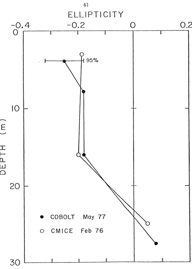
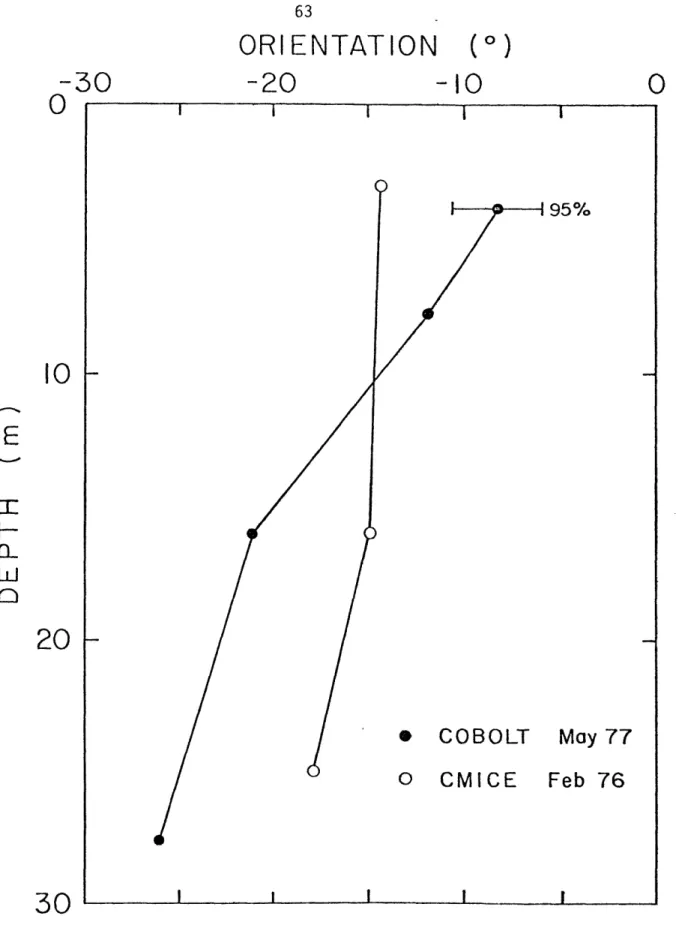
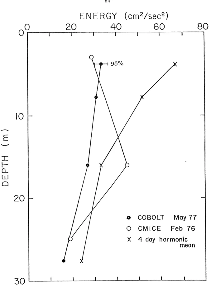
2-6 Semidiurnal tidal ellipses in the CMICE experiment 60 2-7 Vertical profile of semidiurnal ellipticity 61 2-8 Vertical profile of semidiurnal orientation 63 2-9 Vertical profile of semidiurnal kinetic energy 64 2-10 Semidiurnal ellipses for depth-averaged currents 66

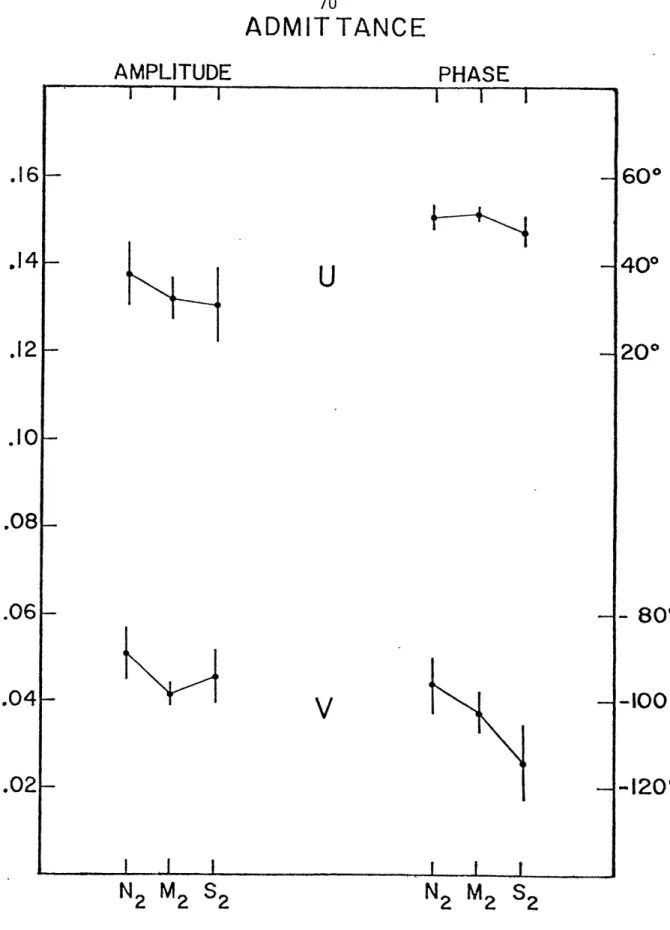
2-11 Band structure of semidiurnal admittances 70

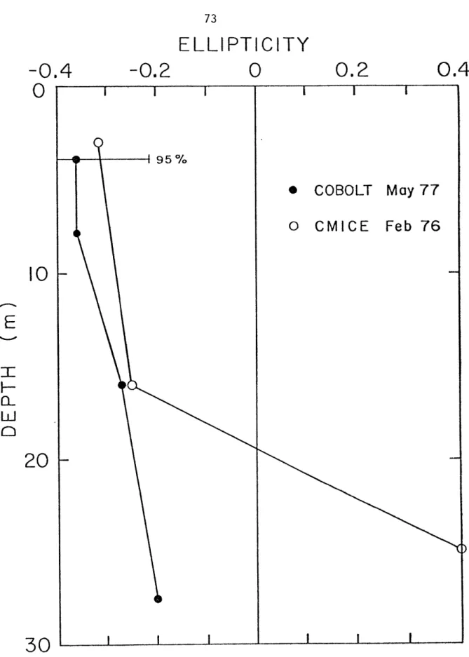
2-12 Vertical profile of diurnal ellipticity 73 2-13 Vertical profile of diurnal orientation 74 2-14 Vertical profile of diurnal kinetic energy 76 2-15 Diurnal ellipses for depth-averaged currents 77

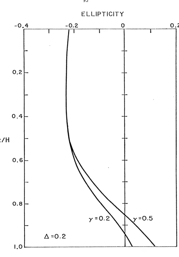
3-1 Theoretical vertical profiles of semidiurnal ellipticity 93

3-2 Theoretical vertical profiles of semidiurnal orientation 94

3-3 Theoretical vertical profiles of diurnal ellipticity 96

3-4 Theoretical vertical profiles of diurnal orientation 97 3-5 Geometry of the step shelf tidal model 102

3-6 Ellipticity versus offshore distance for perfect

reflection (r'=1) and several positive incidence angles 109 3-7 Ellipticity versus offshore distance for perfect

reflection (r'=1) and several negative incidence angles 110 3-8 Orientation angle versus offshore distance for perfect

reflection (r'=1) and several incidence angles 112

3-9 Ellipticity angle versus offshore distance for imperfect

3-10 Ellipticity versus offshore distance for imperfect

reflection (negative incidence angle) 116 3-11 Orientation angle versus offshore distance for imperfect

reflection 117

3-12 Ellipticity versus orientation angle at y=O; incidence

angle varied while holding reflection coefficient constant 120

3-13 Ellipticity versus Orientation angle at y=O; reflection

coefficient varied while holding incidence angle constant 121 3-14 Ellipticity versus Orientation angle at y=O; varying

incident wave frequency 122

3-15 Ellipticity versus Orientation angle at y=O with COBOLT

observations plotted for three semidiurnal frequencies) 124

3-16 Plot of ln(H -H) versus offshore distance at COBOLT

site, plus linear curve fit 130 3-17 Comparison of modelled depth dependence with actual depth

profile off Tiana Beach 131

3-18 Orientation angle versus offshore distance for depth

dependent model 138

3-19 Ellipticity versus offshore distance for depth dependent

model 139

3-20 Kinetic energy versus offshore distance for depth

dependent model 141

3-21 Dissipation versus offshore distance for depth dependent

3-22 Free surface elevation versus offshore distance for depth

dependent model 144

4-1 Twenty-two day average sigma-t cross section at the

COBOLT site 161

4-2 Twenty-two day average Brunt-Vaisala frequency profiles

at buoys 2-4 164

4-3 Salinity time series from instruments 31 and 34 167

4-4 Sigma-t time series at all levels, buoy 3 168

4-5 Sigma-t energy density spectrum from insts.

21-23 & 31-33 170

4-6 Temperature energy density spectrum from

insts. 21-23 & 31-33 171

4-7 Onshore velocity energy density spectrum, insts 32-32 172

4-8 Alongshore velocity energy density spectrum, insts 32-33 173

4-9 Kinetic energy density at 15 m for Sept., 1975 experiment 177

4-10 First three vertical velocity modes at buoy 3 179

4-11 First three horizontal velocity modes at buoy 3 181

4-12 Fitted first baroclinic mode at buoy 2: onshore

velocities 184

4-13 Fitted first baroclinic mode at buoy 2: alongshore

LIST OF TABLES

TABLE _PAGE

1-1 Summary of data returns from Tiana Beach site 31

2-1 The wavelength of the semidiurnal tide 47 2-2 The tidal components used to construct the reference

time series ₅₂

2-3 The semidiurnal admittances and coherences ₅₆ 2-4 The band structure of the semidiurnal admittances 69

2-5 The diurnal admittances and coherences 71

4-1 Numerical values of T, S, N, and sigma-t: buoy 3 ₁₆₁ 4-2 Longshore mean currents at all instruments 165

4-3 Isopycnal displacements for buoys 2 & 3 for all levels:

12 hr., 18 hr., and 24 hr. periods 175

4-4 _{Energy distribution among modes 0-2; buoys 2-4; 12 hr.,}

CHAPTER I

THE COASTAL BOUNDARY LAYER AND THE COBOLT EXPERIMENT

A. Introduction

The coastal regions of the world's oceans have been the subject of increased interest among physical oceanographers in the last decade. This narrow band of shallow water surrounding the continents has long been regarded as too insignificant to affect the great volume of the deep ocean, and as too complicated to conform to simple dynamical theories. The economic and environmental considerations of offshore fisheries and energy related activities, however, have promoted new scientific interest in the dynamics of the continental seas as an important study in its own right. Improved measurement capabilities have also spurred interest and have led to the realization that shallow water dynamics are not as complicated as originally supposed (see reviews by Niiler (1975) and Winant (1978)). A complete understanding of the interaction of these regions with the rest of the ocean may yet prove the shelf's importance to the deep ocean if only as a boundary condition.

The breadth of the continental shelf is by definition limited to

areas within the one hundred meter isobath (Sverdrup, Johnson, and Fleming, 1942), though shelf studies often pass beyond the continental shelf break or continental slope in order to include important

conditions in the transition of shallow to deep ocean flow. Off the east coast of the United States, specifically in a region known as the Middle Atlantic Bight, the shelf extends typically to an offshore distance of 100 km. A representative cross section of this particular region is shown in figure 1.

The eastern continental shelf is often subdivided further into the areas depicted in figure 1: a region of sharp topographic change, known as the shelf break; inner and outer self regions; and, a narrow coastal boundary layer (CBL) close to the shore. The dynamical dissimilarities of the inner and outer shelf, and the shelf break, often noted as the basis of this classification scheme, are summarized in Beardsley, Boicourt, and Hansen (1976).

The region that is of interest here is the coastal boundary layer. This term is applied to a band of water on the order of 10 km wide, which is small compared to the width of the continental shelf, but large compared to the several hundred meter width of the surf zone or littoral zone. From a physical standpoint, the coastal boundary layer is the region where offshore currents adjust to the presence of the coast.

Early work on the Great Lakes (Csanady, 1972) has revealed features which are peculiar to the coastal boundary layer. In particular, observational evidence and theoretical modelling led to

the concept of a coastal "jet" (see Csanady, 1977 for more

details)---the primary mechanism by which the nearshore waters respond to transient meteorological forcing. With regard to the relatively

20

40

60

80

100

150

200

250

Cross section and classification of the Middle Atlantic Bight continental shelf

\ A

!00

uncomplicated dynamics of large lakes, this model has substantially increased the understanding of coastal boundary layer processes.

While application of the coastal jet theory to oceanic coastal boundary layers is straightforward, observational confirmation is more difficult since suitable current observations in the coastal region are rare. And, what observations do exist are more difficult to interpret than the equivalent Great Lakes observations due to the presence of strong tidal currents and large scale flows associated with the rest of the shelf. So, it appears that two additional time scales are important in the oceanic coastal boundary layer: the mean circulation, and tidal frequency motions.

As part of the Coastal Boundary Layer Experiment (COBOLT), this thesis is directed toward developing an understanding of the tidal frequency motions of the coastal boundary layer. This goal is pursued

by presenting a description of the tidal currents of the coastal zone

followed by a conceptual model that reproduces many of the observed features of the barotropic or surface tide. The question of internal or baroclinic tides is addressed with a detailed description and comparison to existing models.

B. The COBOLT experiment

The COastal BOundary Layer Transect (COBOLT) experiment was designed specifically to study the complexity of the coastal zone. Drawing from experience gained on the Great Lakes and taking advantage of newly developed instrumentation, it was planned to provide a

16

detailed spatial and temporal picture of the wind-driven coastal boundary layer, the currents induced by tides, and the interaction with the large scale circulation of the continental shelf. The motivation for the experiment was provided by proposals to locate power stations offshore, together with the realization that very little was known observationally about the coastal boundary layer. The project represents the joint efforts of the Woods Hole Ocean-ographic Institution and Brookhaven National Laboratory (BNL).

C. The experiment site

The southern coast of Long Island was chosen for the site of the COBOLT experiment because of its similarity to an idealized straight coastline. This region is shown in figure 2. Tiana Beach, the shore location point, is 135 km east of New York City and the New York Bight Apex, and 60 km west of Montauk Point, the terminus of Long Island. The approximate coordinates of the experiment are 400 45'N and 720 30'W. The site enjoys easy access from the protected waters of Shinnecock Bay through Shinnecock Inlet which is about 6 km east of Tiana Beach, and is also within reasonable distance of Brookhaven National Laboratory.

Geographically, the coast of Long Island forms part of the northern boundary of the Middle Atlantic Bight. The coast itself is a virtually continuous barrier sand bar, with only four or five breaks for entrances to protected bays in its 195 km extent. The shallow water topography is formed from loose, large-grained sands and is

5 0

uN

0

AN

TIANA

BEACH

ATLANTIC

OCEAN

Figure 1-2 The south shore of Long Island

0

N G

410

18

remarkably smooth with minor "swale" features (Swift et al., 1973) as the only irregularities.

While topographic features are smooth and lead to relatively uncomplicated dynamics, there are other features of the COBOLT experiment site which may complicate the interpretation of the data. The presence of Long Island Sound, for example, is likely to have some

effects on COBOLT measurements. Tidal observations (Redfield, 1958 and Swanson, 1976) show strong aberrations in tidal propagation characteristics up to 50 km away from the entrance to the Sound. A

close-to-resonant response gives rise to very large currents in the vicinity of Montauk Point and tidal phases that change rapidly from point to point. Also, the Sound is a major source of fresh water (Ketchum and Corwin, 1964). Since the runoff from Long Island itself is relatively minor, the Sound is probably the origin of any fresh-ening that occurs at the COBOLT site.

In addition, the proximity of Shinnecock Inlet may influence the measurements. Though it is narrow (about 200 m wide) and less than 5 m deep at most points, visual surveys indicate that the plume of tidal discharge reaches 2-3 km out to sea and is visible as far down-shore as 6 km. Thus, it is conceivable that moorings which are close to

shore may show the effects of being near to the inlet.

D. Coastal measurements

One of the major hurdles encountered in mounting a near-shore measurement program is that of choosing adequate instrumentation. It

19

is well known that current meters mounted near the surface are profoundly affected by high frequency gravity waves even when carefully conceived sampling and averaging schemes are employed. Instruments which sample speed and direction (via Savonius rotor and vane), such as the VACM or Aanderaa current meters, are particularly susceptible to rectification of wave-induced orbital velocities, even when mean velocities are of comparable magnitude (McCullough, 1977).

Taut rope moorings also contribute to measurement errors in several ways. _{Strong currents, such as those encountered in the coastal zone,} cause sizable vertical excursions of the instrumentation. Also, surface layer fluctuations can be transmitted down the flexible rope to contaminate measurements at deeper instruments. Finally, the lack of torsional rigidity may introduce directional errors.

The presence of a nearby coast adds measurement problems of its

own. _{In addition to the increased possibility of human interference,}

the nearness of the coast causes low frequency currents to be polarized in _{the alongshore direction and increases the probability of} measuring important- onshore velocities incorrectly. For example, in a strong alongshore current of 50 cm/sec, as little as one degree of error in orientation can cause a 1 cm/sec error in the onshore velocity--an amount which is comparable to the true mean value of the

onshore currents.

To the list of difficulties to be overcome in instrument and mooring design must be added the demand that both temperature and salinity be measured. _{Unlike the deep ocean, where tight}

temperature-20

salinity properties make a functional relationship between the two possible and eliminate (somewhat) the need for salinity time series, shallow coastal waters have -no such links. Density variations are controlled by salinity at certain times of the year and by temperature at other times, and both signals are usually large. In order to separate dynamic effects, time series of both parameters are essential. Despite the difficulties, several useful experiments have been carried out in the coastal zone of the Middle Atlantic Bight using conventional measurement techniques. Two of the most notable of these are the EG&G Little Egg Inlet experiment (EG&G, 1975) and the New York Bight MESA project (Charnell and Hansen, 1974). Even in view of these successes, a concerted effort was made in the COBOLT experiment to eliminate the potential sources of error in conventional instrument-ation and moorings, _{and to add measurement capabilities not available} in earlier studies. These requirements necessitated a radical departure from common deep water mooring design and instrumentation.

E. The COBOLT instrumentation

The mooring platform for the COBOLT instruments, the "Shelton Spar", was developed for coastal work off La Jolla, California. It is constructed of sections of 2 1/2" diameter PVC pipe (Lowe, Inman, and Brush, 1972). The moorings utilize specially designed universal joints to allow the spar to articulate freely at the several junction points, without sacrificing too much of -the inherent rigidity of the pipe. Since it is torsionally rigid (torsional variations are

estimated by the manufacturer to be less than 10), the mooring requires only one compass to determine the orientation of the four current meters mounted on it in rigid steel cages. With the large buoyancy element employed, the mooring also tilts very little; typically 100 in a 50 cm/sec current. Thus much of the vertical and rotational movement of conventional moorings is eliminated.

Instrument packages consist of two temperature probes--one "local" and one "remote"--and induction-type conductivity sensor, and a Marsh-McBirney, Inc. Model 711 electromagnetic current meter. The current meters have two orthogonal sets of electrodes mounted on a 2 cm diameter vertically oriented cylinder. The principles of operation of the electromagnetic current meter are discussed in Cushing (1976).

A typical mooring configuration, pictured in figure 3, employs four of the instrument packages described above, plus one compass, two orthogonal tilt sensors, an in situ data processor, and a radio transmitter. _{Sensor outputs are low-pass filtered in real time with a} five second time constant (the stated response time for the sensors is typically one second) and continuously integrated in the data processor. _{Averaged values of the measured parameters are then} transmitted, on command, to a shore station at Tiana Beach. Operators can therefore adjust the sampling rate or detect faulty instruments while the experiment is in progress. _{Experiment duration is limited,}

typically to one month periods, by the large power consumption of the transmitter. _{Further technical details are available in Dimmler, et.} al. (1976).

Radio Telemetry

link to

BLN

3.87.8

m-16.0 m

28.4m~

.--

Floatation collar

ECM

ECM

Data processor

ECM

Compass and inclinometer

Shelton spar

ECM

Battery

container

---.-

-

30.8m

Fu *- Configrat 6 io o a t C spar buoy

In spite of the care taken in its design, the COBOLT moorings have not been perfected yet. An experiment somewhat related to COBOLT, the Current Meter Inter-Comparison- Experiment (CMICE), was conceived as an opportunity to test the merits of the spar system against coventional moorings and instruments. _{In this experiment, described in detail by} Beardsley, et. al. (1978), six moorings were deployed off Tiana Beach in a line parallel to the shoreline and 6 km from the beach. Four of the moorings were conventional taut rope moorings instrumented with a variety of current meters (mostly of the Savonius rotor and vane type), while the remaining two moorings were the Shelton spars. A comparison of the measurements of these instruments suggest that there are some deficiencies in the COBOLT moorings and intrumentation. The sources of possible error in the COBOLT velocity measurements are:

1. _{Errors due to mis-orientation of the single compass or}

misalignment of current meters with respect to the compass.

2. _{Errors due to a shift in the zero point of either or both of} the current meter axes.

3. Errors due to asymmetric gain adjustment of the two current

axes or non-cosine response of the sensors.

F. COBOLT experiments and data

After some pilot studies, the full COBOLT array of four spar buoys was first deployed in May, 1977. The location of each of the four buoys and their relationship to surrounding features is shown in

24

figure 4. The buoys were placed approximately 3 km, 6 km, 9 km and 12 km away from the shore, and stand in 20 m, 28 m, 30 m, and 32 m of water respectively.

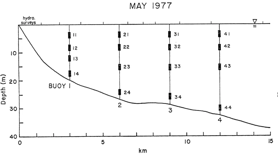
The instrument configuration, bottom profile, and location of daily hydrographic casts (described subsequently) is shown schemat-ically in figure 5. Instruments are identified by a sequence of two numbers: the first corresponding to the number of the buoy on which the instrument is mounted, and the second corresponding to the order, starting at the top, in which it is mounted. An attempt was made to place instruments at standard depths: the shallowest at 3.8 meters below the surface; intermediate instruments at 7.4 meters and 16.0 meters; and the deepest at 2.4 meters above the bottom. Buoy 1 is the exception to this rule with one instrument at 12.3 meters instead of

16.0 meters.

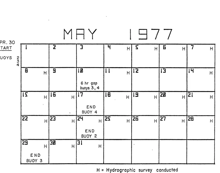
The spars were launched on April 29, 1977, and regular data recovery from all four buoys was initiated on April 30. Because of non-uniform power drain, endurance of the different moorings varied significantly. Buoys 1 and 3 were operational until May 29; buoy 2 until May 24; and buoy 4 until May 17. The operation period of the experiment is summarized in figure 6.

The quality of instrument records (containing temperature(l), temperature(2), salinity, X velocity and Y velocity).is good, with the exclusion of buoy 1 which suffered numerous irrecoverable data gaps. These gaps were uniformly spread throughout the data and amounted to a total of 140 hours out of a total duration of about 700 hours or

I I I 1

0

2

3km

3.

4,

30'

Locations of the four spar buoys of the May, 1977 experiment

MAY 1977

hydro.

5

10

km

Figure 1-5

Depth profile off Tiana beach, location of spar buoys, instrument packages,

and hydrographic survey stations

20

.c

S

4-30

40

APR. 30

START

BUOYS

2

3

4

MRY

H77

12

3

HH

7

H

a

H

_H

_H

6 hr gap

H

H

16

H

H

H

H

END

BUOY 4

22H

_H

_4H

_S

_H

_H

_H

H

END

25

_H

_H

H

E

ND

H Hydrographic survey conducted

Figure 1-6 Calendar for the May, 1977 experiment showing buoy duration

one-fifth of the total time. One stretch of ten days was relatively Eree of long gaps and consequently can be used for limited compar-isons, but the rest of the record was abandoned as unacceptable for tidal analysis. Data from the other three moorings, buoys 2-4, showed only occasional, short data gaps during periods of high speed flow. These gaps never exceeded 6 hours in length.

In conjunction with the continuous buoy measurements, daily hydrographic surveys of the area were conducted. These STD measure-ments were made from a small vessel at ten semipermanent locations along a line coincident with the spar transect. The spacing of the stations, about 1 km, was chosen to give more detailed resolution of the coastal boundary layer than was provided by the 3 km spacing of the spar buoys. Although they were performed only in fair weather, and although they are aliased by tidal fluctuations, the hydrographic surveys are a valuable source of information in interpreting the spar data.

In view of the questions that have arisen concerning the data quality of the spar system, and in an effort to assure the generality of the tidal analysis to follow, results from two other moorings will be included in the discussion: a "reference" mooring from the CMICE

experiment, and the COBOLT pilot mooring.

The mooring chosen from the CMICE experiment was deployed by the

MESA New York Bight project and has been used extensively in their field program. The instrumentation consisted of four Aanderaa RCM-4 current meters; three mounted on a subsurface taut wire mooring, and a

fourth mounted beneath a surface spar buoy to reduce wave-induced biases. The mooring is shown schematically in figure 7. One instrument at 11 meters below the surface did not function. The experiment was conducted at the COBOLT site in February, 1976 with this particular mooring positioned 6 km offshore at approximately the same location as buoy 2 of the May COBOLT experiment. The mooring was designated as #5 in the CMICE experiment and since this conforms to the convention used here, it is retained in Table I and in further references.

The COBOLT pilot mooring, launched in September, 1975, was a single mooring placed 11 km offshore at roughly the same location as buoy 4 of the May, 1977 experiment. It had working instrument packages at 7.8 m, 16.0 m, and 27.0 m and was in 32 m of water. The details concerning this mooring and the others employed in this

analysis are summarized in Table 1.

Although it seems a bit capricious to compare current observations taken during different seasons and separated in time by more than a year, there are elements of the signal which are expected to remain the same throughout the year. Even if meteorological forcing and stratification are different, the tidal signal should be determin-istically related to well-known forces at all times. Including these additional moorings will allow comparison between certain aspects of the COBOLT experiment spar buoys and the relatively well-understood Aanderaa current meters of the CMICE experiment, and will also assure that measurements are somewhat representative of different seasons and conditions.

Spar buoy

Auxiliary

float

9.0

M-10.0 m-(

1 1.0

m-15.7

m~n

25.0

in-Dan forth

anchor

3.0m

I 1#

buoyancy

955t#:

buoyancy

Aanderoo

3/16" Wire

Aanderoa

Aande raa

A

coustic

52

rope

53

54

release

Clump anchor

Figure 1-7 Configuration of MESA-CMICE mooring #5

TABLE 1-1

SUMMARY OF DATA

RETURNS FROM THE TIANA BEACH SITE

Water Dist. Depth of working Date of Exp.

Sept., 1975

Feb., 1976

May, 1977

No. Duration Depth offshore Current meters

0 640 hr 32.6 m 11 km 4.2 m, 16.5 m, 29.7 m 5 697 1 240 2 577 3 700 4 385 26.5 20.3 27.7 30.8 32.3 6 3.0, 15.7, 25.0 3 3.8, 7.8, 12.3, 17.9 6 3.8, 7.8, 16.0, 25.3 9 3.8, 7.8, 16.0, 28.4 12 3.8, 7.8, 16.0, 29.9

G. Data Processing

The data sampling scheme is unique to the spar system and presents minor problems of its own. Buoys were interrogated at separate times and at intervals that ranged from five minutes to several hours. Since ordinary time series analysis demands that sampling intervals be uniform and that measurements for comparison be taken at a common time, the COBOLT data were adjusted to a common time base with a one-hour sampling interval (one hour was by far the most common interval in the data). This was achieved by first averaging all data over a one-hour time period and then interpolating values to the closest whole hour. The interpolation scheme was a third order polynomial that used four data points (two on either side of a gap) to determine the value of the function on the hour. This method has the advantage of eliminating the sharp bends introduced by linear

interpolation, and of filling gaps in strong tidal flows with consistent curves. For periodic functions, for example, the poly-nomial interpolation gives a good visual fit for record gaps of up to one-half of a period. Using this as a guideline, COBOLT data gaps were filled only if they were less than or equal to 6 hrs in duration;

that is, half a semi-diurnal tidal period.

The X and Y component velocities output from the current meters were converted to east and north components using the headings from the single on-board compass. Then the coordinate system was rotated

by 220 to conform to the local coastline at Tiana Beach. The uncertainties usually associated with this maneuver are quite small

here due to the uniformity of the coastline and topographic features. The result is a coordinate system with the X axis aligned alongshore

to the east-northeast and the Y axis pointing onshore to the north-northwest.

The salinity time series from the May, 1977 experiment required special attention. Mean salinities (computed from the measured conductivities) differed by as much as 3 o/oo from adjacent instru-ments and by as much as 2 o/oo from values obtained from nearby STD measurements. These aberrant salinity measurements resulted in large,

persisent inversions in the computed density. Since there was nothing to suggest that these aberrations were other than the result of a constant calibration offset, an effort was made to correct them using two different procedures. In the first, salinities were offset enough to eliminate all density inversions, while in the second, salinities were made to conform to nearby daily hydrographic survey salinities in

a least-squares sense. These adjustments agree quite closely and give credence to the notion that errors were due only to calibration offsets and not to instrument drift or malfunction.

CHAPTER II

NEARSHORE TIDAL CURRENT OBSERVATIONS

A. Introduction

An examination of the current records from any coastal experiment in the Middle Atlantic Bight shows that they are dominated (vis.ually at least) by tidal oscillations. Even though such short period oscillations do not transport mass, momentum, or other passive properties of the water column (except in non-linear cases), the large amplitude of the tidal signal often obscures other aspects of the records--particularly if the observation period is short. As a consequence, an understanding of some of the slower and less obvious processes of the coastal region may be improved by an understanding of the tides.

Certain aspects of coastal dynamics may also be directly controlled or influenced by the surface tides. Internal waves, for example, are known to be generated by tidal currents interacting with the topographic features found in coastal areas (Rattray, 1960). There is also evidence (Bowden and Fairbairn, 1956) that the tidal currents control the high background level of turbulence observed in coastal regions--acting, in effect, like a stirring rod. This is closely related to the question of tidal dissipation, much of which is presumed to occur on the continental shelves of the world's oceans (Munk, 1968). Little is known about the mechanisms by which this is

accomplished or the regions in which it occurs. A study of coastal

tides may serve to illuminate the subject.

Because of the deterministic nature and relatively high frequency of tidal currents, information can be extracted from relatively short duration experiments. The thirty days of data gathered during May

1977 is suitable for some forms of tidal analysis and will be used in

the hope of elucidating some of the local dynamics of the nearshore region, comparing the performance of the COBOLT mooring system to other systems, and as a first step in obtaining detided records for analysis of low frequency phenomena.

B. Tidal Analysis

Tidal analysis is traditionally carried out using the harmonic method introduced by Lord Kelvin in 1867. The frequencies, ., at which forcing occurs, are obtained from expansions of the tidal potential (Doodson and Warburg, 1941) and used in the expression

F(t) = a. cos (W.t + #.) _{1 1 1} , (1)

which is then fitted to the data in a least-squares sense by

adjusting the constants a. and *. This method requires long records, typically greater than a year, in order to resolve some of the closely spaced constituents, and to provide statistical stability since weak tidal "lines" are often obscured by background noise. Also, the similarities in responses to given forcing are concealed in

the multitude of different amplitudes and phases. So it is not well suited to the analysis of short records.

In harmonic analysis, statistical stability is usually maintained at the expense of resolution. That is, averaging the spectra of many different pieces or realizations, or averaging across frequency bands in individual spectra reduces the ability to resolve different frequencies but improves the reliability of the spectral estimates (Bendat and Piersol, 1971). _{In analyzing short time series this} problem is critical since the averaging procedure obscures spectral differences between adjacent frequencies. In tidal analysis, for example, fifteen days is _{the minimum record length that allows} resolution of the principal lunar and principal solar constituents since these components differ by one cycle in fifteen days. Averaging spectral estimates over n frequency bands limits the resolving capabilities to signals which differ by n cycles in fifteen days. Thus, reliable estimation of the tidal constituents by

spectral or harmonic- techniques depends on the availability of fairly long term observations. If this criterion is not met the so-called

"admittance approach" offers a viable alternative.

The method used to analyze the COBOLT data, the admittance approach, is described by Munk and Cartwright (1966). Basically, if one hypothesizes a linear, causal relationship between two time series, x(t), which is termed the "input", and y(t), which is termed the "output", the most general linear relationship between the two can be defined by the convolution integral,

y(t) = f x(t') h(t-t') dt' ₍₂₎

where h(t) is known as the impulse response function. Defining the Fourier transform by capital letters, i.e.,

F() = f f(t) e dt , (3)

and taking the transform of equation (2) gives

Y() = H() X(W) , (4)

where H(o) is the transfer function or admittance.

Since one rarely works with direct transforms, but rather with spectra, the following definitions are useful:

AUTO-SPECTRUM CROSS-SPECTRUM (where * indicates a (4), it follows that S (W) = X(o) X*(o) S (o) = X*(W) Y(W) ; xy (5)

complex conjugate) from which, using equation

38

If x(t) is a periodic function, say

x(t) = a exp iwt , (7)

equation (2) assumes a particularly simple form

y(t) = H(W) x(t) . (8)

This form is especially useful in generating the output function, since it is more easily computed than equation (2). It also reveals the conceptual basis of the admittance; it is a measure of the spectral linkage between the input and the output functions.

The primary advantage of the admittance analysis is the ability to reduce noise to well-defined levels without sacrificing resolu-tion. This is accomplished by invoking the so-called "Credo of Smoothness" (Munk and Cartwright, 1966) which states that admittance

amplitudes and phases are relatively smooth over broad frequency bands. This is based on the observation that the response of most physical systems does not change too abruptly if the frequency of the forcing or input is altered. Exceptions to this argument are systems that are being forced at close-to-resonant frequencies. The successful use of the admittance approach does not depend on a high degree of resolution because the admittance function varies so slowly with frequency that any structure in it can be discerned with short records or low resolution analysis. Because the input is generally a

39

well-known function for which long time series are available, high resolution analysis of output time series can be obtained from equation (8) _{once the form of the admittance function is known.}

Instead of resolution and stability, the questions to be answered in _{the admittance approach center on the proper choice of an input} function. _{The ideal input function is related so closely to the} output that the admittances necessarily conform to the "Credo of Smoothness"; it is available (or can be constructed) for long enough time periods to allow the desired resolution; and, it is free of noise.

The analysis offers another important advantage. Because admittances are formed from ratios, they tend to divide out some of the numerical effects of the finite Fourier transform. This is again of interest in the processing of short time series where information from narrow frequency bands is spread out into relatively broad bands

by the effective filtering of the transform process. Because the transform alters both the input and output functions in a similar manner, these effects are minimized with the use of the admittance.

Finally, the analysis provides a measure of how much of the output is coherent or phase-locked to the input. This measure is the squared coherence, defined as (Bendat and Piersol, 1971)

2 2

S

(m)

S

W(S

)

(9)

That part of the signal which has random variations in amplitude and phase, such as weather fluctuations or intermittent baroclinic

40

effects, is summarily classified as noise. Ensemble averages of the admittances have, as a result, well-defined errors expressed in terms of the coherence. A particularly simple form for the variance of the

real and imaginary parts of the admittance (which are distributed normally) is given by Munk and Cartwright as

2

JH(W) ~

1

-

y(

V 2N 2

where N is the number of statistical degrees of freedom and Y is the true coherence.

Traditionally the equilibrium tide is chosen as the input function when analyzing short duration tide gauge or current meter data (see Filloux, 1971 and, Regal and Wunsch, 1973). The equilibrium tide, however, is computed from the tidal potential under the assumption that the earth is entirely covered by an infinitely deep ocean. It consequently does not account for variations that occur as the result of the presence of land masses and topography. In shallow, coastal waters it is well-known (Defant, 1961) that direct forcing by astronomical bodies plays only a minor role. The main forcing comes instead through interaction with the deep ocean tides at the continental shelf outer boundaries. Here the pceanic tidal currents are constricted by the rapid decrease in water depth and act through continuity to drive more energetic flows on the continental shelf than could be achieved through the action of direct astronom-ical forcing alone. (Further discussion of this subject is contained in the following chapter.) For this reason a series of coastal tide

height observations is presumably a much more appropriate input function for analysis of coastal tidal fields. So, following a procedure suggested by Cartwright, Munk, and Zetler (1969), a reference series computed from the tidal harmonics of a nearby tide station is used as the input function in analyzing the COBOLT data.

C. The tidal ellipse

The presentation of the data is conveniently accomplished through the use of the tidal ellipse. Given the orthogonal velocities u and

v, which are periodic with some frequency w, the complex vector u +

iv can be formed. This vector may be decomposed into two constant, complex vectors A+ and A~, rotating in opposite directions: clockwise (-) and counterclockwise (+). Algebraically this is expressed as

+ iWt - -iWt

u + i v = A e + A e (11)

These rotating vectors alternately add to, or subtract from one another producing the characteristic shape of the tidal ellipse. The phases of the vectors determine which direction the ellipse is oriented.

The parameters which succinctly describe the ellipse are the ellipticity and the orientation. They are illustrated in figure I and defined (respectively) by:

-

L i-

A=

A

12)

A-ELLIPTICITY

E= m/M

ORIENTATION

TIDAL

ELLIPSE

Definition sketch of the tidal ellipse

argA + _{arg A (13)}

2

In geometric terms, the ellipticity is the ratio of the minor axis of the ellipse to its major axis. It is: positive if the complex current vector u + iv rotates in a positive sense (counterclockwise); negative if the vector rotates in a negative sense (clockwise); equal to one if the vector traces a perfect circle; and equal to zero if the ellipse degenerates into a line.

The orientation measures the angle between the major axis of the ellipse and the positive x axis. (The x axis will point alongshore and the y axis onshore throughout this work.) It is constrained, by definition, to fall between ±900.

These quantities are introduced, not only to make the results easier to visualize, but as diagnostic tools for determining the dynamics of the tides. While the free surface co-phase (lines of constant phase) and co-amplitude (lines of constant amplitude) contours are valuable in this respect, the velocity field is quite sensitive to other dynamic (e.g., frictional) effects. This sensitivity is a consequence of the rotation of the earth which introduces ellipse characteristics that are peculiar to certain dynamics. Thus, it is advantageous to employ information from both surface and velocity fields in attempting any interpretations.

D. Tidal observations in the Middle Atlantic Bight

Under a common classification scheme which uses a ratio formed from the _{amplitudes of four prominent semidiurnal and diurnal} constituents, the tides of the Middle Atlantic Bight are characterized as predominantly semidiurnal. This ratio (Defant,

1961),

Ky +0O_{1 1 (14)}

M + S ' 2 2

ranges from 0.19 at Sandy Hook, New Jersey to 0.33 at Montauk Point, New York, and averages about 0.25 for the Middle Atlantic Bight in general.

The M2 constituent is the largest; the ratio M2 :S2 typically being about 5:1 (Shureman, 1958).

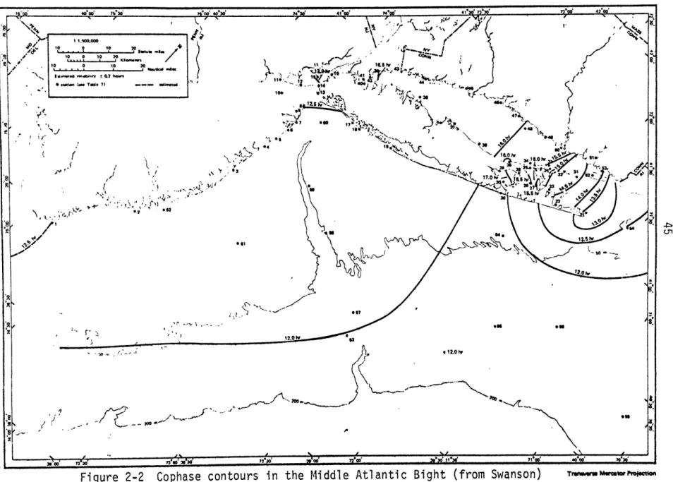
The Atlantic Ocean semidiurnal tide arrives everywhere at the edge of the continental shelf at roughly the same instant (Dietrich, 1944) _{and progresses with cophase contours paralleling the New} Jersey-Delaware shore. _{To the north, the presence of Long Island} Sound affects propagation characteristics markedly with its near-to-resonant response (Swanson, 1976). _{Cophase lines (see figure 2,} taken from Swanson's work) bunch up around Montauk Point and distort normal tidal patterns many kilometers away from the Sound itself. As a consequence, the tide propagates to the east (towards the entrance to the Sound) along eastern Long Island and the west along central and western Long Island (in conformity to the rest of the shelf). The contours also show that the propagation pattern divides somewhere near the COBOLT region (station 20 on Swanson's map). Thus this area marks the transition between the tidal regime of the Bight and that

TraWW-- M --tloction

of the Sound, and complicated interactions between the regions may be expected.

A crude estimate of the semidiurnal tidal wavelength, which will

be valuable in the ensuing discussion, may be made by using the phase lags from the NOAA Tide Tables with the kinematic relationship between wave speed and wavelength,

Wavelength = Phase Speed x Period. (15)

These figures suggest that this wavelength is about 1500 km (Table 1). The diurnal tides are not so well documented as the semidiurnal but seem to progress from north to south with cophase contours perpendicular to the isobaths and coastline rather than parallel to them (Dietrich, 1944). _{In view of the lack of published information,} it is difficult to characterize them except in noting that their propagation patterns differ noticeably from those of the semidiurnal constituents.

Tidal current measurements on the shelf, accompanied by the appropriate analysis, are generally sparse. Haight (1942) compiled current measurements from about fifty light ships on the East Coast in one of the earliest studies of tidal currents. Most of these lightships were located at the entrance to large harbors or on dangerous shoals and consequently are very complicated examples of nearshore tidal currents. _{Some general observations may be made,} however. First of all, tidal ellipses are usually very elongated

TABLE 2-1

SEMIDIURNAL WAVELENGTH COMPUTATION

Guage Distance Location from Sandy Hook Shinnecock Inlet 138 km Fire Island Jones Inlet 39

High & Low Phase Water Interval Speed

0.83 hr 1.13 hr 144 km/hr 0.63 0.32 0.48 0.45 114 Wave-length 1791 km 1413 104 1295

(the ellipticity is much less than one) at nearshore locations and more circular at offshore points. And, velocity vectors rotate almost exclusively in the clockwise direction; at 94% of Haight's observation points, according to Emery and Uchupi, 1972.

Form measurements on the outer shelf, Flagg (1977)found that up to 50% of the total variance at individual current meters was due to the combined effects of diurnal and semidiurnal tides. Traschen

(1976), using the same data set, notes that semidiurnal tidal ellipses _{are virtually circular and oriented in the cross-isobath} direction, while diurnal ellipses are very elliptical and are oriented along isobaths.

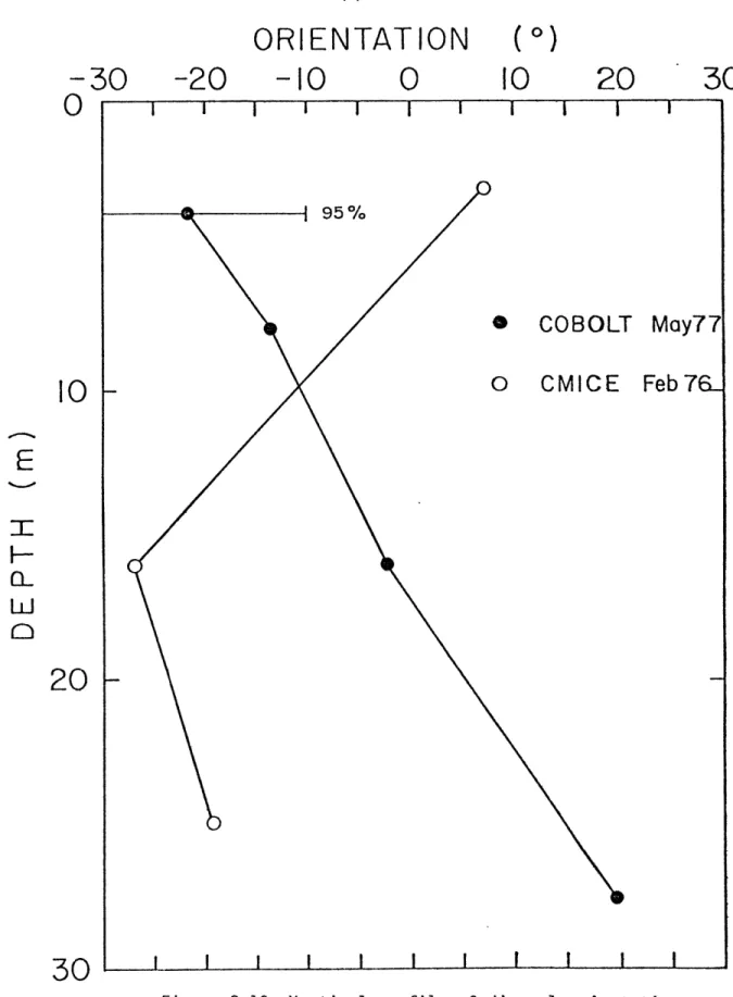
Nearshore current measurements, _{such as those of Patchen, Long,} and Parker (1976) in the New York Bight Apex, show the pronounced effects of a nearby shoreline, particularly if the measurements are not influenced by the presence of harbors or bays along that shore. If there is a solid boundary, onshore tidal velocities must be

diminished to satisfy the boundary _{condition at the shore.} This condition causes the tidal ellipses to elongate into very eccentric (low ellipticity) forms. Figure 3, taken from Patchen, Long, and Parker, shows the semidiurnal tidal ellipses from their experiment. In addition to the elongation of the tidal ellipses, it is noted that the major axes show a noticeable deviation from a shore-parallel orientation. Typically this orientation "tilt" angle is small--anywhere from 5

0-10

8 meters above bottom

3 meters or less above bottom

74*0D'

I uperO Say New York

Rockaway Pont Sandy Hook S6 0 50 cm/sec New Jersey I 520.000 0 5 10 K 5 N0 m0 74*00' 73*M'

Rotation is predominantly clockwise at 8 m (26 _{the bottom, counterclockwise at 3 m (10 Ift) or} ft) above Arrows indicate direction of progress of the maximum M2

flood current velocity.

less above the bottom. _{Current velocity vectors rotate 3600 in 12 to 42 hours.} The centers of ellipses are the station locations.

Source: From Patchen et &1 1976

Figure

2-3

Other generalizations regarding the vertical structure of the tidal ellipses can be made from this experiment. It appears that ellipses near the bottom (3 m away) usually exhibit different ellipticities than those near the surface (here they are more circular in shape) and rotate, generally, in the counterclockwise direction. By contrast, tidal ellipses further away from the bottom

(8 _{m) are almost always more eccentric and rotate in the clockwise}

direction.

Measurements near Little Egg Inlet, N. J. (EG&G, 1975), another coastal series available for comparison, are highly influenced by the presence of the inlet. This, as was the case with Haight's analysis, makes generalizations difficult. _{The experiment does show, however,} predominantly clockwise rotation of tidal ellipses (with one exception) and emphasizes the point that large amounts of variance are due to the tides; 33% for year-long records in this case.

There appear to be few other relevant studies of nearshore coastal tidal currents in the Middle Atlantic Bight despite the increased interest in this region. Measurements which do exist usually focus on the lower frequency signal and neglect altogether mention of tidal phenomena. Work on other shelves (e.g. Petrie,

1975), while serving as a useful comparison, will not be pertinent to

the Middle Atlantic Bight because of different deep ocean tidal forcing and topographic features.

E. Analysis of the COBOLT tidal signal

The first step in the analysis of the COBOLT data involved the choice of a reference tide station from which to generate the input time series for the admittance procedure. The station chosen was the tide gauge at Sandy Hook, New Jersey, approximately 140 km to the west of the COBOLT site. This is a reasonable choice if the COBOLT moorings are assumed to be in the tidal regime of the open shelf and not to be too closely related to that of Long Island Sound. It is also the closest one to have operated over the long period of time necessary to obtain stable values of tidal amplitudes and phases for the prediction. It has, in fact, been operational for more than a hundred years.

The tidal constants used to construct the reference time series were taken from Shureman (1958) and represent the results of harmonic analysis of ten years of data. The components employed are listed in table 2 along with appropriate periods, amplitudes, and epochs (the phase relative to the transit of the mean moon over the Greenwich meridian). Non-astronomical tides, such as those due to non-linear and radiational effects, and components with amplitudes that are less

than 2% of the M2 amplitude were ignored.

The input function generated was then subjected to the same procedures as were followed with the current meter data; i.e., overlapping data pieces 360 hours (15 days) long were used with a Fast Fourier Transform routine to give spectral estimates separated

TABLE 2-2

TIDAL COMPONENTS OF REFERENCE TIME SERIES

COMPONENT PERIOD AMPLITUDE

11.96723 12.00000 12.19162 12.42060 12.65835 2.9 cm 13.0 3.4 70.0 15.9 23.93447 24.06589 25.81934 9.0 3.2 4.3 PHASE 243 deg 246 203 218 201 102 105 98