Amplitude and phase variations of surface waves in a laterally heterogeneous earth : ray- and beam-theoretical approach

AMPLITUDE AND PHASE VARIATIONS OF SURFACE WAVES IN A LATERALLY HETEROGENEOUS EARTH:

RAY- AND BEAM-THEORETICAL APPROACH by KIYOSHI YOMOGIDA B.S., University of Tokyo (1980) M.S., University of Tokyo (1982)

Submitted to the Department of Earth, Atmospheric, and Planetary Sciences

in Partial Fulfillment of the Requirements of the Degree of

DOCTOR OF PHILOSOPHY at the

OMASSACHUSETTS INSTITUTE OF TECHNOLOGY October, 1985

Signature of Author:___ _

Department 0rEarth, Atm< pheric,' and Planetary Sciences

Certified by Accepted by: Sean C. Solomon ) Thesis Co-Supervisor Keiiti Aki Thesis Co-Supervisor William P Rrar Chairman, Department of Earth, Atmospheric

WtTIJ

and Planetary Sciences

ARR096

Undgren

AMPLITUDE AND PHASE VARIATIONS OF SURFACE WAVES IN A LATERALLY HETEROGENEOUS EARTH:

RAY- AND BEAM-THEORETICAL APPROACH by

KIYOSHI YOMOGIDA

Submitted to the Department of Earth, Atmospheric, and Planetary Sciences

on October 25, 1985 in Partial Fulfillment of the Requirements for the Degree of Doctor of Philosophy

ABSTRACT

Lateral heterogeneity of the Earth has begun to be mapped extensively by measurements of phase velocities of surface waves since the installation of global digital network. The methods used in such studies are, however, based on simple ray theory: observed phase delays are assumed to be integrations of slowness along the great circles connecting sources and receivers. On the other hand, wave theories for seismic body wave

propagation in a laterally heterogeneous medium have advanced remarkably. Most of these theories are based on asymptotic ray theory. This study tries

to combine these two different developing fields: to improve the resolving power of surface waves to the lateral heterogeneity of the Earth through an inverse method based more closely on full wave theory (asymptotic ray

theory). We chose the Gaussian beam method and applied it to the surface wave problem. This study consists of three principal parts: (1)

derivations of formulations, (2) forward modelling, and (3) inversions of phase and amplitude data for phase velocity, including a non-linear

iterative method.

First, asymptotic ray theory is applied to surface waves in a medium where the lateral variations of structure are very smooth. In such a medium the formulation for points exactly on the ray has previously been given by others. Using ray-centered coordinates, we obtain parabolic equations for

lateral variations while vertical structural variations at a given point are specified by eigenfunctions of normal mode theory as for the laterally

homogeneous case. Following the paraxial ray approximations developed for acoustic or elastic body waves, the formulation at points not only on the

ray but also in the neighborhood of the ray is successfully derived. Final results on wavefields close to a ray can be expressed by formulations

similar to those for elastic body waves in two-dimensional laterally heterogeneous media. The transport equation is written in terms of

geometrical-ray spreading, group velocity and an energy integral. For the horizontal components there are both principal and additional components to describe the curvature of rays along the surface, as in the case of elastic body waves. With complex parameters the solutions for the dynamic ray

iii bell-shaped along the direction perpendicular to the ray and the solution is

regular everywhere, even at caustics. Because of the similarity of the present formulations to the original ones, most of the characteristics of Gaussian beams for two dimensional elastic body waves are also applicable to the surface wave case. At each frequency the solution may be regarded as a set of eigenfunctions propagating over a two-dimensional surface according to the phase velocity mapping.

Special attention to the following points is necessary for surface wave synthesis: (1) the speed of the wavepacket along the ray is the local

group velocity even though the ray path itself is determined by the phase velocity distribution in an isotropic or transversely isotropic medium; (2) surface waves travelling on a spherical Earth may be mapped into Cartesian coordinates (2-D) using the Mercator transformation including the effect of ellipticity; (3) the weighting factors of each Gaussian beam for a

moment-tensor representation of an earthquake are equivalent to those of a far-field radiation pattern in a laterally homogeneous model. Synthetic seismograms of narrow bandwidth with several different center frequencies are compared with real bandpass-filtered data to delineate the anomalies of three dimensional structures.

The reliability of the above methods are checked by calculating synthetic seismograms from simple to fairly complicated structures.

Although there are some ambiguities in the selection of parameters used to synthesize seismograms by the Gaussian beam method, physically appropriate values may be estimated, and the choice of these parameters is not critical to the results. Several forward tests on regionalized models with periods 20-40 s show that this waveform synthesis is sensitive to slight variations of laterally heterogeneous structure which conventional methods, using only

phase information, cannot resolve. Results of tests for heterogeneous structure in the Pacific Ocean imply that this method may help to resolve weak and small-scale velocity anomalies such as the Hawaiian hot spot or details of lateral changes in seismic velocities near spreading ridges.

Finally, Reyleigh wave phase velocities at periods 30-80s in the Pacific Ocean are calculated by inverting phase and amplitude anomaly data using the paraxial ray approximation and the Gaussian beam method. The model is divided into 50x50 blocks, and approximately 200 source-receiver pairs from 18 well-studied events around the Pacific Ocean are used. First, we calculate phase anomalies for the lithospheric age-dependent model.

Next, conventional phase data inversions are conducted assuming great circle paths to reduce phase discrepancies to less than n. This procedure is essential for later inversions using amplitude data. We then determine the

residuals of both amplitude and phase terms by calculating ray-synthetic seismograms. Using the Born approximation for a 2-D wave equation, a non-linear iterative inversion for phase velocities is performed with both

residuals. Frechet derivatives for the inversion consist primarily of two wavefields: (1) the wavefield at the model point from the source, and (2) the Green's function from the model point to the receiver. These wavefields are also calculated by the paraxial ray approximation and Gaussian beam methods. In the inverse formulations, the simple use of the conventional Backus-Gilbert approach breaks down in the non-linear iterative case and an

minimize departures from the a priori model. The use of this term guarantees that we are able to obtain a fairly reliable phase velocity model even in the

present non-linear problem. In most cases residual variances are

significantly reduced after two or three iterations. Compared with the phase data inversions, this inverse scheme gives more reliable resolution and shows that some features obtained by phase data inversions are suspicious. The

resulting model displays some interesting deviations from the lithospheric age-dependent model. For example, low velocity regions are correlated with the Hawaii, Samoa, French Polynesia and Gilbert Islands hot spots.

Thesis Co-Supervisor: Sean C. Solomon

Title: Professor of Geophysics Thesis Co-Supervisor: Keiiti Aki

Title: W.M. Keck Professor of Geological Sciences, University of Southern California

(Formerly, R.R. Shrock Professor of Earth and Planetary Sciences, M.I.T.)

ACKNOWLEDGMENTS

I would like to express sincere thanks to my advisors, Sean Solomon and Kei Aki. Sean provided financial support and allowed me to study

freely. Without his kindness and generosity, I could not have finished my work at this time. Also, he impressed upon me how hard an American

professor works. Kei (I should call him 'Aki-sensei', instead) gave me many useful suggestions and comments at every stage of my research. But more importantly, he taught me how to form original ideas and attack

pioneering fields with an optimistic point of view. This is my favorite 'American spirit'.

I have found that Ted Madden is a really clever person. Even though in many instances I could not understand his points, I have learned a lot from him. With him I enjoyed sharing ideas of how to defend both my thesis and soccer goal. I am also grateful to Carl Wunsch and Don Forsyth for their comments on my work. During his stay at MIT in the spring of 1984,

Ivan Penik gave me many ideas on Gaussian beams and showed me the 'hearts' of east European scientists. I hope that I did not just steal from their work but have made some real contributions. Special thanks are due to John Woodhouse who eventually navigated me to this present topic when I visited him at the time his epoch-making work was just coming out.

"It is too late for you to study only phase. Next is amplitude!"

Dorothy Frank and Jan Nattier-Barbaro kindly typed this thesis even though they were fed up with lots of messy equations. They sometimes worked for me after official working hours! Sharon Feldstein's efficient work prevented me from being bothered by many routine official procedures.

I also appreciate help from Janet Sahlstrom. I thank Maggie Yamasaki at Lamont-Doherty Geological Observatory for her kindness when I collected

seismograms there. Thanks are also due to Linda Meinke for providing me with an lithospheric age map of the oceans and a program to draw contour

lines.

At MIT I learned a lot of geophysics and general sciences, but I also learned some more important things. Rafael Renites and Fico Pardo-Casas, two 'El Loco' Peruvians, helped me to see my deficiencies. Thank you, both, for your comfort, encouragement and friendship. I will continue my efforts to improve myself. Thanks are extended to their wives, Elena and Mariella, for their kindness. With Paul Huang, I spent many late nights

(sometimes even early mornings) critisizing each other's work ('bullshit'), fighting for the computer terminal, and talking about both useful and useless topics. I miss you (and his wife Theresa) and I am afraid I may not come across such a friend again. Tianquing Cao and Paul Okubo showed me their great friendships from the opposite directions. I would like to

give my special thanks to Roger 'Bucky' Ruck and his family for my two Christmas stays at their home in Virginia which I really enjoyed. Bucky taught me to be an authentic gentleman. Rob Comer helped me considerably when I first arrived in Roston, even though he was too busy with his own

thesis at that time. My previous office mates Eric Bergman and Roy Wilkens provided me with occasional fun in their houses and Fenway Park. Jean Sauher, Wafik Reydoun and Kaye Shedlock kindly read and corrected some

parts of this thesis. I am grateful to the people with whom I was happy to play intramural soccer, softhall and volleyhall games. Rest wishes to Scott Phillips, Lynn Hall, Rob Nowack, Mark Murray, Rob Grimm, Joan and Jose Rosa, Stuart Stephens, Yves Rernabe, Craig Jones, Mike Nelson, Steve Rratt, Pave Olgaard, John Nahelek, Ru-shan Wii, Rarhara Sheffels, Miguel Herraiz, Greg Beroza, Justin Revanaugh, Jean Titillah and Emilio Farco, and

vii

Ichiro Fukumori. Rest regards to my 'second mother' Mrs. Hanna Konrad for her heartful hospitality in her house. Special wishes to Jimmy who kept my office clean and encouraged me.

My study at MIT is possible hecause of the considerable support from my mentors in Japan: Seiya Iyeda, Masanori Saito, Hitoshi Takeuchi and Takafumi Matsui. I hope they are satisfied with this thesis!

Finally, my best thanks are given to my parents who approved my 'reckless' plan to go away from them and to study in U.S. Without their moral support I might have quit. Studying aboard is the first and maybe the biggest adventure in my life, and I am glad now that I can present this thesis to them. Mom and Dad, I wish you will worry about me much less from

now on.

This reseach was financially supported by NSF grant EAR-8408714, NASA contract NAS5-27339 and Schltumberger-Doll research funds.

viii

Table of Contents

Page

Abstract ii

Acknowledgments v

Chapter 1. Introduction 1

Chapter 2. Gaussian beam formulations for surface waves 10 2.1 Elastodynamic equations of motion in ray-centered

coordinates ₁₁

2.2 Laterally slowly-varying approximation for

elastodynamic equations 17

2.3 Parabolic equations for surface waves 21

2.4 Solutions of parabolic equations 28

2.5 Properties of Gaussian beams of seismic surface waves 35 Chapter 3. Waveform synthesis by the Gaussian beam method 46 3.1 Ray-tracing equations for dispersive waves 46

3.2 Mapping into Cartesian coordinates 50

3.3 Superposition of Gaussian beams 56

3.4 Wavepackets of Gaussian beams 64

Chapter 4. Forward modelling and tests of the synthetic waveforms 73

4.1 Homogeneous and non-dispersive model 73

4.2 Latitude dependence and polar phase shift 76 4.3 Regionalized model for the Pacific Ocean 78 4.4 Sensitivity of amplitude anomalies: A hot spot example 84 4.5 Large amplitude anomalies and validity of the method 85

Page

Chapter 5. Inversions for phase velocity anomalies in the

Pacific Ocean Basin 108

5.1 Inversion formulations 110

5.2 Data 119

5.3 Phase data inversions 122

5.4 Amplitude-phase inversions 126

Chapter 6. Conclusions 194

References 198

Chapter 1. Introduction

In a recent review paper, Chapman and Orcutt [1985] defined three eras in the history of seismic body wave interpretation in a vertically

heterogeneous Earth: (1) observations of travel time, (2) direct array measurements of the ray parameter, that is, travel time differences, and

(3) synthesizing seismograms to match waveforms. From the fact that a historical review has come out on this subject, we judge that the active research for one-dimensional structure may have been completed. Our

generation must go beyond it. Anisotropy and lateral heterogeneity are two major targets. Studies on these subjects are not merely of theoretical interest but aid in our understanding of complex source processes and regional or global plate dynamics [e.g., Aki, 1981; Woodhouse and Dziewonski, 1984; Tanimoto and Anderson, 1984].

If "history repeats itself", parallels may he drawn between the investigation of one-dimensional structure as summarized by Chapman and Orcutt [1985] and the history of studies on anisotropic and laterally heterogeneous structures. Work marking the first era of seismology in a laterally heterogeneous Earth has only recently heen completed. In this

work, data such as body wave travel times and surface wave phase velocities are interpreted in terms of ray theory. The accumulation of a large amount of digital data makes it practical to invert for detailed heterogeneous structures, a procedure sometimes referred to as "seismic tomography". Examples of this type of study are those by Nakanishi and Anderson [19831, Woodhouse and Dziewonski [1984], Dziewonski [19P41, Clayton and Comer [1983] and Tanimoto and Anderson [19841. Measurements of P wave travel time anomalies have been performed in many areas since the study in NORSAR by Aki et al. [19771. Since no particular parameter is any longer constant

along the ray or has significant meaning in the estimation of velocity, the second era may not exist for laterally heterogeneous media. As exemplified

by the work on model resolution by Tanimoto [19851, we are now waiting in

the first two eras of research for better quality data and denser coverage of stations to improve on the models.

If we consider only lateral heterogeneities, the third era, based on the use of wave theory, is still at an early stage of development.

Conventional numerical methods, such as the finite-difference [e.g., Roore,

1972] and finite-element methods

[e.g.,

heterogeneous structures even with supercomputers. The perturbation

methods described in Chapter 13 of Aki and Richards [19801 are powerful but limited in application. For this reason, studies using synthetic

seismograms in laterally heterogeneous media are still rare.

Several powerful methods, based mainly on asymptotic ray theory, have been developed recently to calculate body wave seismograms for laterally heterogeneous media: for example, dynamic ray tracing [erven' et al.,

19771, Gaussian beam method [erven' et al., 1982], Maslov method [Chapman

and Drummond, 19821, phase front method [Haines, 19831, Kirchhoff integral method [e.g., Scott and Helmberger, 19831, and so on. These

newly-developed methods may make it possible to study the laterally heterogeneous

Earth using full waveform data: that is, not only phase but also amplitude

information.

The first applications of synthetic seismograms to real data were not for body waves but for long-period surface waves [e.g., Ewing et al., 19571 because the propagation of the latter is essentially restricted in 2-D

space as compared to the 3-D nature of the former, and the simpler structural models can be used to synthesize longer period waves. Again, if "history repeats itself," the theories for laterally heterogeneous structures should be applied first to surface waves because of the greater simplicity. The goal of the present study is to develop methods for modeling surface waves in a laterally heterogeneous earth and to apply them to real data.

The approach during the first era of surface wave studies has basically been the same in the early stages Fe.g., Dorman et al., 19601 as in the most recent [e.g., Woodhouse and fziewonski, 19841. Heterogeneity is assumed to be sufficiently smooth so that the earth can be approximated by a sum of piecewise homogeneous regions. These conventional techniques rely on precise measurements of the phase term of surface waves and are based on the

assumption that waves propagate along great circles. For a detailed study of lateral heterogeneity, the phase velocity along each path must be measured very precisely (e.g., better than 1% for surface waves with period longer than 100 s). Therefore, for real data that suffer from noise or multipath interference and with the usual ambiguity of source terms, the resolving power of these techniques to reveal lateral heterogeneity is limited.

In the presence of lateral heterogeneity, packets of surface waves propagate along paths deviating from great circles, and focusing (or defocusing) and multipath interference are to he expected. The spatial

distribution of amplitudes is thus severely distorted from that predicted for

a laterally homogeneous model. As early as the 1950's, Fvernden [1953, 19541 demonstrated that, owing to lateral heterogeneity in the structure,

the propagation direction of Rayleigh waves may deviate markedly from the great-circle path. Capon [19701 and Rungum and Capon [19741 found strong evidence at the LASA and NORSAR arrays for the occurrence of significant

multipathing of Rayleigh waves through continental margins. McGarr [1969b] observed amplitude anomalies for Rayleigh waves of 20-s period crossing the Pacific Ocean for several events in the Tonga-Kermadec region (see examples in Figure 1.1). Such remarkable anomalies are not ohserved for events at slightly different azimuths, for example, those near the Solomon Islands. McGarr suggested that such observations are due to zones of anomalously low velocity, such as the Hawaiian Islands, a hypothesis we discuss later.

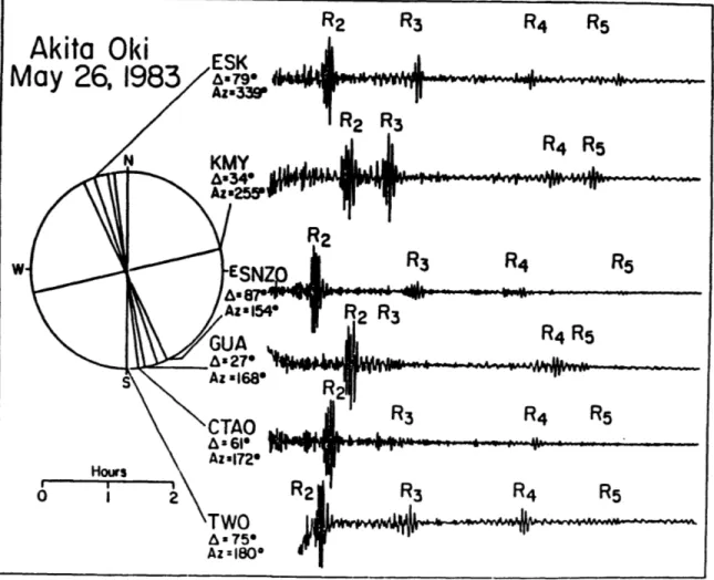
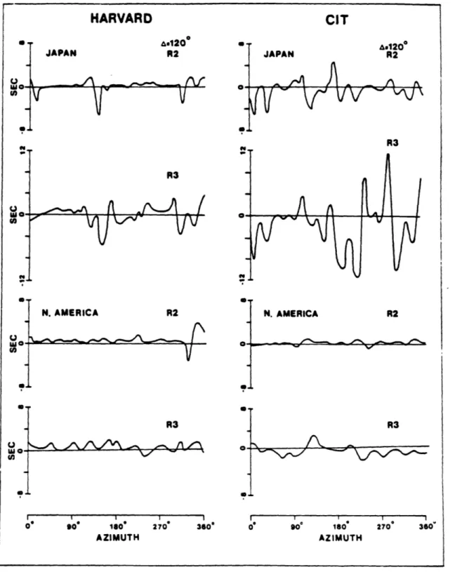
Even for surface waves with periods longer than 150 sec for which the effects of lateral heterogeneity have been considered to be small, peculiar amplitude anomalies are sometimes observed. For example, see the anomalous R3/R2 observations (e.g., large R3 energy at station KMY) for the Akita-Oki earthquake on May 26, 1983 given by Lay and Kanamori [19851 (Figure 1.2). These data imply that we can no longer assume that the waves propagate along great circles. In fact, the travel time calculations by Schwartz and Lay [19851 for recent models such as those of Nakanishi and Anderson [19841 and Woodhouse and Dziewonski [19841 show that the travel times along actual raypaths are sometimes longer than those along great circles (Figure 1.3). If this is the case, this is against Fermat's principle (according to which the travel time along the actual ray path is extreme, in this case,

minimum) on which most of the previous studies are hased. Thus, the procedure of measuring velocity along great circles may not be justified. This is why we need to study surface waves based on wave theories in laterally heterogeneous media. Moreover, the amplitude of a propagating wave is determined essentially by the second spatial derivative of velocity, as will be shown below, whereas the phase term depends on the

velocity along the ray even though ray paths are determined by the first spatial derivative of velocity. Therefore, to delineate laterally

heterogeneous structure, methods which incorporate waveforms are considered to be more powerful than those involving only phase terms.

The Earth appears to be strongly stratified vertically, while the horizontal variation in structure is much weaker and usually quite smooth. For such a medium, we may not need to treat the heterogeneity in all

directions equally as in three-dimensional ray tracing. Instead, this study aims at using the concept of ray theory only for the lateral

propagation of normal modes while the vertical structure, assuming lateral homogeneity in the zeroth order approximation, is to he described by the conventional normal mode theory for surface waves. This means that a ray corresponding to a mode characterized by an eigenfunction determined for the local vertical structure propagates horizontally like a two-dimensional

ray of a body wave. This approach is, in fact, not a new one. For

example, long-range, low-frequency acoustic waves propagating in the ocean have been discussed in terms of normal modes in the vertical direction and

by ray theoretical approaches in the horizontal direction for nearly

horizontally stratified media [e.g., Pierce, 1965; Weinberg and .Burridge, 1974]. A good summary of this subject is found in Burridge and Weinberg

[1976]. For seismic surface waves, several theoretical works [e.g., Kirpichnikova, 1969; Gjevik, 1973; Woodhouse, 1974; Rahich et al., 1976; Hudson, 19811 and numerical calculations based on the standard ray theory for realistic Earth models rSobel and von Seggern, 1978; Wong and

Woodhouse, 1983; Lay and Kanamori, 19851 have been performed. However, the standard ray theory requires a two-point ray tracing between source and

receiver. This requirement leads to large computation time and has discouraged wide application of this approach.

recently developed methods, the Gaussian beam approach [eerveny et al.,

19821, to the surface wave prohlem. The Gaussian beam approach is an extension of the paraxial ray approximation, which is based on the standard

ray theory [Ferveny et al., 19771. Tests and applications of the Gaussian beam method to seismology have been conducted by Nowack and Aki [1984al, Cormier and Spudich [19841, MUller [1984], and Madariaga and Papadimitriou [1984].

We first derive the Gaussian beam formulations for surface waves in a laterally slowly-varying medium in Chapter 2. These formulations are for one beam. Then, in Chapter 3 we obtain the expressions for synthetic seismograms by the summation of each Gaussian beam derived in Chapter 2. We point out differences in these expressions between surface waves and body waves obtained in previous studies. In Chapter 4, numerical testing of the methods developed in the previous chapters is conducted by forward modelling of Rayleigh waves for a heterogeneous Pacific Ocean structure. Finally, in Chapter 5, we attempt to reach our ultimate goal: inversion of both amplitude and phase data to obtain laterally heterogeneous structure using the above methods. Rayleigh wave phase velocities in the Pacific Ocean are inverted for comparison with the conventional pure path phase velocity method. The inverse formulations are non-linear following

Tarantola [1984a,b]. The main conclusions and the implications for future

-g SANTA CRUZ I* 1s .17 OCT 1e60 .E. was L0 JCT 10- DAL --0 AM yCA , coZ C G ALO IsCC SANTA CRUZ IS 20 JUNE 1966 aSK 10 AAM ALO. Con soz ' uP J -0~ ~~ ryiL- ~~s uetaa 40 46 60 66 60 AZIMUTH

Figure 1.1. Observed amplitude of about 20 s at stations in

Tonga-Kermadec trench. Note Longmire (LON) and Corvallis

50 AZIMUTH

variations of Rayleigh waves with periods North America for events in the

the large amplitude difference between (COR). Reproduced from McGarr [1969b].

TONGA I& S OCT 1906

'ao oAL

(4rALo AA gA YJATh:

Figure 1.2. Anomalous R3/R2 observations at station KMY for the Akita-Oki earthquake. Reproduced from Lay and Kanamori [1985].

Figure 1.3. The difference in travel times between great circle and actual raypaths for ?00s Rayleigh waves from sources in Japan and North America using recent models at Harvard FWoodhouse and fziewonski, 19R41 and CIT rNakanishi and Anderson, 19R41. Reproduced from Schwartz and Lay

Chapter 2. Gaussian Beam Formulations for Surface Waves

In this chapter, we shall derive the Gaussian beam formulation of surface waves in a laterally-slowly.varying medium. A flat and isotropic model with slight undulations of the free surface is assumed. Our

procedure follows earlier papers on Gaussian beams such as that on seismic body waves by erven' and Plen~k [19831. The main difference in our method is that the variations of medium parameters in the vertical

direction and in the horizontal directions are not treated equally. The vertical variations are assumed to be much more rapid than the horizontal ones, whose ratio is described by a small parameter c<<1. The main

features of the wavefield are followed by surface wave normal mode theory with an averaged vertical structure, and the lateral heterogeneity gives the modulation of such normal modes in a manner similar to two-dimensional ray theory. The final formulations are equivalent to the previous work of Woodhouse [1974], Babich et al. [19761, and Saastamoinen [19841. However, our formulation gives a great advantage over those results because the wavefields can be evaluated not only on the ray hut also in the

neighborhood of the ray in the sense of the paraxial approximation. In this form, it can he naturally extended to the (aussian heam nethod

[ervenj et al., 19821 based on the more complete wave theory. In the derivations of the formulation, we shall assume that parameters of the medium are continuous functions of depth, hut the final results are also valid in layered media whose interfaces have gradual lateral variations.

In section 2.1, the elastodynamic equations are derived for laterally slowly-varying media. The horizontal variations in such media are much smoother than the vertical ones. We shall change the horizontal scales by

introducing one small parameter so that all of the variables are of the same order. In section 2.2, the trial form of the solution based on the asymptotic ray theory is inserted into the elastodynamic equations obtained

in section 2.1. In the leading terms, the component perpendicular to the ray is decoupled from both that along the ray and the vertical component. This means that essentially there are two kinds of waves, Love and Rayleigh waves, as for laterally homogeneous media. In section 2.3, for each one of the above Love and Rayleigh waves, higher order equations are considered. Eventually, we obtain the parabolic equations which have been studied extensively in the literature on seismic body waves. Finally, in section 2.4, such parabolic equations are solved and we obtain two important equations: the dynamic ray-tracing equation and the transport equation. The final forms of the wavefields are then obtained. In section 2.5, we shall interpret the physical meaning of each term in the final formulation.

2.1 Elastodynamic Equations of Motion in Ray-Centered Coordinates The elastodynamic equations of motion in a general orthogonal, curvilinear, right-handed coordinate system El. E2 and E3 with the

corresponding scaling factors hl, h₂ and h3 are given in section 2.6 of Aki and Richards [19801. Neglecting the body force term, the equation of motion may be expressed as

32u -3 3

p W = hI - (p nphlh~h3/hq) (2.1)

3 p=l q=1

_aEq

where u(E1,E2,E3,t) are displacement vectors in the coordinate system Ei, p is density, t is time, Tpq are stress-tensor components, and n is the unit vector normal to the surface Ep = const. We consider only an

isotropic medium, and the stress-strain relation is expressed in terms of two Lame constants X and U:

3

pq = x6pq : err + 2_{pepq (2.2)}

r=1

where

opq

jr

R+~

h

a

u

6

3 u ah(23

epqn = +()] + rT (2.3)

We consider a semi-infinite medium with axes El = x, E2 = y, and 3 = z, in

which the z-axis is directed downward (Fig. 2.1). In the remainder of this section, the medium is considered to be flat and to be described in

Cartesian coordinates. The transformation between spherical and Cartesian coordinates is discussed in Yomogida and Aki [19851 and in Chapter 3.

As we mentioned in the Introduction, vertical structure is treated using normal mode theory, and we consider rays along the surface. For

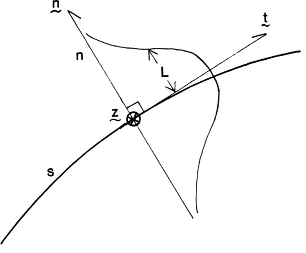
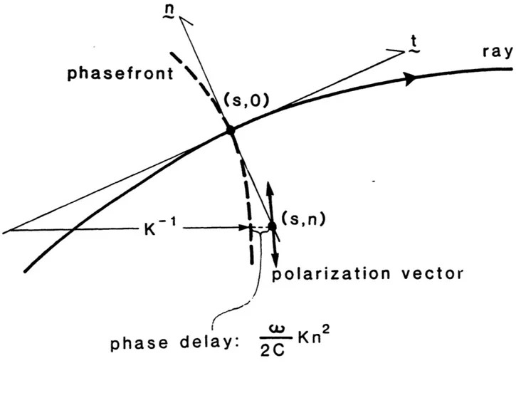
horizontal directions, we introduce ray-centered coordinates (s,n) in the following manner [Popov and Penlik, 19781. The coordinate system (s,n) is connected with the ray as shown in Figure 2.2, where s represents the

arclength along the ray, and n measures length perpendicular to the ray at the point s. On the ray, n is zero. We denote the unit vectors tangent and perpendicular to the ray as t and n, respectively. The remaining

coordinate is the same as the original one, z, which is directed vertically downwards (Fig. 2.1). Thus, we set (g1,&2,E3)=(s,n,z). In this study we assume a medium with weak lateral heterogeneity. We define

nl = S = es, n2 = N = en, n3 = z and T = Et (2.4)

where e is a small parameter. Since the energies propagate mainly along the rays (i.e., along the coordinate S), the time t should be measured with

the same scale as S. In this medium, elastic parameters and density have the following orders:

= 0(1) , a = 0(1) and = 0(1) _{i=1,2,3. (2.5)}

Also, the free surface, z =

C(s,n)

-C. = 0(1) . i=1,2 (2.6)

ani

The medium approaches lateral homogeneity as e + 0 [e.g., Woodhouse, 1974; Babich et al., 1976). The infinitesimal length element dr is represented

in the ray-centered coordinate system by

dr2 = h2dS2+dN2+dz2 (2.7)

where the scaling factor h is given by

h(s,n) = 1 + C-IC n n = 1 + C-IC, N N (?.8)

aC-and the phase velocity C aC-and its first derivative Cn =- for the

corresponding normal mode are evaluated on the ray (at n=n), because alnng the ray the phase front is propagating with the local phase velocity

[C(s,n)ln=0- Fquation (2.7) shows that thp scaling factors hi for the

coordinate system (n10203) = (S, N, z) are

h, = h(s,n), h2 = h3 = 1- (2.9)

Hereafter, we shall consider the wavefield horizontally close enough to the ray for the ray-centered coordinate system (s,n) to he regular [derveny et al., 19821.

may be written as 2 _{E P} 82₈₂ U _*= 1_{-T, -ill} + 12 8h 2 1 +

C

_=~'~

_-TS-'T21

1

E

ell = (X+2p)u + un h + E + X L. bu + u h +a(u2)~ U T22 = h[S un ] + e(X+2) Q + X , 33 =

C

In order to simplify the above equations, we use commas before subscripts to represent the partial derivative with respect to the subscripted

coordinate. For example, us,N = 6u_s/aN, us,TT = 32us/6T2, XS = bA/)S, and

so on. Inserting (2.11) into (2.10), we get

c2p UsTT = eh2Xu)U 5,SS + (ui us , + ch1IX UZzS + ch-lxq~S Uz

+ ch1luz UZ,S),Z + C2h-l(x+u) un,SN + £2h-lrh1(+2i)1S IS,S

1 1 1

+ £21i UsNN + c 2Ans Ufl,S + c 2Asn Us,N + c 2_{Ann Ufl,N}

1 1

+ c2B5 us + £2Bn Uf

e2p Un,TT " e2h?₁u UnSS + Ni Unz, + CA UZ,ZN + uB UZ,N).,Z

+ c2h-l(x+) us,SN + £2h-l(h-luj),S UnS + E2(X+iu) ufl,NN

2A u 4 2 22A2nnu,

+ezz zq + s s~ + c2 Sn us,N+ A2 UN

+ £2B2~ n + £2B2 s US 9 (2.12)

e2P Uz,TT =- e2h-2 uz,SS + U)X+2j)uz z1 z + ch1l+j) usZS

+ ch4lX,z Us,S + cu un ZN + E~ Ufl,N),z + ch jj,S us,z

+ e2ii UZNN + IE2h 4l(h-lu),S UZ,S + eA3 nz unaz

+ C20 zn UzN + cB3~ nUn where A1= h-2 (X+20)h, + h1₁.₁,S + h-lph, Ann = 4 , B s = - h-lUoh,N),N - h-2 Ph,N B n = h-l~hl(x+u)h,N1,s 2 Azz = XN A5 2 h1A= OX h-2(X+3)h, =n hu,.S A = h1 'j, +2phl n N 9hl(x -NNh h-2(x+2₁₁)(h N)2 Bs 9 1h1 hN),9S An 3 h1 (lh),N + h4lxhN Az 9 zn hl(]lh),N Rn (h1 l!N,,z (2.13)

Equations (2.12) give the elastodynamic equations in ray-centered

coordinates.

To consider surface waves (i.e., normal modes), we need boundary

conditions in addition to the above equations. For z + *, displacements must approach zero, that is, the radiation condition should be satisfied:

usun,uz + 0 as z + w . (2.14)

Also, at the surface z=C, any component of traction must vanish;

2

Ti3 - . i 0 (i=1,2,3) at z=c. (2.15)

Using the rescaled coordinate system (S, N, z) and (2.11), the above conditions may be expressed as

y[ch-luz,S + us'zj - e 2 eh-1 (X+2y)u₅ + u

as

+ eXun,N + eD un) - E2!i yE1 = 0 , (2.16a)

3N

gun,z + Cyuz,N - E E2 - eCa F2 = 0 , (2.16b)

Eh"lAugS + (A+2y)uz - Ea UyCh~uzS + us'zl (2.16c)

+ Exun,N + E - E yE3 = 0

where

1 1

D = h-1(X+2u)h,N, E = us,N + h-lun,S- h-lh,N us

E2 = "s,N + h-lun,S + h-1h,Ns '

F2 = Eh-xus,S + eh-1 h,N un + E(X+2p)un,N + Xtz,z (2.17)

D3= h-Ixh,N

3

Using the boundary conditions (2.14) and (2.16), we solve the equations

(2.12) in a manner similar to the solution for a laterally homogeneous

medium in the lowest order of e.

2.2 Laterally Slowly-Varying Approximation For Elastodynamic Equations

For acoustic waves or body waves, it has been assumed that solutions of the elastodynamic equations are concentrated close to rays, or in other words,

"the high-frequency elastic wavefield propagates mostly along rays" [e.g., erveny et al., 1982]. In this study we also seek approximate solutions for propagation along the ray in the direction of increasing s; however the

solutions are expanded in powers of the parameter e which has been introduced to describe the ratio of horizontal variation to vertical heterogeneity

instead of the angular frequency w for body waves [ervenI and Penfk, 1983]. In the present study, the phase term cannot be expressed explicitly as a time-harmonic e-iwt as in the case of body waves or surface waves in a laterally homogeneous medium, because the phase velocity itself varies spatially. Thus, following Woodhouse [19741, we introduce the trial form (ansatz) of the solutions to equations (2.12) as nearly uniform harmonic wavetrains expanded into asymptotic series in powers of e11 :

* k/2 k

uj(s,n,z,t) = ei4(st) Z E Uj(S,N,z,T) j=s,n,z (2.18) k=O

where *(s,t) is the phase advance along the ray. We define wave number k and angular frequency as

k= and W = - . (2.1)

Ray-tracing based on these definitions is slightly different from that for non-dispersive waves [Yomogida and Aki, 19851. We assume that k and w are

slowly varying with respect to s and t:

k = k(S,T) = w(S,T)/C(S) and w = w(S,T) (2.20) where we assume that phase velocity does not vary with time.

To use the asymptotic ray theory developed above, the following

conditions must be satisfied by analogy to the high-frequency approximation [Kravtsov and Orlov, 1980]:

k = 'vy or _p (2.21)

and (2.22)

where t is the characteristic scale length of heterogeneity, ' is the distance from source to receiver, and V₁ denotes the lateral gradient. These conditions mean that the lateral variation of a medium must be small within a wavelength and the receiver must be within the first Fresnel zone.

For surface waves, this means that coupling among different modes can be neglected [e.g., Gregersen and Alsop, 19761. For example, k is -about 0.04 km-1 for 40-sec Rayleigh waves. In oceanic regions a typical value for t may be over 1000 km and the raypath length

iT

Following Babich and Buldyrev [1q721, the solutions concentrated close to a thin 'boundary layer' (the scale of one wavelength) along a ray have a scaling factor N = O(El/2), which is similar to n = 0(w-1/2) of the

high-frequency approximation for hody waves rderven' and Psencfk, 19831. For consistency, the coordinate N should be replaced hy

V = N//c .(

By inserting (2.18) into equations (2.12) with v and neglecting all terms of order higher than 0(c), we get the following equations. Hereafter, we use lower-case characters (s,nt) for (S,N,T):

[pw2 - h-2(A+2p)w2C-2 + a U3] z1/2USl (UsO + + CUs2)

+ iwC-1h-1 [X a + y] (Uzo + CL/ 2Uzi + EUz 2)

+ C1/2iwC-lh-1(x+y)(Unov ₊ c1/2 U nIv)

+ c{2iwpUsoSt + ip awUsO + ih-2(X+2y)C-1 LwUs0_{at as +}

+ iWCl[(2h-2(X+2₁ )U₅0 S - h-2(X+2u)Cg₅C1IU₅O + h1h1X2)9UO

+ h-1(AUz 0,z),s + h-(UUzo s)tz + yUs0₉vv + iwC-lAnsUn}

[p2 - h-2p2C- 2 + y ] (0 + C1/2Un + 2)

+ el/ 2

{iWc-lh-1(x+y)(UsoIV

+ (X A- + 31 y) (Uz0 + e:1/2 Iz ,v)} az az 9vzA + e{ZiwpUn0,t + ip -L- U 0 + ih-24C- 1 as n0

+j~iwpn

i-

at n

h

s

+

+ (X+2y)Unovv + iwC- 1Ass 2USO + Azz 2 Uzo z} = 0 ,2

(2.23)

[pW2 _{- h-2p} 2_{C-2 + I (X+2p) '] (Uz}0 _{+ Cl/}2_{Uzi + eUz}2₎ + iwC-lh-1

[L

.--

az az

+ e{2iwpUzO t + ip U0 + ih-2PC-l 3 U0

9 at zas

+ i1aC-l[2h- 21pU zs - h-2P CsC-Uz0 + h-'(h-ly)g,sUz0]

+ yaUz0,vv + h-1 (xUsOs),z + h-1 (yUsOz),s + Anz 2 _{U n ,z + Bn}3_Un

_}

0 . _(2.24c)

Equations (2.24) together with (2.18) and (2.23) describe solutions in asymptotic forms.

Similar expansions should he applied to the boundary conditions at the free surface (16). Taking the order only up to 0(e), the results may be written as

y[iwC-1h-1(Uz0 + el/2Uzi + £1z2) + (UIso,z + e/2 Is9z + 2,z))

+ e{h-lIUZ0 - - [iwC--1 (X+2y)U0 + XUz0_,z)

- i C-Ih-lyn } = 0 , (2.25a)

an 1 iJ nw~0

y(Uno,z + CI/ 2Un ,z + EUn 2 ,z) + el/ 2 (j zv + 6l/2UzI v)

- £ { _as yiwC-lh-1 Uno + 3C [XiwC-lh-IUs0 + =Uz",z]} 0 , (2.25b)

an

[iwC-lh-lx(Uso + C1/2Us1 + £Us2) + (X+2u)(Hz ,z + eI/ 2Uzi z + £Uz 2,z)]

+ el/2_{x(Un0v + 1/2 I}

+ e[h-IXUs0 _,s

-p (iC-lh-lIUzO + USO+z) + hih nxUn 0 - yn ,z

(2.25c) = 0

at z = c.

Now the problem is to solve equations (2.24) under the boundary

condi-tion (2.25) and the radiacondi-tion condicondi-tion that Uj + 0 (j=s, n, z) as z +..

2.3 Parabolic Equations for Surface Waves

We now discuss equations (2.24) with boundary conditions at the free surface (2.25) in order to get solutions concentrated close to rays which propagate with the local phase velocities of Love and Rayleigh waves. Then we obtain the parabolic equations which give the dynamic ray-tracing

equations and transport equations. We shall find that the former are exactly the same as those for body waves or acoustic waves [eerveny et al., 1977;- erveny and Hron, 1980] and the latter are equivalent to those given by Babich et al. [1976] or Woodhouse [19741. In equations (2.24), the terms of order unity are equivalent to the characteristic equations of Love waves (for UnO in equation (2.24b)) and Rayleigh waves (for UsO and Uzo in equations (2.24a) and (2.24c)) in a laterally homogeneous medium. Thus, under the assumption of this study (i.e., laterally slowly-varying media) there are two types of surface waves: Love and Rayleigh waves which are decoupled to the first order approximation. Each is discussed

individually. a) Love waves

The non-vanishing component of the displacement vector for Love waves is normal to the raypath along the surface in the zeroth-order

approximation. The zeroth-order solution has neither the component tangent to the ray nor the vertical one. Thus, we shall consider the component tin as a "principal component" [erven' and Plenlik, 19831.

that for Love waves in the local vertical structure at (s,n) (hereafter referred to as a local Love wave). This means that component On must satisfy the characteristic equations of local Love waves (see section 7.2

of Aki and Richards, 1980):

where CL( should ta

[p02 - U462 CL- 2(s,n) + a

]

C(s) = CL(s,0).

26)

(2.27) Then, CL(sn) is written in a Taylor series expansion in n as

CL(s,n) 2 C(s) + Cn(s) n +-1 C,nn(s)n2 a C L ~ s ~ n 2ans~C ( s where (2.28) C S) CL(s~n) C 2 CL(-Sn) an

In=0'

With (8), it is easily shown that

h-2 C-2(s) = CL-2(s,n) + C-3(s) Cnn(s)n2 and

h-1 C-1(s) = CL-1(s,n) +

$

Thus the leading term of order unity in (2.24h) may he written as:

[P2

_[(

]U

_+i-.

In equation (2.30), the coordinate v is used instead of n because, in the vicinity of the ray, v is of order unity from the boundary layer

assumption (2.23). The Taylor series expansion (2.28) in n = el/2v is in fact consistent with the expansion of each component by el/2, as in (2.18).

As shown in equation (2.30), the first term of (2.24b) is not of order unity but of order r.

The terms of order unity in equations (2.24a) and (2.24c) are in fact the characteristic equations for "local Rayleigh waves" except for the appearance of the Love wave velocity. Unless the phase velocity of Love waves is identical to that of Rayleigh waves, which is rarely the case, Uso

and Uzo must vanish in order that these terms be zero:

15so = 11z0 = 0 (2.31)

With (2.30), the terms of order E1/2 in equations (2.24a) and (2.24c) are in fact written as

iwCL-1(x+y)Uno,v +

[pW

.L]Us1

=0 (2.32a)

[y +

X]Uno,v

[pW

=0 (2.32b)

Differentiating Un in (2.26) with respect to v and substituting into (2.32a), we get

[p2C, 2_{CL CL}2 _3z+U azz _ZX(+ 9 + iWCL~I0sl) iwLUj + [X -I- + 9UZy

]uz

[p2

{

These are characteristic equations for local Rayleigh waves with Love wave phase velocity. Using the same argument which led to (31), and putting CL ~ C,

UZ1 = 0 and Un 0 v + i C-Us = n , (2.34)

that is,

Us is the "additional component" in the terminology of eerveny- and Plenlik [19831; it is of higher order than the principal component lin by C1/2 and related to the deviation of the real wavefield from the plane wave

perpendicular to the ray path. _{It is reasonable that there is no Uz} component under the above approximation because rays should propagate only horizontally.

Now let us return to the equation for the principal component Un in (2.24b). The term of order El/2 vanishes because of (2.31). Substituting (2.31) and (2.34) into (2.24b), the next term of order e may be written as

2iukUnO,s + iak Un0 _{+ ipskUn}0 _{+ [Un} 0_{,vv - U(}2_C-3_CnnV2_Uno

+ 2ipwUn 0t + ip UnL = 0. (2.35)

This is the parabolic equation for the principal component Un0_.

The boundary condition at the free surface z=g for local Love waves is (see section 7.2 of Aki and Richards (1980))

aUn

= 0. (2.36)

Thus, in equation (2.25h), the first term should disappear. From (2.31), and (2.34), the most dominant term is of order E, which is

ik

$

This condition will be used later to obtain the transport equation for Love waves.

b) Rayleigh waves

waves are tangent to the ray path along the surface and vertical to the surface in the zeroth order approximation. Thus, components Js and l1z are to be the principal components and Un the additional component. As in the case of Love waves, we take the phase velocity C in equations (2.24) to be the velocity of Rayleigh waves in the vicinity of the ray. That is, in the zeroth order approximation, the components Us and Uz must satisfy the

characteristic equations of local Rayleigh waves:

[m2 - (x+2ya)W2CR-2 + a L]Us + iwCR-1

[X

p2 - yw2CR-2 + -(x+2)

]Uz

3z 3Jz +z (2.8X

where CR(s,n) is called a local phase velocity of Rayleigh waves. Using the analogy of Love waves, C(s) is related to CR(s,n) as in equations

(2.27) and (2.28), replacing the subscript L with R.

Now, let us consider the terms of the zeroth order in equations (2.24a) and (2.24c). With (2.29) (CR instead of CL) they are reduced to

[

[pW2 - (X+2y)w 2{CR- 2 + C-3Cnnn2}

a a L]Us + iw{CR-1 + C2 nnn2}[ _{+ Uz}

-(x+2y)w 2_C-3_{C nnn}2_{Us +}

C-2Cnnn2 [X

A

~' n s 2 3z 3z

e{-(X+2y)w2C-3Cnnv2tUs + - nC332Cn +z (2.39a) and

e{-yw2C-3Cnnv2Jz + C-2r

nnV

_[

than order unity.

The terms of order unity in equation (2.24b) constitute the

characteristic equation for "local Love waves", hut with Rayleigh wave phase velocity. Ry similar arguments in the case of Love waves, Ino must vani sh:

Un0 = 0. (2.40)

Then, the leading term of order e1/2 may be written as

iwCR-1(x+y)Us09v + [X 3 + - ,] + [pW2 - ym2C-2 + Uz]Un = 0.

(2.41) By differentiating (2.38a) with respect to v, we obtain the following from

(2.41):

[p2 - IJW2CR- 2 + a _{az 3 Un' +iw-ICRUs}n + i- 0

9 .]1 = 0. (2.42)

The operator in (2.42) is that for the characteristic equation for Love waves, so putting CR ~ C,

Un' + iw-1CRIsO,v = 0

that is,

On

2-E

Likewise, the terms of order E1/ 2 in both equations (2.?4a) and (2.24c) vanish and the leading terms of order E are now

?i(X+2i)ktls ,s + i(x+2yj) 1- _asUso + i(X+2),kus 0 + ( sVV

- (X+2y)w2C-3C,nnv2Us0 + [x L zC-2Cnnv2 + a y]Uz0

++ + 2pnnn + ip UsO = 0 ,

+

(XUZ

_(iUZ

(2.43)

2igktizOs + iy UzO + iuskUz0 + IUzv - ii 2_C-3_Cnnv2_{UzO +}

+ fC-2Conn2 [y + ]Us + (yUs ,z), + (XUs0,s),z

- iCM-[y1

L

X]Us,vV

Equation (2.43) shows that the additional component Un is coupled to only one of the principal components Us. The behavior of Uz is independent of

Un and is determined only from the local vertical structure along the ray and not from neighboring structure, within the accuracy of the above approximation.

Now let us find the boundary conditions at the free surface z=c. For

Rayleigh waves the boundary conditions are shown to be different from those in the laterally homogeneous medium while they are the same for Love waves (2.36). The boundary conditions at the surface for local Rayleigh waves

are written (see section 7.2 of Aki and Richards, 1980):

iwCR-(sn)Uz + Isz = 0 ,

(2.45)

(X+2y)Uzgz + )iwCR-1(s,n)Us = 0

with CR(s,n) the local phase velocity. Using (2.29), the terms of order unity in equations (2.25a) and (2.5?c) are of order e but not of order unity like the terms in (2.39). Then, the largest contribution comes from the terms O(e) in (2.25a) and (2.25c), which are

'A C-2Cnnv2Uz0 + yUJz09s -

{C

i C-2,v2Us0 - ik-IUsOv + xJs ,s - L (i C-luz + ,z) = 0

~ 2 nnIsO 91 0 s as UOC 1O + tJsO~z

(2.46) 2.4 Solutions of Parabolic Equations

For both Love and Rayleigh waves we obtained parabolic equations (2.35) and (2.44) with the boundary conditions (2.37) and (2.46). Although there are several differences between them and the parabolic equations for

acoustic waves [erveny et al., 19821 or for elastic body waves Feerveny and Pencik, 1983] (especially for Rayleigh waves, because of the coupling between components Us and Uz), we solve them by similar procedures.

a) Love waves

Following Babich and Kirpichnikova [19743, we assume solutions of the form

Uno = A(s,t)xl(s,z) exp[ W(s,t)v2M(s)] (2.47)

where ti(sz) is an eigenfunction of the local Love wave at a point (s,n=O) (same notation as in section 7.2 of Aki and Richards F1980~) which is normalized as t1=1 on the surface, and A(s,t) and M(s) are complex-valued

scalar functions. Note that we assume that M is not a function of t.

Substituting (2.47) into (2.35) yields

i[2yk(A11),s + P _as At₁ + ysk At, + wMyAzi + 2wpA,til + -L _at pAti]

(2.48)

We multiply (2.48) by At and integrate with respect to z from the surface c(s) to *. For convenience, we define the following energy integrals (see

section 7.3 of Aki and Richards [19801),

Ii(s) =

f

(2.49) 1

12(s) =

f

c(s)

Using integration by parts, equation (2.48) may be written as

i{ (kA 212) + wMA212 + - (wA2I,) + k U(At)2 yC z

(2.50)

- v2A2[wkI₂(Ms + CM2 + C-2C nn) + M(k1₂ aw + W1₁ )] -- 0.

From boundary condition (2.37), the term evaluated at z=C in (2.50) should vanish. Because the group velocity U is expressed by the energy integrals as

H = 1₂/C1₁ (2.51)

(see equation 7.70 in Aki and Richards [19801), equation (2.50) may be written as

i{L (wA21) + (UwA 21i) + CIJwMA2 I1}

(2.52)

- v2A2wIi[k(M's + CM2 + C-2C nn) + M(-- + H )] = 0.

Let us define the length of ray path as ds=udt (see Chapter 3). Since

+ U = 0. (2.53)

at

Thus, for the left-hand side of (2.52) to be zero for any value of v, it is clear that

(wA2_{I) + (lwA} 2_{Il) + C[IwMA}2_I

1 = 0 (2.54)

and

M,s(s) + C(s)M2(s) + C-2(s) Cnn(s) = 0 (2.55)

The above equations deal with only the lowest-order solution like link with k=0. In general , we might consider a solution with an infinite system for kyl. Babich and Kirpichnikova [19741 and Klime [19831 showed that general solutions of order k are represented by k-th order Hermite

polynomials: these solutions are called Hermite-Gaussian beams. Here only the basic mode with k=0 will be discussed; higher modes are neglected.

Equation (2.55) is similar in form to the dynamic ray tracing equation for acoustic waves or elastic body waves. It has the form of a first order non-linear ordinary differential equation with respect to s of the Ricatti type and can be transformed into two linear differential equations. Let us introduce new complex functions q(s) and p(s):

M(s) = 1 dq(s) p(S) (2.56)

- C(s)q(s) ds ~

qTs).

Then, equation (2.55) nay he written as a system of two linear ordinary differential equations: A = C(s)p(s) , ds (2.57) = - C-2(s)Cnn(s)q(s). ds

We may solve the differential equations (2.57) along the ray to get p and q at any point on the ray. The above procedures are followed to evaluate geometrical spreading in the conventional ray method [e.g., erveny et al.,

1977; Popov and Pen1k, 1978; eerven' and Hron, 19801. Using (2.54) and the fact that q does not depend on t, equation (2.56) may be written as

a (A2_{qI) +}

-L (UA2qIl) = 0. _(2.58)

at a

Like the continuity equation of fluid mechanics, this equation means that A2qIiU = constant along rays *L- (2.59) That is, the energy flow along the vertical column beneath the

two-dimensional ray tube on the surface is constant because q(s) represents the horizontal geometrical spreading. The energy propagates along the ray

not with the phase velocity but with the group velocity, and i(s') denotes the vertical energy profile. *L is a complex constant along the ray but may differ for different rays and is a function of the azimuth of the corresponding take-off angle.

1 0 0

By inserting equations (2.34) (Us = iw-C[n,v = - CMvIJn), (2.47), (2.56)

and (2.59) into (2.18) and transforming to the original coordinates (S + s, N + n, T + t) (note that M should be also rescaled because of the term ds in (2.56)), the final form for Love waves may be written as

__ __ L__ _

[

u(s,n,z,t) = q s(s)

[n

(2.60) -exp i [*(sgt) + A ' (S n2]

with = -w and a= k = - The function ti is an eigenfunction on the

at as

rays for local Love waves in the same sense as for the laterally

homogeneous medium.. Note that there is no vertical component. When the variables p and q are real and on the ray (n=0), the results are equivalent to those in the ray method [Babich et al., 1976; Woodhouse, 19741.

b) Rayleigh waves

As in the case of Love waves, we assume solutions of the form

Us0 = A(st)rl(sz)exp(j Wv2M(s))

(2.61) UzO = A(s,t)ir2(s,z)exp( 2v 2M(s)).

We put the imaginary unit i in Uz0 because there is a w/2 phase difference between horizontal and vertical displacements for Rayleigh waves. The eigenfunctions r, and r2 correspond to those in section 7.2 of Aki and Richards [1980], normalized so that r2=1 on the surface. Substituting

(2.61) into (2.44) gives

i{2(A+2p)k(Ari),s + (X+2y) -k Ar1 + (x+2y),skAri + (X+2y)wMAri

as

(XAr2,z),s + [U(Ar₂),s),z + 2atA,tr1 + pAr₁}

- v2A{(A+2y)r₁[k(wM),s + W2M2 + w2C-3Cnn]

+ [(WM),s + wC-2_{C nn][x a + { yj]r}

i{2uk(Ar₂),s + U a Ar₂ + PskAr₂ + yiMAr 2 - (uArl,z),s

[X(Ari),s),z - CMA[i + 2-

X]rj

- v2A{yUr ₂[k(M),s + W2M2 + W2C-3Cnn]

- ~[(M),s + C-2C nn + 2wCM2][y a + - x]rl + w .L MpAr2}

Then we multiply (62a) and (62b) by Ar₁ and Ar₂, respectively, integrate them with respect to z from ; to w, and sum the two equations. Now we define the following energy integrals (see section 7.3 of Aki and Richards [1980]), Ii(s) = 21 12(s) 2

f

f

f

Using integration by parts and the radiation condition (2.1a), we get

i{-L [A2(2kI ₂ + 13)] + CMA2(2kI2+I3) + 2 (wA 2 1 ₎ - jart)] - A2[k((A+2y)rl2+y r22)-(r 2) ar_az2 + CMA2_Arir 2 z= ₊ - 2 az a s - pr1( Ar2) ,s] = _0. (2.62b) (2.63) + A[XA( Arl) ,sr2

- v2_A2

_{w(2kI

Next we consider the boundary conditions at the free surface z=C. Inserting (2.61) into the two equations of (2.46), multiplying by r, and r₂, respectively, and summing these two relations, we see that the terms evaluated at z=C in equation (2.64) vanish. Also, using the equation for group velocity (equation 7.76 in Aki and Richards F19801),

U= (2k1₂+13)/2wll , (2.65)

equation (2.64) becomes identical to equation (2.52) for Love waves. Thus, with definition (2.53), we get both the dynamic ray tracing equations

(2.57) and the transport equation (2.59). We shall denote the constant in (2.59) by OR in this case.

Finally, transforming back to the original coordinates, the vertical and horizontal components of Rayleigh wave displacement may be written as

OR np(s)C(s)

u(s,n,z,t) = [rl(s,z)(t + (s) n) + ir2(s,z)z

exp i [ (s,t) + n2

]

where r, and r₂ are eigenfunctions on the ray (s,O) for local Rayleigh waves.