Approach for assessing the climate resilience of buildings to the effects of hygrothermal loads

(1)

https://doi.org/10.4224/23003982

READ THESE TERMS AND CONDITIONS CAREFULLY BEFORE USING THIS WEBSITE. https://nrc-publications.canada.ca/eng/copyright

Vous avez des questions? Nous pouvons vous aider. Pour communiquer directement avec un auteur, consultez la première page de la revue dans laquelle son article a été publié afin de trouver ses coordonnées. Si vous n’arrivez pas à les repérer, communiquez avec nous à PublicationsArchive-ArchivesPublications@nrc-cnrc.gc.ca.

Questions? Contact the NRC Publications Archive team at

PublicationsArchive-ArchivesPublications@nrc-cnrc.gc.ca. If you wish to email the authors directly, please see the first page of the publication for their contact information.

NRC Publications Archive

Archives des publications du CNRC

For the publisher’s version, please access the DOI link below./ Pour consulter la version de l’éditeur, utilisez le lien DOI ci-dessous.

Access and use of this website and the material on it are subject to the Terms and Conditions set forth at

Approach for assessing the climate resilience of buildings to the

effects of hygrothermal loads

Lacasse, M. A.; Defo, M.; Gaur, A.; Moore, T.; Sahyoun, S.

https://publications-cnrc.canada.ca/fra/droits

L’accès à ce site Web et l’utilisation de son contenu sont assujettis aux conditions présentées dans le site LISEZ CES CONDITIONS ATTENTIVEMENT AVANT D’UTILISER CE SITE WEB.

NRC Publications Record / Notice d'Archives des publications de CNRC: https://nrc-publications.canada.ca/eng/view/object/?id=757e8bd5-90f3-4656-997f-3ac547fa66ec https://publications-cnrc.canada.ca/fra/voir/objet/?id=757e8bd5-90f3-4656-997f-3ac547fa66ec

(2)

Approach for Assessing the

Climate Resilience of Buildings

to the Effects of Hygrothermal

Loads

M. A. Lacasse, M. Defo, A. Gaur, T. Moore, and

S. Sahyoun

CRB-CPI-Y2-R18

June 30, 2018

(3)

(4)

of Buildings to the Effects of Hygrothermal Loads

Author

Dr. Michael A. Lacasse

Approved

Philip Rizcallah, P. Eng. Program Leader

Building Regulations for Market Access NRC Construction Research Centre

Client Report:

CRB-CPI-Y2-R18

Report Date:

30 June, 2018

Contract No:

A1-012020-05

Reference:

29 November 2016

Program:

Building Regulations for Market Access

42 Pages 3 of 3 copies

This report may not be reproduced in whole or in part without the written consent of both the client and the National Research Council of Canada

(5)

(6)

List of Figures

Figure 1: Projected change in total precipitation in April and mean temperature in June for the period of 2051-2080; information is relative to a 30 year baseline between 1976-2005; assumed climate change scenario: RCP8.5... 2 Figure 2: The climate moisture index under different climate scenarios and timeframes; RCP8.5 assumes

climate change scenario of continued increases in GHG emissions; RCP2.5 rapid GHG

emissions reductions... 3 Figure 3. Climate Zones of Canada and corresponding Köppen climate classification... 9 Figure 4: Sectional view of the different wall assemblies to be evaluated through hygrothermal simulation..11 Figure 5. Boxplot of historical (H) and future (F20 and F35) climate parameters in Ottawa. F20 & F35

respectively represent the scenarios of 2.0 and 3.5 increases in temperature...21 Figure 6. Boxplot of historical (H) and future (F20 & F35) climate parameters in Niagara Falls. F20 & F35

respectively represent scenarios of 2.0 & 3.5 increases in temperature...21 Figure 7. Boxplot of historical (H) and future (F20 and F35) climate parameters in Thunder Bay. F20 & F35 respectively represent the scenarios of 2.0 and 3.5 increases in temperature...21 Figure 8. Comparison of historical mean annual temperature in Niagara Falls, Ottawa and Thunder Bay.

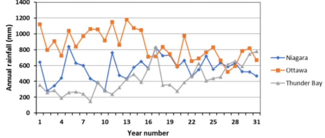
Year number 1 corresponds to the year 1986 and year number 31 corresponds to 2016...22 Figure 9. Comparison of historical total annual rainfall in Niagara Falls, Ottawa and Thunder Bay. Year

number 1 corresponds to the year 1986 and year number 31 corresponds to the year 2016...22 Figure 10. Comparison of historical annual mean relative humidity in Niagara Falls, Ottawa and Thunder

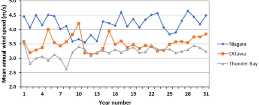
Bay. Year number 1 corresponds to the year 1986 and year number 31 corresponds to 2016...22 Figure 11. Comparison of historical mean annual wind speed in Niagara Falls, Ottawa and Thunder Bay.

Year number 1 corresponds to the year 1986 and year number 31 corresponds to 2016...23 Figure 12. Boxplot of historical & future (F20 & F35) moisture index in Niagara Falls, Ottawa and Thunder

Bay. F20 & F35 represent scenarios of 2.0 & 3.5 increases in temperature, respectively...24 Figure 13. Boxplot of historical & future (F20 & F35) free wind driven rain in Niagara Falls, Ottawa &

Thunder Bay. F20 & F35 represent scenarios for increased temperature, of 2.0 and 3.5...24 Figure 14. Comparison of historical moisture index in Niagara Falls, Ottawa and Thunder Bay. Year number 1 corresponds to the year 1986 and year number 31 corresponds to the year 2016...25 Figure 15. Comparison of historical free wind-driven rain in Niagara Falls, Ottawa and Thunder Bay. Year

number 1 corresponds to the year 1986 and year number 31 corresponds to the year 2016...25 Figure 16. Geometry and meshing of a portion of the horizontal section (top view) of a) W7: brick veneer

and b) walls W1: direct applied stucco, W4: vinyl cladding, and W5A: hardboard siding...30 Figure 17. Moisture storage capacity of the cladding materials. Axis y are logarithmic scale to permit

visualizing the difference between materials. ...31 Figure 18. Liquid diffusivity of the cladding materials. Both x and y axis are logarithmic scales to permit

visualizing the difference between materials. ...31 Figure 19. Vapour permeability of the cladding materials. Both x and y axis are logarithmic scales to permit

visualizing the difference between materials. ...31 Figure 20. Comparison of two methods of selecting reference years based on response of outer layer of

spruce stud for W1 (direct applied stucco) for cities of Ottawa, Niagara Falls, Thunder Bay. ...36 Figure 21. Comparison of the difference between future F35 and historical moisture content for wall W1

(direct applied stucco). The vertical brown line indicates the end of the conditioning year...37 Figure 22. RHT values at outer layer of spruce stud of W1 (direct applied stucco) for historical and future

(9)

CLIMATE RESILIENCE OF BUILDINGS TO THE EFFECTS OF HYGROTHERMAL LOADS

Figure 23. Comparison of differences between future F35 and historical moisture contents of different wall systems for the cities of Ottawa, Niagara Falls and Thunder Bay. Reference years selected using MI method; vertical brown line indicates end of conditioning year. ...39 Figure 24. Comparison of the differences between future F35 and historical moisture contents of different wall

systems for the cities of Ottawa, Niagara Falls and Thunder Bay; Reference years selected using WDR method; vertical brown line indicates end of conditioning year...40 Figure 25. Comparison of difference between future F35 and historical (H) RHT values for different wall

systems for the cities of Ottawa, Niagara Falls and Thunder Bay using a) MI method and b) WDR method...40 Figure 26. Comparison of differences between future F35 and historical moisture contents of different wall

systems for the city of Ottawa...41 Figure 27. Comparison of difference between future F35 and historical (H) RHT values for different wall

systems for the cities of Ottawa, Niagara Falls and Thunder Bay using a) MI method and b) WDR method...41

(10)

List of Tables

Table 1: Climate regions of Canada, representative locations and corresponding selected climate data and Köppen classification ... 8 Table 2 ‒ Climate parameters required for performing hygrothermal simulations in Delphin and steps taken

to prepare them. ...12 Table 3 ‒ Climate parameters available in ‘historical’ climate database provided by Environment and Climate Change Canada (ECCC)...13 Table 4 ‒ Climate parameters available in ‘historical’ climate database provided by UK Met Office. ...13 Table 5 ‒ Solar declination angle and equation of time for the 21st_{day of each month as recommended in}

Hutcheon and Handegord28_{. ...18} Table 6. Yearly values of climate parameters over the reference years selected for Niagara Falls using

moisture index criteria ...26 Table 7. Yearly values of climate parameters over the reference years selected for Niagara Falls using free

wind-driven rain index criteria ...26 Table 8. Yearly values of climate parameters over the reference years selected for Ottawa using moisture

index criteria...26 Table 9. Yearly values of climate parameters over the reference years selected for Ottawa using free

wind-driven rain index criteria...27 Table 10. Yearly values of climate parameters over the reference years selected for Thunder Bay using

moisture index criteria ...27 Table 11. Yearly values of climate parameters over the reference years selected for Thunder Bay using free

wind-driven rain index criteria ...27 Table 12. Characteristics of the three cities selected for hygrothermal simulations. ...29 Table 13. Cladding material, density and thickness...29

(11)

(12)

Summary

Under the Pan-Canadian Climate Change Framework, Infrastructure Canada is providing funding to NRC to deliver the Climate-Resilient Buildings and Core Public Infrastructure (CRBCPI) Project over a 5 year period. The purpose of the project is to develop decision support tools, including codes, guides and models for the design of resilient new buildings and CPI and rehabilitation of existing buildings and CPI in key sectors to ensure that existing and future climate change and extreme weather events are addressed. CRBCPI aims to integrate climate resilience into design guides, codes and related materials which will be the basis for future infrastructure builds and rehabilitation work in Canada.

The CRB-CPI program specifically relating to the Climate Resilience of Buildings (CRB) is to determine the climate resilience of building enclosures. The state of practice relates not only to the effect of climate change on building enclosures, but it is also intended to assess the effect of climate change on the

durability of components of building enclosures.

Two aspects that are to be studied as part of the CRB program focusing on building enclosures (BE): (i) the hygrothermal response of BEs to a changing climate, and; (ii) the overheating of buildings due to urban heat island effects as may arise due to climate change.

The work described in this report focuses on the hygrothermal response and durability of BEs to a changing climate. A review of recent literature on the hygrothermal performance assessment of building enclosures with respect to the assessment of climate change impacts has been completed. Several future climate scenarios have to be considered and uncertainties introduced in analysis in consideration of developing outcomes. None of the existing methods for selecting moisture reference years for hygrothermal simulations produces consistent spatial and temporal climate data results. Risk to water entry of walls will increase in some areas and decrease in others, depending on the change of local climatic variables.

For this fiscal year, hygrothermal simulations were performed to investigate the effects of climate change on the hygrothermal response of four (4) wall systems found in homes and small buildings, typically referred to as buildings conforming to Part 9 of the NBC, in the cities of Ottawa, Thunder Bay and Niagara Falls. These walls have similar configurations inboard the cladding but differ by their cladding materials. Two climate change scenarios (2 and 3.5C) under Representative Concentration Pathways of 8.5 and two methods of selecting the moisture reference years were considered. For hygrothermal simulations, two representative years were selected in each group of weather data in the following manner: the years comprising the chosen time-periods were ranked in increasing order of average magnitudes of moisture index or wind-driven rain and the year ranked 16th (out of the 31 years in each time-period) was chosen as the “average” hygrothermal year and used for wall conditioning. The last ranked year was chosen as the “test” year; this year was the most severe amongst the 31 ranked. The impact of climate change was compared using the moisture content and RHT differences between values obtained using future and current climate data. RHT evaluates the total number of instances in which a location in a wall assembly is above threshold conditions for relative humidity (RH) and temperature (T). The threshold values for this assessment were taken as RH of 80% and T of 5°C. These are conservative values, and represent the potential for onset of mould growth. The moisture source used in the simulations was determined assuming water entry beyond the cladding in the wall system. It was calculated as 1% of

(13)

CLIMATE RESILIENCE OF BUILDINGS TO THE EFFECTS OF HYGROTHERMAL LOADS

the wind driven rain, and was applied to the exterior side of the sheathing membrane, as recommended by ASHRAE 160 Standard.

Simulation results show that the hygrothermal response of building enclosures to future climate varies geographically, with the climate change scenario and with the wall type. The two methods of selecting the moisture reference years yield different responses. These preliminary results suggest that the combined effect of change in climatic variables will lead to a decrease risk of deterioration in some areas and an increase risk in others for the walls studied, and that the response will depend on the emission scenario used to develop climate data. However, further investigations needed to be performed. In fact, there is a need to investigate more cities across the country, other methods of selecting the moisture reference years and as well to undertake water tightness tests under severe wind-driven rain loads and wind pressures to permit estimating the amount of water entry beyond the cladding, and the distribution of water into the wall systems.

(14)

Approach for Assessing the Climate Resilience of Buildings

to the Effects of Hygrothermal Loads

Authored by:

M. A. Lacasse, M. Defo, A. Gaur, T. Moore and S. Sahyoun

A Report for the

Climate Resilient Buildings – Core Public Infrastructure project

Infrastructure and Communities Canada

National Research Council Canada Ottawa ON K1A 0R6 Canada

(15)

(16)

Approach for Assessing the Climate Resilience of Buildings to

the Effects of Hygrothermal Loads

M. A. Lacasse, M. Defo, A. Gaur, T. Moore and S. Sahyoun

1. Introduction

It is generally understood that the climate has been warming globally with more frequent and intense extreme events such as heat waves, droughts, wild fires, snow and ice storms, rainfall leading to flooding, as well as wind and hail storms1_{. A global average temperature increase of 0.85°C was observed from the} historical weather data for the past 130 years1_{. For Canada the temperature increase was double and in} the arctic latitudes2_{the increase was triple. Similar trends have also been observed for long (climate) and} short (weather) term precipitation events (rain and snow fall) and average wind speeds.

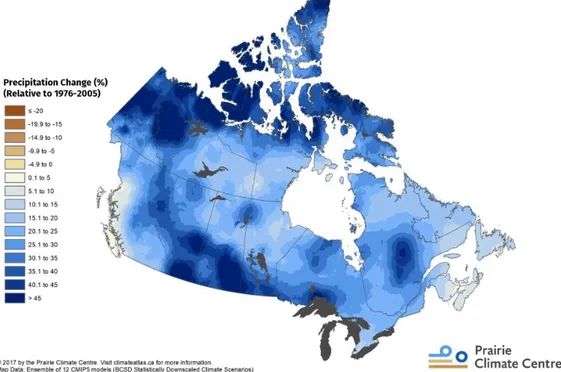
For example, the projected change in total precipitation across Canada in April for the period ranging between 2051-2080 is given in Figure 1. Likewise in the same figure information is provided for the same period for the mean temperature in June. Information in either figure is relative to a 30 year baseline between 1976-2005 and for the RCP8.5 climate change scenario in which it is assumed that there are continued increases in GHG emissions over the years.

As may be seen in Figure 1, there are significant changes anticipated in temperature and precipitation in future years. There is at least an increase of 20-25% in precipitation across all of Canada and in some regions increases in precipitation as high as 40-45% are observed. In respect to the temperature in June, there is projected an increase relative to the baseline of 2-3 °C.

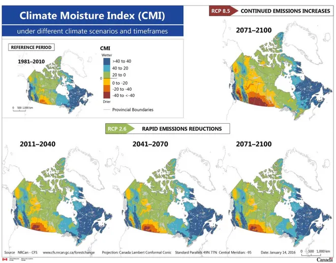
Increases in both of these climate parameters will necessarily affect the climate moisture index, as can be seen in Figure 2 in which the changes in climate moisture index relative to the 30 year baseline period (1981-2010) is shown under different climate scenarios and timeframes. The Climate Moisture Index (CMI) was calculated as the difference between annual precipitation and potential evapotranspiration – the potential loss of water vapour from a landscape covered by vegetation3_{. The RCP8.5 scenario assumes continued emissions increases} whereas for the RCP2.5 scenario, rapid emissions reductions are assumed. It is evident from a review of these maps that the coastal regions and all of Quebec province will experience increases in CMI in future years whereas there will be a marked decrease in CMI for Alberta and the prairie regions.

These changes to the climate will have significant effects on building infrastructures and communities, particularly the durability of building materials, as well as the comfort and health of building occupants. Extreme precipitation events, either snow or rain, may, depending on the severity of the event, increase the risk to inadvertent water entry of wall assemblies potentially leading to their premature failure. It is anticipated that future projections of climate change and extreme events will exacerbate the situation, particularly if the old building stock is not retrofitted to adapt to the expected effects of climate change.

1 IPCC. 2014. Climate change 2014. Synthesis report. Intergovernmental Panel on Climate Change. Geneva, Switzerland; page 151.

2 Bizikova L., Neale T., Burton I. 2008. Canadian communities’ guidebook for adaptation to climate change. First edition, Environment Canada.

3 Hogg, E.H. 1997. Temporal scaling of moisture and the forest-grassland boundary in western Canada. Agricultural and Forest Meteorology 84,115–122.

(17)

APPROACH FOR ASSESSING THE CLIMATE RESILIENCE OF BUILDINGS TO THE EFFECTS OF HYGROTHERMAL LOADS

Figure 1: Projected change in total precipitation in April and mean temperature in June for the period of 2051-2080; information is relative to a 30 year baseline between 1976-2005;

(18)

Figure 2: The climate moisture index under different climate scenarios and timeframes; RCP8.5 assumes climate change scenario of continued increases in GHG emissions; RCP2.5 rapid GHG emissions reductions

Given the expected change in climate in the future and the potential vulnerability of the building stock to such changes, there is interest in determining the hygrothermal response of building enclosures of different building types to the anticipated effects of climate change and from this establishing the relative resilience of the different walls when exposed to loads as may occur in the future. To this end, it is worthwhile reviewing work as has previously been undertaken in respect to the effects of climate change on the building stock, the durability of building components to changing climate loads and the

hygrothermal effects on building enclosures as may arise due to a changing climate. 1.1 Climate change and the hygrothermal resilience of building enclosures

Hygrothermal simulation of wall assemblies is typically used to understand the effects of climate loads on the hygrothermal response of wall assemblies for the purposes of determining the risk to deterioration as may occur from the presence of, e.g., mould, wood rot or other degradation as may occur on assembly components. Whereas a substantial amount of work has been done on the impact of climate change on the thermal performance of buildings, less work has been completed on understanding the effect of climate change on wind-driven rain loads and in turn, on the amount of water that penetrates the outmost layer of façades. Interestingly few hygrothermal studies have been completed on this topic; a brief review is offered on the pertinent literature in this area, and includes work related to climate loads affecting the

(19)

hygrothermal response of building assemblies, the hygrothermal response of attic roofs and different types of wall assemblies.

Climate loads— Nik and Kalagasidis 4_{indicate that undertaking climate change impact assessment of the} built environment is becoming increasingly feasible given the growing knowledge of the process and more importantly, the availability of climate data. However reaching practical conclusions based on such impact assessment studies is a challenge since there are several future climate scenarios that should be considered when completing an assessment. This process, it is suggested, necessarily introduces uncertainties in the analysis which should be a consideration in developing useful outcomes from such studies. Given the warmer and moister climate Sweden is to face in the future as a result of climate change, the authors state that there will be an increased incidence of rain events and as well, the rain events will be more intense. Hence extreme rain events will be more prevalent which will tend to

increase the risks for damage to buildings and the built environment. As a preliminary study on the impact of climate change on wind-driven rain (WDR) loads on buildings, the ASHRAE method was used to calculate the amount of rain deposition on walls, using hourly values of rain and wind data from 6 climate scenarios during the period 1961-2100. Results of this work indicated that the amount of rain deposition necessarily increases in the future, however, as might be expected, there are considerable differences in results induced by climate uncertainties. Further research and numerical simulations of WDR were completed and are summarized in the subsequent section.

In the work undertaken by Nik et al. 5_{the prospective impacts of climate change on wind-driven rain} (WDR) loads were investigated and the resulting hygrothermal performance derived through simulation for common vertical wall construction when subjected to the climatic conditions of Gothenburg, Sweden. The importance of three uncertainty factors of the climate data were investigated and included

uncertainties from: global climate models, emissions scenarios and spatial resolutions. Consistency of the results was examined by modelling walls with different materials and sizes, as well as using two different mathematical approaches for WDR deposition on the wall. The sensitivity of the simulations to wind data was assessed using a synthetic climate with sole wind data. According to the results, it is anticipated that in the future, higher amounts of moisture will accumulate in walls; climate uncertainties can cause variations up to 13% in the calculated 30-year average of water content of the wall assemblies and 28% in its standard deviation. Using sole wind data can augment uncertainties with up to 10% in WDR

calculations, however it is possible to neglect changes in future wind data.

Risk of Frost Damage in Masonry— For the Netherlands under the effects of climate change in the future, it is anticipated that, for the winter months, there will be increases of air temperature and rainfall intensity. As a result, there was interest in knowing whether this would bring about a corresponding increase in the risk of frost damage to masonry. Van Aarle et al. 6_{report on the risk of frost damage to a masonry} wall under climate change conditions. It is supposed that the risk of frost damage might very well increase as a masonry construction may be wet for a longer period of time due to the increase in rainfall events and intensities. Whereas the risk of frost damage may indeed decrease due to the increase in air temperature.

4_{V. Nik, A. Sasic Kalagasidis (2014), Wind Driven Rain and Climate Change: A Simple Approach for the Impact} Assessment and Uncertainty Analysis, 10th Nordic Symposium on Building Physics, NSB 2014, 574-581 5_{V. M. Nik, S. O. Mundt-Petersen, A. Sasic Kalagasidis, P. De Wilde, (2015), Future moisture loads for building}

facades in Sweden: Climate change and wind-driven rain, Building and Environment 93 (2015) 362-375

6_{M. van Aarle, H. Schellen, J. van Schijndel (2015), Hygro Thermal Simulation to Predict the Risk of Frost Damage in} Masonry; Effects of Climate Change, 6th International Building Physics Conference, IBPC 2015, Energy Procedia 78 ( 2015 ) 2536 – 2541

(20)

Accordingly, the research work focused not only on the susceptibility to frost damage of porous materials, but also on the conditions under which material damage occurs, the outside climate conditions conducive to frost damage in the winter period and, the possibility to predicted frost damage with a multi-physical model. Simulations with a hygrothermal model of external building envelopes with the frost sensitive material calcium silicate brick reproduced frost damage as occurs in winters in the Netherlands. The model was used to predict frost behavior in the future under climate change conditions; the outgrowth from this work indicates that there is likely to be a significant reduction in the risk for frost damage under future anticipated climate change conditions in the Netherlands.

Risk of moisture damage / Attic-roof— Nik et al.7_{report on an investigation of the hygrothermal} performance of ventilated attics in respect to possible climate change effects in Gothenburg, Sweden. The focus on attics resulted from an observed increase of moisture related problems (mould growth) over the past 20 years in this moisture sensitive part of the building. Four different attic roof constructions were investigated and simulations were done for the period of 1961-2100 using the weather data of RCA3 climate model downscaling reanalysis data, ERA40, and GCM data, ECHAM5. For the simulation of the future conditions, the hygrothermal response of these different attics was determined from three emissions scenarios: RCA3-ECHAM5-A2, A1B and B1. The mould index and its growth rate were considered as criteria for comparing the hygrothermal performance of these attics.

Based on the results of simulation, the highest risk of mould growth was found on the north roof of the attic. Results point to an increase of the moisture problems in attics in future. It was found that the different emissions scenarios do not influence the risk of mould growth inside the attic due to compensating changes in different variables. According to the simulation results, temperature and humidity levels will increase in the attics upon the onset of climate change effects and this in turn may increase the risk of mould growth in attics located in Gothenburg. Assessing the future performance of the four attics shows that the safe solution is to ventilate the attic mechanically. Insulating roofs of the attic can decrease the condensation on roofs, but it cannot considerably decrease the risk of mould growth on the wooden roof underlay.

Risk of moisture damage / Wood-frame walls— Worldwide efforts toward energy consumption reduction in building sector is one of the areas affected by climate change. Building regulations demand the building construction industry to be more energy efficient. Several studies, the authors8_{mention, have been carried} out on the thermal performance of energy efficient buildings under future changing climates, whereas studies on the durability of energy efficient building envelopes in future climates are rather limited. The authors describe a study to assess the impact of future climates in the Montreal region on the durability of typical Canadian residential wall assemblies retrofitted to PassiveHaus configurations. The assessment considered current (2015), as well as climatic conditions of 2020, 2050, and 2080. The durability performance was evaluated in terms of the frost damage risk to brick masonry cladding and the risk of biodegradation of plywood sheathing within the wall assembly through simulations using the WUFI Pro simulation program. The future weather files were generated based on weather data recorded at the Montreal International Airport weather station using a General Circulation Model HadCM3 based on the A2 emission scenario as provided by the Intergovernmental Panel on Climate Change. The results from this study

7_{Nik, V. M., Kalagasidis, A.S., Kjellström, E. (2012), Assessment of hygrothermal performance and mould growth risk} in ventilated attics in respect to possible climate changes in Sweden, Building and Environment 55 (2012) 96-109 8_{A. Sehizadeh, Hua Ge (2016), Impact of future climates on the durability of typical residential wall assemblies}

(21)

indicated that upgrading wall assemblies to the PassiveHaus recommended level would increase the risk to frost damage of bricks, whereas, this risk would diminish under 2080 climatic conditions. While the decay risk of the plywood sheathing would decrease, the mould growth risk defined by RHT criteria would increase over future climates. Under future climates, mould growth risks of the plywood defined by the mould growth index exist only when rain leakage is introduced and would likely decrease for a double-stud wall assembly.

Nik9_{used synthesizing representative weather data of future climate to undertake impact assessments of the} energy usage efficiency of buildings in climate change conditions using simulation. In a similar manner, this approach was extended to the application of corresponding weather data sets for the hygrothermal simulation of buildings, specifically, a pre-fabricated wood frame wall. To investigate the importance of considering moisture and rain conditions when creating the representative weather files, two additional groups of weather data were synthesized based on the distribution of the equivalent temperature and rain. Moisture content, relative humidity, temperature and mould growth rate were calculated in the facade and insulation layers of the wall for several weather data sets. Results show that the synthesized weather data based on the dry bulb temperature predicts the hygrothermal conditions inside the wall very similarly to the original RCM weather data and there is no considerable advantage in using the other two weather data groups. As such, the study helps confirm the applicability of synthesized weather data based on dry bulb temperatures and emphasizes the importance of considering extreme scenarios in the calculations. This enables having distributions more generally similar to the original RCM data whilst the simulation load is significantly decreased.

Summary— Impact assessments of brick masonry cladding, or wood frame wall and attic roofs have been described using a common approach whereby the response of the structures to anticipated climate loads under different scenarios is determined and resulting effects on the components ascertained. The climate resilience of these structures was evaluated in comparison to results from simulation using historical climate date sets. The work described above suggests that impact assessments of wall component performance when subjected to anticipated climate change loads as may arise in the future under different climate scenarios can readily be established provided suitable hourly data sets have be developed from GCM or RCM or other climate models.

1.2 Climate Resilience of Buildings project

The CRB-CPI program specifically relating to the Climate Resilience of Buildings is to determine the climate resilience of building enclosures. The state of practice as described in Lounis et al.10_{, relates not} only to the effect of climate change on building enclosures, but it is also intended to assess the effect of climate change on the durability of components of building enclosures.

Two aspects that are to be studied as part of the Climate resilience of Buildings program focusing on building enclosures (BE): (i) the hygrothermal response of BEs to a changing climate, and; (ii) the overheating of buildings due to urban heat island effects as may arise due to climate change. The work described in this report focuses on the hygrothermal response and durability of BEs to a changing climate. There are secondary effects that must be considered when implementing

9_{V. M. Nik (2017), Application of typical and extreme weather data sets in the hygrothermal simulation of building} components for future climate – A case study for a wooden frame wall, Energy and Buildings 154 (2017) 30–45 10_{Z. Lounis et al. (2017), Climate Change Adaptation of Buildings and Core Public Infrastructure Summary of}

(22)

resilient (CR) design to the building enclosure. Any changes to the way buildings are built to

accommodate CR design will also need to consider other factors, e.g.: durability, energy use, buildability, and embodied GHGs.

Building enclosures conforming to Part 5 as well as Part 9 of the NBC are implicitly considered in this work program. In respect to hygrothermal loads, this implies that air leakage is considered as part of the hygrothermal response and in which instance, the hygrothermal response is also intended to permit assessing the risk to condensation of the assembly. As such, when the hygrothermal response is assessed, this has implications in respect to the durability, or the long-term performance of the assembly. The primary intent for determining the hygrothermal response and climate resilience of building

enclosures (CR-BE), is to provide information that will then permit developing guidelines for the design of BEs to achieve climate resiliency for both new and existing buildings and guidelines to ensure resiliency by providing a design guide for the durability of BEs. Such guidelines are intended to provide the necessary technical information in support of future updates of the National Building Code of Canada.

2. Approach

The climate resilience of buildings when subjected to the effects of hygrothermal loads acting on the building enclosures is to be assessed though a rigorous review of the response of different types of wall assemblies to climate loads as may occur across Canada. Accordingly, the different regions of Canada for which information on the hygrothermal response of wall assemblies is being sought must be identified as well as the different types of walls assemblies commonly in use in Canada.

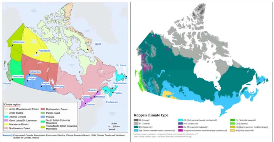
2.1 Climate regions and climate loads

The climate loads are those that occur in the different climate regions of Canada and include at least 8 different regions as provided in Table 1 and Figure 3; the corresponding Köppen climate classification is also provided in Figure 3. In regions where the value of the MI > 1, a capillary break of at least 10 mm is required between the cladding and the backup wall. This capillary break is to help ensure that any water penetrating the exterior cladding towards the interior of the wall assembly has the possibility of being drained to the base of the wall along the entire height of the capillary break and that any moisture that is retained within the drainage area can likewise dissipate through natural convective processes as may occur behind the cladding. This value can nonetheless be very high in the Arctic but is always close to or greater than 1 in more southerly maritime locations; the highest value listed in Table C-2 of the NBC is 4.21 (Ocean Falls, BC) whereas the lowest is 0.23 (Suffield, BC).

Climate loads are to be established for historical and future climates. The hourly climate parameters to be determined for each location include:

 Temperature (°C)  Relative humidity (%)  Horizontal rainfall (mm)  Wind speed (m/s)

 Wind direction (°), from North  Total solar insulation (W/m2₎  Solar diffuse radiation (W/m2₎  Solar reflected radiation (W/m2₎

(23)

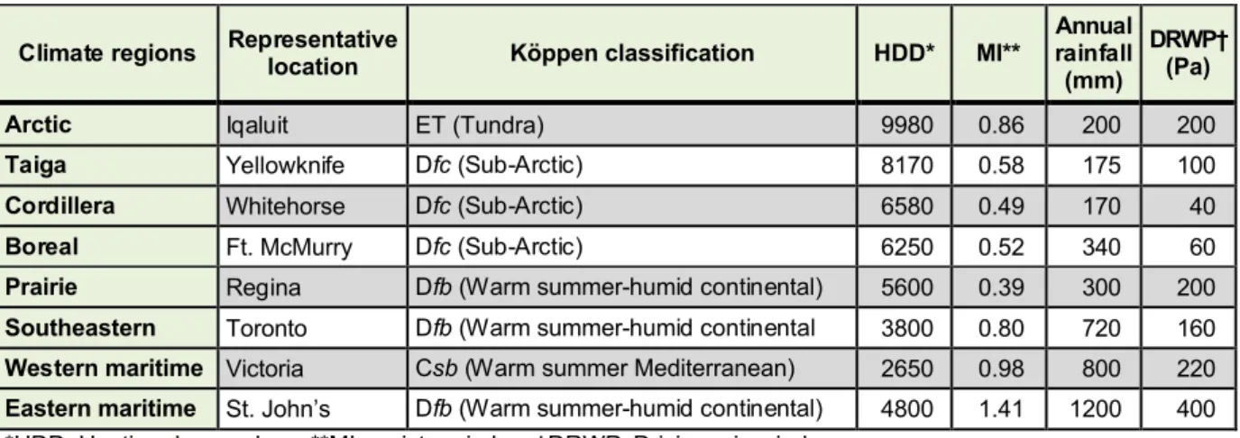
As may be expected, there is a considerable range in the number of HDD across the 8 climate regions, from a high of 9980 HDD in Iqaluit in the Artic to 2650 HDD in Victoria; the colder regions have substantially lower annual rainfall as compared to the warmer regions. The overall risk to the development of possible moisture issues in a wall assembly is given by the MI.

Table 1: Climate regions of Canada, representative locations and corresponding selected climate data and Köppen classification

Climate regions Representative _location Köppen classification HDD* MI** rainfallAnnual (mm)

DRWP† (Pa)

Arctic Iqaluit ET (Tundra) 9980 0.86 200 200

Taiga Yellowknife Dfc (Sub-Arctic) 8170 0.58 175 100

Cordillera Whitehorse Dfc (Sub-Arctic) 6580 0.49 170 40

Boreal Ft. McMurry Dfc (Sub-Arctic) 6250 0.52 340 60

Prairie Regina Dfb (Warm summer-humid continental) 5600 0.39 300 200 Southeastern Toronto Dfb (Warm summer-humid continental 3800 0.80 720 160 Western maritime Victoria Csb (Warm summer Mediterranean) 2650 0.98 800 220 Eastern maritime St. John’s Dfb (Warm summer-humid continental) 4800 1.41 1200 400 *HDD: Heating degree days; **MI: moisture index; †DRWP: Driving rain wind pressure

(24)

(25)

In regions where the value of the MI > 1, a capillary break of at least 10 mm is required between the cladding and the backup wall. This capillary break is to help ensure that any water penetrating the exterior cladding towards the interior of the wall assembly has the possibility of being drained to the base of the wall along the entire height of the capillary break and that any moisture that is retained within the drainage area can likewise dissipate through natural convective processes as may occur behind the cladding. This value can nonetheless be very high in the Arctic but is always close to or greater than 1 in more southerly

maritime locations; the highest value listed in Table C-2 of the NBC11_{is 4.21 (Ocean Falls, BC) whereas the} lowest is 0.23 (Suffield, BC).

Climate loads are to be established for historical and future climates. The hourly climate parameters to be determined for each location include:

 Temperature (°C)  Relative humidity (%)  Horizontal rainfall (mm)  Wind speed (m/s)

 Wind direction (°), from North  Total solar insulation (W/m2₎  Solar diffuse radiation (W/m2₎  Solar reflected radiation (W/m2₎ 2.2 Description of Wall assemblies

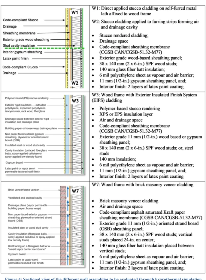
Given that this work focuses on assessing the climate resilience of wall assemblies, a broad range of different types of wall assemblies are those typically designed and constructed in Canada have been considered. This initial portion of the broader study on BE is to emphasize wall assemblies of homes and small buildings, typically referred to as buildings conforming to Part 9 of the NBC. The possible different wall assemblies to be evaluated are all wood frame assemblies that include the following cladding types:

 W1: Direct applied stucco cladding having self-furring lath (regions for MI ≤ 1)

 W2: Code-compliant stucco cladding with furring strips ( i.e. rainscreen in regions for MI > 1)  W3: Exterior Insulated Finish System (EIFS) cladding

 W4: Vinyl siding

 W5: Hardboard siding (with and without furring strips)

 W6: Fibre-cement board siding (with and without furring strips)  W7: Brick masonry veneer cladding

Figure 4 shows the configuration of some of the wood frame wall assemblies. The general configuration inboard of the cladding consists of:

 Sheathing membrane (30 Minute paper, asphalt saturated conforming to CAN/CGSB 51.34-M  Exterior grade wood-based sheathing panel (OSB / 11 mm)

 Wood frame: SPF wood studs (38 x 140-mm / 2 x 6-in.)

 Insulation within vertical stud cavities (glass fibre batt insulation; depth 140 mm)  Vapour and air barrier: polyethylene sheet (6 mil thick)

 Interior grade gypsum panel (12 mm) with latex primer and 1 coat of latex paint

11_{Canadian Commission on Building and Fire Codes (2010), National Building Code of Canada, Volume 2,} National Research Council Canada, Ottawa

(26)

(27)

3 Development of climate data

3.1 Identification of climate parameters required for hygrothermal simulations

A state-of-the-art hygrothermal modelling software, Delphin, was used to undertake the hygrothermal simulations. The time-step for modeling was chosen to be hourly, as the highest temporal frequency climate observations were available at that time-step. Delphin requires climatic parameters listed in Table 2 for performing hygrothermal simulations.

3.2 Collection of raw climate data

Out of the eight climatic inputs listed in Table 2, four (temperature, relative humidity, wind-speed, and wind-direction) were obtained from the ‘historical’ climate database maintained by Environment and Climate Change Canada12_{. The variables available from this database are provided in Table 3.}

Table 2 ‒ Climate parameters required for performing hygrothermal simulations in Delphin and steps taken to prepare them.

S.No. Weather input in Delphin _(shortnames) Units Steps of data preparation

1 Rainfall (RAIN) mm

Precipitation observations from HadISD data  filling-in by CFSR precipitation estimates  conversion of precipitation to rainfall using CFSR categorical rain data

2 Temperature (TEMP) ºC Temperature observations from ‘historical’ and HadISD _{data  filling in by CFSR temperature estimates}

3 Relative humidity (RHUM) % Relative humidity observations from ‘historical’ and HadISD data  filling in by CFSR relative humidity estimates

4 Wind speed (WSP) m/s Wind-speed and wind-direction observations from ‘historical’ and HadISD data  filling in by derived wind-speed and wind-direction estimates from CFSR zonal and meridional wind components

5 Wind direction (WDIR) º from _north

6 Diffuse sun radiation (DHI) W/m2 _{Derived from bias-corrected estimates of NARR}

downward shortwave radiative flux (no filling-in required)

7 Direct sun radiation (DRI) W/m2

8 Atmospheric counter

radiation (ACR) W/m2

Derived from estimates of NARR downward longwave radiative flux at surface values (no filling-in required)

(28)

Table 3 ‒ Climate parameters available in ‘historical’ climate database provided by Environment and Climate Change Canada (ECCC).

S.No. Climate variable Units

1 Temperature ºC 2 Dew-point temperature ºC 3 Relative humidity % 4 Wind speed km/h 5 Wind direction º 6 Visibility km

7 Atmospheric pressure kPa

8 Humidex

-9 Wind chill

-10 Weather

-It was especially noted that precipitation and solar radiation related variables were not available in the above database and therefore other sources of observational data were explored.

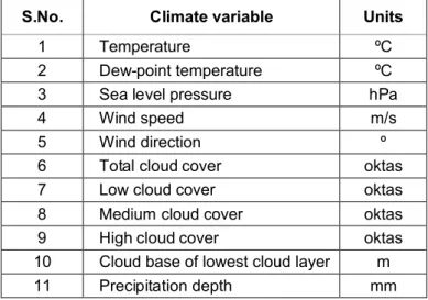
The HadISD datasets13_{maintained by the UK Met office were found to be a reliable source of information} where estimates of climate variables over sub-daily durations of 6 hours or less are provided 14; 15; 16; 17_. The climate parameters that were available from HadISD database are listed in Table 4.

Table 4 ‒ Climate parameters available in ‘historical’ climate database provided by UK Met Office.

S.No. Climate variable Units

1 Temperature ºC

2 Dew-point temperature ºC

3 Sea level pressure hPa

4 Wind speed m/s

5 Wind direction º

6 Total cloud cover oktas

7 Low cloud cover oktas

8 Medium cloud cover oktas

9 High cloud cover oktas

10 Cloud base of lowest cloud layer m

11 Precipitation depth mm

The HasISD database was used to obtain hourly precipitation, temperature, direction, and wind-speeds as they were relevant to hygrothermal modelling in Delphin.

13_{https://www.metoffice.gov.uk/hadobs/hadisd/}

14_{Dunn RJH et al. (2016) Expanding HadISD: quality-controlled, sub-daily station data from 1931, Geoscientific} Instrumentation. Methods and Data Systems 5: 473-491.

15_{Dunn RJH et al. (2014) Pairwise homogeneity assessment of HadISD. Climate of the Past 10: 1501-1522.} 16_{Dunn RJH et al. (2012) HadISD: A Quality Controlled global synoptic report database for selected variables at}

long-term stations from 1973-2011. Climate of the Past 8: 1649-1679.

17_{Smith A et al. (2011) The Integrated Surface Database: Recent Developments and Partnerships. Bulletin of the} American Meteorological Society 92: 704-708.

(29)

As mentioned before, Delphin requires climate variables to be continuous, and devoid of missing values. Observational records obtained from both the ECCC and the UK Met office were found to be marred with missing values. Therefore, a strategy was devised to prepare continuous hourly time-series of climate using these two observational databases. Climate reanalysis efforts have been put into place to obtain reliable gridded estimates of historical climate across the globe18_{. The benefit of reanalysis based climate} estimates is that they provide reliable, as well as spatially and temporally continuous, estimates of a wide variety of climate variables at all locations across the globe. They are produced by running numerical weather prediction models with gridded atmospheric states collected from a wide variety of observational sources including radiosonde, satellite, buoy, aircraft and ship reports. A thorough literature review of available reanalysis products was performed and it was found that the Climate Forecast System

Reanalysis19_{(CFSR) provided reliable estimates of hourly climatology for the time-period: 1979-present} at all locations within Canada at a spatial resolution of 0.5º (~55 km). This dataset was considered appropriate for filling-in missing hourly climate values in the observational databases, and to this end, hourly estimates of precipitation, categorical rain, temperature, relative humidity, u-component of wind, and v-component of wind were collected from the CFSR hourly database.

CWEEDS database20_{maintained by the ECCC is considered as one of the primary data-sources for} obtaining necessary climatic information for performing building energy simulations in Canada. Two versions of CWEEDS databases are currently available. CWEEDS version 1 provides hourly data for 145 Canadian locations for time-periods spanning between 1953 and 2001; whereas CWEEDS version 2 provides access to hourly data for 492 Canadian locations for time-periods spanning between 1998 and 2014. The two versions of CWEEDS differ considerably over the characteristics of the solar datasets provided in them. In CWEEDS version 1, solar irradiance fields were estimated from sky conditions and cloud amounts using the MAC3 model whereas in CWEEDS version 2, they were derived from satellite-derived solar estimates. The latter have been found to be more accurate than the former when compared to observations21_{. CWEEDS datasets were not deemed appropriate for the purposes of this study because: i)} none of the CWEEDS products were found to completely encompass the time-period chosen for

assessment, i.e. 1986-2016; ii) merging of the two versions of CWEEDS solar fields was not possible because they were obtained using two very different methodologies, and; iii) because some of the solar fields required by Delphin, for example, atmospheric counter radiations, were not available in the CWEEDS datasets. Therefore, there was a need to find an alternate source for solar data that could be used to obtain the necessary solar radiation related parameters listed in 3 Development of climate data 3.1 Identification of climate parameters required for hygrothermal simulations

18_{Trenberth KE, Koike T, Onogi K (2008) Progress and prospects in reanalysis. Eos 89, 26, 24 June 2008, 234-235.} 19_{; Suranjana et al. (2010) The NCEP Climate Forecast System Reanalysis. Bull. Amer. Meteor. Soc. 91(8):}

1015-1057; https://rda.ucar.edu/datasets/ds093.1/

20_{http://climate.weather.gc.ca/prods_servs/engineering_e.html}

21_{Djebbar R, Morris R, Thevenard D, Perez R, Schlemmer J (2012) Assessment of SUNY version 3 global} horizontal and direct normal solar irradiance in Canada. Energy Procedia 30: 1274 – 1283. (Presented at SHC 2012, San Francisco).

(30)

Out of the eight climatic inputs listed in Table 2, four (temperature, relative humidity, wind-speed, and wind-direction) were obtained from the ‘historical’ climate database maintained by Environment and Climate Change Canada. The variables available from this database are provided in Table 3.

Table 2.

In the latest version 2 of the CWEEDS data, North American Regional Reanalysis (NARR) based estimates were used to fill-in missing solar radiation related variables22_{. NARR}23_{is a reanalysis product} that provides estimates of a range of climate variables at spatial resolutions of ~32 km across North America for the time-period 1979-present. The highest temporal frequency at which NARR data is available is 3-hourly. To derive solar radiation variables listed in 3 Development of climate data 3.1 Identification of climate parameters required for hygrothermal simulations

Table 2 the following climate variables were collected from NARR reanalysis database: near surface downward longwave radiative flux; downward shortwave radiative flux near surface, and; near surface upward shortwave radiative flux.

3.3 Selection of time period for assessment

As discussed before, ‘historical’ datasets from the ECCC and the HadISD datasets from UK Met office, and CFSR and NARR reanalysis datasets were chosen for the preparation of necessary hygrothermal inputs in this study. Among these four data-sources, the two reanalysis products were available for 1979 onwards. Therefore based on the availability of hourly data from all four sources, a 31-year time period spanning 1986-2016 was chosen for assessment of historically observed climate (H) on the hygrothermal response of building envelopes.

3.4 Estimation of hygrothermal simulation inputs from raw climate data

The steps taken to prepare hygrothermal simulation inputs from raw climate data are summarized in 3 Development of climate data

3.1 Identification of climate parameters required for hygrothermal simulations

A state-of-the-art hygrothermal modelling software, Delphin, was used to undertake the hygrothermal simulations. The time-step for modeling was chosen to be hourly, as the highest temporal frequency

22_{Morris R (2016) Final Report – Updating CWEEDS Weather Files. Contractor’s report to Environment Canada,} Contract # 3000607888; Accessed from:

ftp://ftp.tor.ec.gc.ca/Pub/Engineering_Climate_Dataset/Canadian_Weather_Energy_Engineering_Dataset_CWE EDS_2005/ZIPPED%20FILES/ENGLISH/

(31)

climate observations were available at that time-step. Delphin requires climatic parameters listed in Table 2 for performing hygrothermal simulations.

Table 2 for which details are provided below:

Rainfall — Rainfall estimates are seldom directly available from climate records. Precipitation is the closest climate parameter that is recorded however it also includes other forms of downpour such as: snowfall, hail, and sleet, in addition to rainfall. In this study, rainfall was estimated from precipitation records by using CFSR categorical rain data. The categorical rain data consists of a categorical variable of 1(0) representing the occurrence (non-occurrence) of rainfall for each hour in the precipitation time-series. Precipitation observations for hours with category 1 in the categorical rain data were considered as rainfall amounts and the remaining hours (with category 0 in the categorical rain data) in the precipitation time-series were allocated with zero rainfall amounts.

Temperature and relative humidity— Temperature and relative humidity values were directly available from observational records, and reanalysis datasets. Therefore, they were used directly as hygrothermal inputs.

Wind-speed and wind-direction — Wind-speed and wind-direction were available directly from observational records. However, in the reanalysis datasets zonal (u-wind) and meridional (v-wind) components of wind are provided. The zonal and meridional wind components were used to calculate wind-speed (wsp) and wind-direction from north (wdr) using Equations 1 and 2 respectively.

= + (1) = ⎩ ⎪ ⎪ ⎪ ⎨ ⎪ ⎪ ⎪ ⎧270° − tan (₍ )₎ ≥ 0, ≥ 0 270° + tan (₍ )₎ ≥ 0, < 0 90° − tan (₍ )₎ < 0, < 0 90° + tan (₍ )₎ < 0, ≥ 0 (2)

Diffuse and direct sun radiation — In CWEEDS22_{version 2 the NARR based downward shortwave} radiative flux (DSWRF) were used to estimate diffuse horizontal irradiance (DHI) and direct normal irradiance (DNI) values that were used to fill-in missing values of DHI and DNI. A slightly modified version of the methodology is used to estimate DHI and direct horizontal irradiance (DRI) values that are required as inputs into Delphin.

Global Horizontal Irradiance (GHI) represents the total shortwave solar irradiance on a horizontal surface and includes both diffuse and direct components of solar radiation. Surface DSWRF estimates from

(32)

NARR database represent information that is the same as surface GHI24_{. Our objective was to segregate} GHI into direct and diffuse components.

It was discussed in Morris22_{that NARR simulated GHI estimates contain significant bias. A} bias-correction function outlined in Equation 322;25_{was therefore used to correct the NARR based GHI} estimates. , , 0.26 1.13 NARR raw NARR cor G H I G H I   (3)

where GHI_{NARR cor}_, represents the corrected NARR GHI estimates and GHI_{NARR raw}_, represents the raw (uncorrected) NARR GHI estimates. In this study, the same equation was used to correct raw NARR GHI estimates before DHI and DRI magnitudes were estimated.

The highest temporal frequency at which NARR data is currently available is 3-hourly. Therefore, bias-corrected 3-hourly GHI estimates needed to be temporally interpolated to hourly time-steps. In Morris22_, this was performed by setting the clearness index, kT, for each hour equal to the average clearness index

for the 3-hour period. Clearness index is defined as the ratio of surface GHI to the global solar irradiance on a horizontal surface at the top of the atmosphere, GHITOA.

The GHITOA estimates were made using Equation 4that takes into consideration yearly variations in solar

constant as a result of the variation in earth-sun distance over the year and the solar elevation angle at the location of interest26; 27

= (1.000110 + 0.0334221cos + 0.001280sin + 0.000719 cos 2 + 0.000077sin 2 ) × sin ( ) (4)

where G_SCis the solar constant (1367 Wm-2_{), and B is given by}



1



360

365

n for the nthday of the year.

The solar elevation angle (β) was estimated using the procedure outlined in Hutcheon and Handegord28 where it was modelled as a function of the local latitude (L), solar declination angle (α), and apparent solar time (AST). The solar declination angle α varies from +23.45º at the summer solstice to -23.45º at the winter solstice. Values for the 21st_{day of each individual month as provided in Hutcheon and}

Handegord28_{are summarized in Table 5. The recommended values were temporally interpolated to obtain} values for each day of the year and were used towards the calculation of β.

The AST was modelled as a function of local standard time (LST), the equation of time (ET), and the difference between the local time meridian and longitude of the city as described in Equation 5.

 

4

A S T  L S T E T  L S M  L O N ₍₅₎

The AST values were used to calculate the hour angle, H using Equation 6.

0 .25 n o o n

H T  (6)

Where, T_noonis the time difference between AST and the solar noon.

24_{R. Morris, personal communication, Feb 20, 2018}

25_{Thevenard D (2010) Evaluation of solar radiation models for use in Canada. Contractor’s report to Environment} Canada, Contract # # KM170-09-1261, March, 2010.

26_{Duffie JA, Beckman WA (1980) Solar Engineering of Thermal Processes. Wiley, New York.} 27_{Iqbal M (1983). An Introduction to Solar Radiation, Academic, Toronto.}

(33)

Table 5 ‒ Solar declination angle and equation of time for the 21st_{day of each month}

as recommended in Hutcheon and Handegord28_. Month Declination angle, _{α (°)} Equation of time _(min)

January -20.0 -11.2 February -10.8 -13.9 March 0 -7.5 April +11.6 +1.1 May +20.0 +3.3 June +23.45 -1.4 July +20.6 -6.2 August +12.3 -2.4 September 0 +7.5 October -10.5 +15.4 November -19.8 +13.8 December -23.45 +1.6

The values of L, α, H, and AST were used to obtain β using Equation 7.

 

   





1

sin cos L cos cos H sin L sin

 _   _ 

(7) The GHI values at the surface and top of the atmosphere were used to calculate kTby calculating the ratio

of the two quantities. Once hourly kTestimates were obtained, they were used to calculate the diffuse

fraction kdusing Equation 8 based on the method defined in Orgill and Hollands29and used in Morris22.

1 0.249 for 0.35 1.557 1.84 for 0.35 0.75 0.177 for 0.75 T T d T T T k k k k k k       _    _  _    (8) The hourly values of kdare multiplied with hourly GHI to obtain hourly diffused horizontal irradiance

(DHI) estimates. The GHI and GDI estimates are used to obtain direct horizontal irradiance (DRI) estimates using Equation 9.

D R I G H I D H I (9)

Atmospheric counter radiation — The 3-hourly near surface estimates of downward longwave radiative flux from NARR temporally interpolated to hourly time-steps were used as atmospheric counter radiation inputs in Delphin.

3.5 Preparation of continuous hygrothermal input time-series

It has been previously described that the two different categories of datasets, i.e. observational and reanalysis, were used to prepare inputs for hygrothermal simulations in Delphin. Observational datasets have the advantage over reanalysis data that they are closer to reality than the reanalysis data, as they comprise actual recorded climate values. On the other hand, the benefit of having reanalysis based

estimates is that they are continuous over space and time and thus are suitable for filling-in missing values in the observational datasets. Using reanalysis estimates for filling-in is also a more physically based

29_{Orgill JF, Hollands KGT (1977) Correlation equation for hourly diffuse radiation on a horizontal surface. Solar} Energy 19(4): 357_-359.

(34)

approach to prepare continuous hygrothermal inputs as compared to the use of a statistical approach for estimating missing climate data values.

Given the higher reliability of observational datasets, they were preferred over the reanalysis estimates whenever available. Between the two observational databases, ‘historical’ data was preferred over HadISD data as the former is maintained and updated more frequently by ECCC than the latter. It should be noted that the quality control of HadISD data is more rigorously maintained than the ECCC products and can be preferred over the ECCC datasets if required in future work.

Based on above guiding principles, the following rules were adopted to prepare continuous hygrothermal inputs for climate data:

 For hygrothermal input climate variables that were available from both observational data sources and reanalysis products, i.e., temperature, relative humidity, wind-speed, and wind-direction, in this case merging was performed in the following order of preference: ‘historical’  HadISD  reanalysis.

 For hygrothermal inputs that were available from only one of the observational sources and reanalysis products, i.e., precipitation, in this instance merging was performed in the following order of preference: HadISD  reanalysis.

 For hygrothermal inputs that were only available from reanalysis products (i.e., diffuse sun radiation, direct sun radiation, and atmospheric counter radiation), reanalysis based estimates were used directly.

3.6 Generation of future climate data

Future projections of hourly climatology were made using hourly observations, results of monthly climate simulated by the Canadian Regional Climate Model – version 4 (CanRCM4)30_{, and by adopting a change} factor (CF) approach31_{. The CF approach has been used extensively in a number of climate change impact} assessment studies to generate future projections of climate at high spatio-temporal resolutions for

example in Flannigan et al.32_{to analyze the projected impacts of climate change on global wildfire} distribution. In this study, the CF approach was used to generate hourly projections of climate because results from hourly CanRCM4 datasets were not directly available in the public domain for usage. Monthly simulations of historical and future climate made in accordance with RCP 8.5 emission scenario were first used to obtain monthly CFs at each city. The RCP 8.5 scenario was chosen to align the

methodology used in line with the recommendations made by the Environment and Climate Change Canada33_{. Multiplicative CFs were used in case of rainfall whereas additive CFs were used for other} variables.

The CFs were calculated between historical (1986-2016) and future timelines. The latter were chosen when globally averaged warming thresholds of 2ºC and 3.5ºC are projected to be reached in the future.

30_{Music B, Caya D (2007) Evaluation of the Hydrological Cycle over the Mississippi River Basin as Simulated by the} Canadian Regional Climate Model (CRCM). J. Hydromet. 8(5): 969-988.

31_{Anandhi A, Frei A, Pierson DC, Schneiderman EM, Lounsbury MSZD, Matonse AH (2011) Examination of change} factor methodologies for climate change impact assessment. Water Resources Research 47 (3): W03501.

32_{Flannigan M, Cantin AS, de Groot WJ, Wotton M, Newbery A, Gowman LM (2013) Global wildland fire season} severity in the 21st century. Forest Ecology and Management 294: 54-61.

33_{ECCC, Environment and Climate Change Canada (2018), Memorandum of Understanding Between National} Research Council and Environment and Climate Change Canada on Climate Resilient Buildings and Core Public Infrastructure: Future Projections of Climate Design Values. Tier 1 Climate Projections. Gatineau, Quebec.

(35)

From an exhaustive assessment of the timing of global warming projected by Coupled Model Inter-comparison Project – Phase 5 (CMIP5)34_{models, it has been found that the globally averaged warming of} 2ºC and 3.5ºC will be reached at 31-year temporal windows of 2034-2064 and 2062-2092 respectively33_. Therefore, monthly projections of precipitation, solid precipitation, temperature, specific humidity, u and v components of wind-speeds, surface downward shortwave radiation, and surface downward longwave radiation were extracted for CanRCM4 grid closest to the three cities for a historical (1986-2016) and two future time-periods that coincide with projected 2ºC and 3.5ºC rise in global temperatures (referred in the text as F20 and F35 scenarios, respectively). The precipitation and solid precipitation projections were used to derive rainfall projections and, specific humidity and temperature projections were used to derive relative humidity projections. Monthly projections of surface downward shortwave radiation were used to derive monthly projections of diffuse and direct sun radiation and monthly projections of surface

downward longwave radiation were used to derive monthly projections of atmospheric counter radiations using procedures outlined in section 3.4.

The CFs calculated for F20 and F35 scenarios were used to scale observations to obtain hourly projections of future climate corresponding to these scenarios by multiplying the CFs calculated for rainfall, and adding the CFs calculated for other variables.

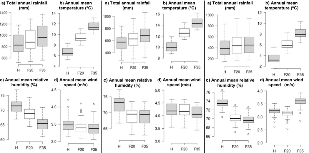
3.7 Overview of climate data

The differences in climatology between the historical and future timelines for the Ottawa, Thunder Bay and Niagara cities are presented in Figure 5, Error! Reference source not found. and Error! Reference

source not found., respectively. In the figures, boxplots of yearly totals (in case of rainfall) and yearly

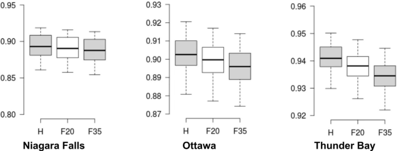
averages (in case of other variables) of temperature, relative humidity and wind speed are shown. As presented in a typical boxplot, the segment inside the rectangle shows the median of the yearly

totals/averages, the central rectangle spans the first quartile to third quartile (the 25th_{and 75}th_{percentiles),} the whiskers above and below the rectangle present the minimum and maximum values excluding the outliers, and the individual points represent the outliers. From the figures, it can be noted that in general, there will be a slight but non-significant increase in the annual rainfall in the three cities under

investigation; whereas average relative humidity will decreases over time. Average wind speed tends to decrease over time in Ottawa and Niagara Falls, and to increase in Thunder Bay at the long term.

34_{Taylor KE, Stouffer RJ, Meehl GA (2012) An Overview of CMIP5 and the experiment design. Bull. Amer. Meteor.} Soc. 93: 485-498.

(36)

a) Total annual rainfall (mm)

b) Annual mean temperature (o_C)

c) Annual mean relative humidity (%)

d) Annual mean wind

speed (m/s) c)Annual mean relative humidity (%)

d) Annual mean wind

speed (m/s) c)Annual mean relative humidity (%)

d) Annual mean wind speed (m/s)

Figure 5. Boxplot of historical (H) and future (F20 and F35) climate parameters in Ottawa. F20 & F35 respectively represent the scenarios of 2.0 and 3.5

increases in temperature.

Figure 6. Boxplot of historical (H) and future (F20 & F35) climate parameters in Niagara Falls. F20 & F35 respectively represent scenarios of 2.0 & 3.5 increases

in temperature.

Figure 7. Boxplot of historical (H) and future (F20 and F35) climate parameters in Thunder Bay. F20 & F35

respectively represent the scenarios of 2.0 and 3.5 increases in temperature.