Applying run-by-run process control to chemical-mechanical planarization and assessing insertion costs versus benefits of CMP

Applying Run-By-Run Process Control to Chemical-Mechanical Planarization and Assessing Insertion Costs Versus Benefits of CMP

by

Arthur H. Altman

M.S.E.E.(Computer Engineering) Carnegie-Mellon University, 1980

Submitted to the Alfred P. Sloan School of Management and the Department of Electrical Engineering and Computer Science

in partial fulfillment of the requirements for the Degrees of Master of Science in Management

and

Master of Science in Electrical Engineering at the

Massachusetts Institute of Technology May 12, 1995

© Massachusetts Institute of Technology (1995). All Rights Reserved.

Signature of Author / /' - L/ _1A#' <.

Certified by .

Roy E. Welsch, lfessor of Statistics and Management, Sloan School of Management

Certified by

-Duane Boning, Assistant Professor of Elect&e Engineering, Department of EECS

Accepted by

Accepted by

fA

1!1 w , I"

Jeffrey _. ks, Associate Dean, Sloan Master's and Bachelor's Programs

Frede ic R. aler, Chairman, Committee on Graduate Students

1 MASSACHIJSETTS INSTITUTE

JUN

2

0

1995

%ark8 SO

Applying Run-By-Run Process Control to Chemical-Mechanical Planarization and Assessing Insertion Costs Versus Benefits of CMP

by

Arthur H. Altman

Submitted to the Alfred P. Sloan School of Management and the Department of Electrical Engineering and Computer Science

in partial fulfillment of the requirements for the Degrees of Master of Science in Management and

Master of Science in Electrical Engineering Abstract

As semiconductor manufacturing technology progresses, it is characterized by

diminishing critical dimensions, and tighter photolithographic depth of focus windows caused by the need to resolve these shrinking features. Previously inconsequential

variations in the surface topography of thin films, combined with minimum required film thicknesses and greater numbers of film layers, are squeezing the effective window of operation of the photolithography process. Process steps that apply and extend existing semiconductor manufacturing techniques have been introduced whose sole purpose is to planarize the surface of a given thin film, to try to reclaim some of the process window. But these steps only affect relatively local regions of a film on a silicon wafer.

Chemical-Mechanical Polishing (CMP) is a method of achieving global film

planarization, using technology adopted from the precision grinding and lapping industry. By polishing an entire wafer, it is possible to achieve an unprecedented degree of thin film smoothness. However, CMP is a process technology for which the underlying physical understanding is weak, and which has many control variables. CMP process control is at an early stage of development relative to other semiconductor processing technologies. This thesis attempts to advance the state of the practice of CMP process control by applying a new algorithmic control technology, run-by-run control (RbR), to a CMP process in a production semiconductor fab. The results obtained show that RbR is a promising approach for CMP process control, however, some practical manufacturability issues remain to be addressed for RbR to successfully move out of the laboratory and onto the factory floor.

This thesis also assesses a proposal within the host manufacturing organization, Fab 4 of Digital Equipment Corporation's Digital Semiconductor Division, to introduce CMP in place of an existing planarization process. This proposal is particularly notable because it is to introduce new technology to a production CMOS process, not to a process under development. By applying a net-present-value-focused framework, the complexity of the proposal could be managed and a common reference language for engineers and

managers was established. This framework caused new issues to be addressed that were not traditionally considered, but that were vital to evaluating the proposal: the "real option" value of switching to CMP, and the cost of disruption due to introducing new technology to the factory floor. A simple model of disruption was proposed and applied based on previous academic research on multi-factor productivity.

Thesis Supervisor: Dr. Duane Boning

Title: Assistant Professor of Electrical Engineering Thesis Supervisor: Dr. Roy E. Welsch

Acknowledgments

I thank the people of Digital Equipment Corporation's Digital Semiconductor Division for hosting me during the second half of 1994. I am indebted to the engineering staff for their openness and patience in showing me the ropes, and particularly to Matt Van Hanehem, who bore the brunt of it. I thank Erik Bettez and the rest of Fab 4's

management and staff for providing helpful guidance throughout this research, and Tracy Harrison, LFM '92, for helping me stay on track.

I thank William Moyne of the MIT Microsystems Technology Lab for all his cheerful assistance with the RbR software, including installing and debugging it at DEC on yet another "almost standard" UNIX platform.

I thank Professor Marcie Tyre of the MIT Sloan School and Professor Roger Bohn of UC San Diego for their friendly advice, not to mention research materials, on the economics of new technology insertion on the factory floor.

I gratefully acknowledge the support and resources provided by the Leaders for Manufacturing Program, a partnership between MIT and thirteen major U.S. manufacturing firms, and by Texas Instruments, Inc.

Dedication

For Barb and Gabe

To the loving memories of

my mother, Beatrice Aftman

Table of Contents

CHAPTER 1: INTRODUCTION ... 8

1.1 PLANARIZATION AND CHEMICAL-MECHANICAL POLISHING ... 8

1.2 PROBLEM STATEMENT AND THESIS PLAN ... 12

CHAPTER 2: PROCESS CONTROL AND CMP ... 14

2.1 CM P PROCESS CONTROL AT DEC ... 15

2.2 LOT-LEVEL VS. WAFER-LEVEL CONTROL ... 1 8 2.3 CMP PROCESS CONTROL IMPROVEMENT CHALLENGES ... 20

2.4 RUN BY RUN PROCESS CONTROL... ... 21

2.5 CHOOSING THE CONTROLLED RESPONSE ... 23

2.6 CHOOSING THE CONTROL VARIABLES...26

CHAPTER 3: DOE APPROACH AND RESULTS ... 29

3.1 STATISTICAL DOE... ... 29

3.2 EXPERIMENT #1 ... ... 33

3.3 E X PERIM EN T #2 ... 37

3.4 BACK END CM P EXPERIM ENT #1...39

3.5 B ACK END E XPERIM ENT #2 ... 44

CHAPTER 4: RBR EXPERIMENTAL APPROACH & RESULTS ... 46

4.1 RBR TEST ... ... ... 49

4.2 RBR TEST RESULTS ... 52

CHAPTER 5: ECONOMICS OF CMP AS A REPLACEMENT FOR AN EXISTING PLANARIZATION PROCESS ... 58

5.1 A NALYSIS A PPRO ACH ... 60

5.2 DECISION FRAMEWORK ... 61 5.2.1 C heap er?... ... 6 1 5 .2 .2 F a ster? ... 62 5.2.3 B etter? ... ... 64 5.2.3.1 C ore C om petency ... ... 64 5 .2 .3 .2 Y ield ... ... 6 5 E conom ic B enefits ... ... ... 66 Y ield M odeling ... ... ... 68 5.2.3.3 D isruption ... ... 69

5.2.3.4 Options and Contingencies ... ... 76

5.3 SUMMARY... 80

CHAPTER 6: CONCLUSIONS ... 81

6.1 DESIGN FOR RUN-BY-RUN CONTROL ... ... 81

6.2 MANUFACTURABILITY OF RBR CONTROL ... ... 83

6.3 TECHNOLOGY INSERTION STRATEGY ... ... ... ... 85

REFEREN CES ... 87

A PPEN D IX ... 90

DATA AND REGRESSION RESULTS OF EXPERIMENT #1 ... 90

DATA AND REGRESSION RESULTS OF EXPERIMENT #2 ... 129

DATA AND REGRESSION RESULTS OF BACK END EXPERIMENT #1 ... ... 149

Chapter 1: Introduction

1.1

Planarization and Chemical-Mechanical Polishing

The march of silicon-based integrated circuit technology to deliver ever more functional sophistication and performance at ever decreasing prices has continued unabated for over thirty years. The primary driver of this cost/performance

juggernaut has been that each new technology generation has enabled smaller devices, more densely packed and connected together on a silicon die, than the generation that preceded it.

This in turn has imposed increasingly more challenging technical and business goals upon semiconductor manufacturers. Semiconductor manufacturing consists of a

series of photolithographic steps, in which successive layers of metals, dielectrics, and other materials are deposited and patterned in such a way as to form electronic devices connected in a functioning circuit. The need to shrink device sizes and space them more tightly has squeezed the required minimum feature size to be

photolithographically discerned down to sub-micron levels. The need to connect exponentially growing numbers of devices together to realize such complex products

as microprocessors, along with the challenges of building working, reliable transistors in shrinking dimensions, have increased the number of layers and the

2 complexity of each layer of a semiconductor product.

The optics of reducing minimum feature size (also known as critical dimension, or CD) require an increasing numerical aperture (NA) in the focusing lens of the photolithographic stepper, so that it can gather enough light to give the necessary resolution to the image to be printed on the silicon wafer. However, that resolution will only be achieved within a certain depth of focus above the wafer surface. Thus horizontal CD shrinkage affects vertical focus latitude. Specifically, depth of focus is inversely proportional to NA squared, whereas CD is inversely proportional to NA.

So, for example, doubling NA to cut CD in half cuts the corresponding vertical focus range by a factor of four for a given exposure wavelength of light.

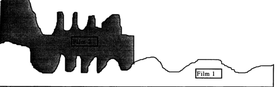
The surface topography of each layer of an integrated circuit reflects the topography of the layers beneath it. Topography accumulates from layer to layer, as patterning produces regions where certain layers are absent, abutted by taller regions having fewer omitted layers. The increasing number of layers in modem integrated circuits compounds this effect, to the point that the vertical topography of a complex integrated circuit could be quite severe (see Figure 1.) That is to say, severe enough to give the photolithography step insufficient process window to accommodate its rapidly diminishing depth of focus. Also, severe enough to cause many other defect modes, such as poor step coverage of deposited films and residual material after dry etching.3 _{The negative impacts of topography are expected to be most severe at the}

highest film layers, namely those of the metal lines that interconnect the transistors; as complex logic demands three, four, or more metal wiring levels, this becomes critical.

Film 2 Selectively Deposited Over Film 1

Figure 1: VLSI Processing Topography

Therefore, there is a clear need to not only deposit and pattern films, but to planarize them, that is, to reduce the topography across the surface of a die, if not the entire wafer. Planarization techniques such as plasma etchback4 _{have been developed to}

a given surface layer to try to cover over its topography, and subsequent nonselective etching steps to "etch back" the combined layers to some acceptable overall

thickness. This can also be supplemented by gap filling between closely-spaced structures. All of these techniques build upon existing semiconductor unit processes such as dry etching, although the added films may include specially designed materials such as spin-on glass.5

There are, of course, degrees of planarization of topography. The above techniques are successful at smoothing and local flattening of steps, what is referred to as

"local" planarization. (Referring back to Figure 1, these techniques would have a smaller impact on Film 2 topography the wider the spacing between adjacent Film 2 peaks.) None of these techniques achieves "global" planarization, which is the absence of topography over the surface of a deposited film, across the entire wafer. 6,7 At four or more layers of metal, with technology CDs of 0.5 micron and below, the photolithographic depth of focus process window provided by the above techniques is relatively narrow. Fortunately, it is now possible to ameliorate this situation by using new photolithographic I-line steppers featuring variable NA.8 These steppers can be set to trade off resolution for depth of focus at any layer; this is especially useful for the higher metal levels where wider lines than those needed to make transistors are acceptable.

But this approach does nothing to reduce the defect modalities caused by topographic irregularity, and in some cases it may be prohibitively expensive to upgrade to the newer stepper technology. The consensus seems to be that to enable state-of-the-art and future IC fabrication, global planarization of multiple deposited layers is required.9 To achieve this, a different approach to planarization technology has been developed recently, Chemical-Mechanical Polishing, or CMP. CMP applies precision industrial polishing technology to sub-micron VLSI requirements. By polishing the entire wafer it is possible to achieve global planarization, and with fewer individual steps than deposition/etchback processes require.-o

The principle of operation of CMP is to press the wafer surface to be polished against a rotating polish pad; a slurry (e.g., consisting of silica particles in water and KOH, in the case of polishing silicon dioxide) is applied to the pad as it rotates. A

combination of mechanical abrasion (due to the pad and slurry particles) and

chemical etch (due to slurry chemistry) causes material to be removed from the wafer surface. Because areas that protrude erode more efficiently than areas that are

recessed, this process planarizes the wafer surface.

Wafer Carrier

Slurr

Platen

A diagram of a CMP tool, adapted from " is shown in Figure 2. The wafer is held on a rotating carrier backed by a special carrier film as it is polished. It is possible to vary the wafer and pad rotational rates, pad temperature, the downforce applied by the carrier, and many other parameters to achieve a nominal polishing rate and rate variation across the wafer. The process consumables, namely the slurry, polish pad, and carrier film, all affect process behavior and manufacturability, i.e., the ability to maintain constant process behavior over time.12 _{For instance, as a wafer is polished,}

polish debris accumulates on the pad, reducing mean polish rate across the wafer. Pad conditioning, abrading the pad to expose fresh pad material to the polish process, is used to counter this process degradation.13_{CMP planarization is also sensitive to}

pattern density, so that equivalent layers (e.g., first inter-level dielectric) on different VLSI chips can experience different polish rates under the same CMP "recipe."1 4

Despite the heritage of CMP in decades of precision industrial polishing, the detailed physical behavior of the polishing mechanism is still not fully understood.15 _Progress

in CMP in the VLSI manufacturing setting has meanwhile been driven by empirical knowledge acquired by experimentation and cumulative experience. As a rough

dT

model, Preston's equation, - = KPV, is often used, especially when polishing dt

oxide. It says that the rate of oxide removal increases with applied pressure (P) between the wafer and pad, and with increasing relative velocity (V) of the wafer with respect to the pad. K is a constant of proportionality that encapsulates other process variables such as pad temperature. Preston's equation has been shown to track experimental results in the literature,16 _{but it falls short of being a complete} predictive model of CMP process behavior. For example, it does not model polish rate variability across the wafer.

1.2 Problem Statement and Thesis Plan

In CMP, then, we have a process technology for which underlying physical

understanding is weak, and which has many identifiable (and perhaps a few more as-yet-unknown) control variables. Not surprisingly, then, CMP process control is at an early stage of development relative to other semiconductor processing technologies. This thesis attempts to advance the state of the practice of CMP process control by applying a new algorithmic control technology, run-by-run control (RbR), to a CMP process in a production semiconductor fab.

We have already noted the need for planarity throughout the integrated circuit

fabrication process, so it should not be surprising to find CMP applied at many stages of the process. However, CMP may not always be the best choice everywhere in the manufacturing sequence. This thesis also assesses a proposal within the host

Semiconductor Division, to introduce CMP in place of an existing planarization process. This proposal is particularly notable because it is to be a "retrofit," introducing new technology to a production process, not a process under development.

The next chapter describes CMP process control at DEC, and introduces the run-by-run control method. Chapter 3 describes the experimental approach taken to obtain CMP process models for use by the RbR controller, and the results of those

experiments. The next chapter describes the method and results of testing RbR in controlling a CMP process. Chapter 5 discusses the application of a framework for assessing the CMP retrofit proposal, how such effects as performance disruption and yield improvement were modeled, and how the strategic value of CMP could be put into dollar terms. The thesis concludes with lessons learned and suggestions for future work.

Chapter 2: Process Control and CMP

Manufacturing processes transform a set of material and other inputs into a desired combination of material properties and geometry, i.e., the product. The resulting product characteristics almost always exhibit some deviation, however slight, from the target result, and so tolerances must be established. Tolerances distinguish products that are unacceptably off target from those having negligible variations, and also separate

correctly functioning but "lower-performance" products from "higher-performance" ones. Manufacturing process control attempts to minimize products' deviations from their target geometry and properties, to thereby maximize the number of "within-tolerance" and/or "maximum performing" products made by a given process.

Before CMP After CMP

Figure 3: CMP Planarization

As shown in Figure 3, for CMP the task is to transform a thin film having arbitrary topography across a wafer into a flat film. The resulting film will possess a nominal thickness that is a function of its pre-polish thickness, the underlying topography of previously deposited films, and the planarizing performance of the CMP machine. Typically, a pattern of point locations across the wafer is selected for measurement, and

these points will be at the same location within a die*. (Thin film measurement systems such as the Prometrix 650 and 750 used in this research support such wafer pattern specification.) Therefore each pattern of points will describe a particular (replicated) vertical section of the film. It should be noted that the underlying topography is only captured by tracking multiple patterns of distinct point locations.

Some material properties of the thin film may be altered by the polishing process. For example, foreign particles previously embedded in the film may be removed by polishing, or the dielectric properties of a polished oxide may be altered at the surface17_{. These}

changes constitute responses to be characterized and controlled; understanding them is important to integrating CMP into the overall CMOS manufacturing process.

However, important as they may be, polishing-induced material property changes are nonetheless side-effects (good or bad) of CMP. The primary motivation for polishing is to alter film geometry. This thesis focuses on the geometry process response and how to improve its quality. To set the stage, it is necessary to first understand how polished film geometry was being controlled in Fab 4 of Digital Semiconductor at the beginning of the author's internship there, and the results that were typically obtained.

2.1 CMP Process Control at DEC

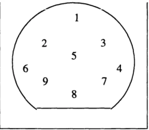
Digital Semiconductor, a division of Digital Equipment Corporation, uses CMP in its 0.5 micron CMOS manufacturing facility in Hudson, MA. In its current application, CMP polishes a deposited oxide film down, breaking through an underlying silicon nitride layer, and continuing for a pre-calculated amount of time, with the goal that a specified mean thickness for the nitride film is achieved. A nine-point pattern across the wafer is

t used similar to that shown in Figure 4 to obtain spatial information across the wafert

Each "point" is chosen by the process engineer such that the area covered by the point's spot size is relatively uniform; it doesn't span a pattern of features.

"A note on wafer geometry: wafers are sliced from a cylinder of silicon, and a tip of the resulting circular wafer is cut to

Figure 4: Approximate Film Thickness Measurement Pattern

Each point is at the same location within a VLSI chip (die). For that point or vertical section, process engineers have determined the target silicon nitride thickness to be achieved. The key feature of the nine-point pattern is that it provides, roughly, a center point surrounded by a 4-point middle ring and 4-point outer ring. The points in the outer ring are at angular offsets with respect to the middle ring, to increase the spatial

information obtained. (Due to the geometry of placing die within a wafer, any collinearity of three points in the pattern is a chance occurrence.) In choosing the number of points, engineers traded measurement time and cost against ability to characterize film thickness across the entire wafer.

In this context there are (at least) two ways to characterize the film geometry after polishing:

* What is the average film thickness across a wafer and how does it vary? * What is the range of film thicknesses across a wafer and how does it vary?

These are statistical measures that summarize the raw data obtained from the 9-point film thickness measurements. The criterion for using them is that they can be used to capture the film thickness variability within a wafer, from wafer to wafer, and from lot to lot. These are also the measures used within DEC, and so are used herein for consistency and convenience. (Qualitatively, the "average" refers to the arithmetic mean of a group of measurements, while the "range" is the difference between the maximum and the minimum values within the group. These measures will be formally laid out later.)

The same nine-point post-polish data measurements, combined with corresponding pre-polish data measurements, can be used to determine the pre-polish rate of the CMP machine, and permit its variability to be evaluated and tracked in the same way as ending film thickness. In a manufacturing setting such data may be available as part of tracking the process that precedes CMP, otherwise it will have to be obtained as part of the CMP operation in the fab.

Having identified the process responses of interest, DEC process engineers used statistical design of experiments (DOE) and response surface techniques8 to arrive at settings for carrier and pad rotational speed, choice of polishing pad material, and other CMP machine input parameters that would give the "best" CMP process response for polish rate. All settings were to be left unaltered by machine operators on the

manufacturing line. For each lot of wafers, the time spent polishing would be calculated by the operators based on the latest machine polish rate information.

This approach was motivated by the significant drift in polish rate exhibited by CMP machines. By significant drift, I mean that the overall average polish rate, as well as the variability of the polish rate across the wafer, consistently deteriorated as the cumulative number of wafers polished rose, and could reach one or more lower control limits within a few hundred wafers. Why does this occur? Polish pads and other consumables have finite lifetimes, and their key polishing properties degrade with cumulative wafers

polished, even with pad conditioning. ("Aggressive" - frequent, lengthy, and/or maximally abrasive - pad conditioning reduces the effect, but also reduces pad life, increasing materials costs and time-consuming pad replacements.) The good news is that since this drift makes the process unstable from a "Deming" perspective,19 it should be possible to compensate for errors without over-controlling, i.e., without making the situation even worse.

Another reason to focus on machine polish rate is the variability of the incoming oxide and nitride film thicknesses. For instance, a wafer that receives a thicker oxide deposition will require a longer polish time to achieve the target thickness. Under these

circumstances, assuming an unchanging polish rate and pre-polish film thickness and then selecting a fixed polish time for the CMP process should not be expected to give a high Cpk result*.

2.2 Lot-Level vs. Wafer-Level Control

The ideal way to control the polishing process would be to measure film thickness in detail across the wafer while it is being polished, and to use real-time feedback control to adjust the polish time and other machine input parameters, for each wafer polished, to optimize resulting film variability and mean thickness. The sensing technology required is not widely available, however,2 0 _{and was not provided by the CMP equipment vendor.}

(Such a real-time, wafer-level approach is being explored elsewhere, but on other processes.21 )

What is readily possible is to measure films before and after polishing. The DEC process engineering staff therefore developed a lot-level, manual closed-loop control system for

CMP. This system requires that a number of unpatterned, non-product "monitor" wafers be polished, and that a number of thickness measurements be made, for every product lot.

*Cpk, also known as the process capability ratio, is a statistical measure of the ability of the process to produce within-spec results.

The CMP machine operator plugs the information thus gained into some simple formulas that have been developed from experience. The operator uses the results to set the

polishing time for each lot, roughly compensating for changing grand mean polish rates and grand mean incoming thicknesses. Starting with this time setting, a pilot wafer from each lot is first polished and measured, and the polish time for the rest of the lot is

adjusted if the results so indicate. The polish time is thus fixed for all but one wafer in the same lot.

This approach keeps the average post-polish thickness for the wafers in a lot close to specified limits, even as the polish rate degrades, by adjusting the polish time. Eventually, the polish rate will degrade so far that the cycle time of the CMP machine is judged to be unacceptably low; in this case consumable items may be swapped and/or other

adjustments may be performed to "reset" the machine state to a higher polish rate. The need to process monitor wafers adds to the fab's operating costs, since monitors do not become products.

Statistical process control techniques are used to deal with thickness variability caused either by incoming thickness variation or by polish rate variation. The operator waits for certain polish rate variability measures, such as the percent difference in center-to-edge polish rate, to exceed specified limits, and then acts to bring those measures back in spec, again by replacing consumable items and so on. These measures being out of spec do not correspond to out of spec polished product, but signal that it is likely that product will go out of spec soon, possibly on the next run, unless corrective action is taken. This is a practical approach for avoiding producing scrap, but unlike the case of decaying mean polish rate, the operator has no means to compensate for decaying variability as it occurs, because all other machine settings are held constant.

Since DEC first developed and applied this CMP process control approach, one

commercial vendor has begun to market a CMP endpoint detection tool. This is a system that promises to signal in real-time that the target thickness for a polished layer has been

reached. With this technology, polish times could be automatically adjusted for each wafer to compensate for differences in mean starting thicknesses and polish rates. Film thickness uniformity control would remain unaddressed, however.

This endpoint detector, the Luxtron 2350, tries to capitalize on the observation that, as material A is polished down to material B, the polisher can signal the difference in coefficient of friction between the two materials. This is because the polisher adjusts its wafer carrier motor controller current to compensate for the friction change and maintain a steady wafer rotational rate. By tapping onto the carrier motor controller signal and processing it, the Luxtron 2350 tries to provide a signal that can be reliably used to detect endpoint. This approach was claimed by Luxtron to work well for CMP applications such as DEC's. However, for the case of interlevel dielectric polishing, where the oxide

between two metal layers is to be polished down to a target thickness, this approach does not work because no material interface is crossed.

Over the course of 4 weeks at DEC I tested the Luxtron 2350, but found that the signal it provided did not distinguish between oxide and nitride layers at all, even when

unpatterned oxide-over-nitride layers were polished. (On actual product, due to

patterning, less than half the surface will have any nitride under the oxide, so polishing blanket wafers is a best-case test scenario for the 2350.) The reason was that the 2350 was designed to work with newer polisher models than those installed at DEC; the new

models have different, higher-quality motors and motor controllers. We appeared to be in a "garbage in, garbage out" situation, with the polisher motor was providing an

unacceptably poor input signal to the 2350.

2.3 CMP Process Control Improvement Challenges

The DEC approach works well in the factory, but the question is, can we do better, particularly with respect to three issues:

* Rather than passively watch polished films become steadily less and less uniform until the machine is reset, can we actively compensate for machine "wear"? * Can we polish fewer or zero non-product wafers?

* Can we automate parameter compensation to reduce the chance for operator errors and permit more complex, optimized compensation calculations?

Of course, this should be accomplished while achieving as good or better mean thickness results than are already achieved by manual closed-loop control.

2.4 Run by Run Process Control

Over the last few years at MIT, as part of ongoing research into semiconductor manufacturing process control,2 2 _{an on-line technique for process control has been}

developed, called "run by run" (RbR) process control23_{.The RbR controller modifies the}

process recipe on each lot or "run," based on data collected in the previous run. So-called "gradual mode" RbR controls the process to target in the presence of drift. The key assumptions of gradual mode RbR control are that:

1. The process exhibits systematic drift in one or more responses;

2. The process has at least one control variable that can be conveniently adjusted between runs;

3. Each drifting response (y) to be controlled can be modeled (or be transformed to be modeled) as a first-order function of control variables (xi), i.e., y = a + Xbixi

4. There are no statistically significant interactions amongst the control variables (i.e., no xixj cross-terms);

5. Process drift can be modeled more or less as a change to the intercept a, i.e., the

process's sensitivity to adjustments to xi is fairly stable over time.

In the rest of this thesis, I will use the adjective "first-order" as short hand for the mathematical model described by points 3 and 4 above. Note that while the model can describe a simple quadratic or other non-linear relationship between the response and a given control variable (by suitable transformation of the control variable), it does not admit more complex relationships, such as a linear term plus a quadratic term. (While one

could transform the non-linear terms, e.g., renaming 'X2 ' _{to be 'w', the controller would}

in practice try to adjust x and w separately; the current RbR software treats each control parameter as independently adjustable. William Moyne lays out the algorithmic details and limitations in his thesis24_.)

Under these assumptions, the RbR controller provides two algorithms to control the process to target. One is based on an exponentially weighted moving average (EWMA) algorithm, while the other uses the predictor-corrector (PCC) algorithm.25 Both work to conservatively adjust the process model by updating the constant term a to reflect current process behavior. The EWMA algorithm locates a "new model target contour" that represents the drifting process, and selects a setting for xi on the contour that minimizes the distance from the previous setting. The stability and robustness of the EWMA-based controller were studied2 6 _{and found to perform well over a wide range of drift behaviors.}

This approach has been tested in a few semiconductor processes, such as plasma etching,27'28 in laboratory settings. Essentially, the EWMA algorithm implements a simple integral controller.

The PCC algorithm is a two-level EWMA; the practical effect is that it provides a forecasting mechanism that can quickly and effectively react to drifts and to changes in drift rate and direction. It also suggests no changes when it sees only random fluctuations in a process response. Both algorithms are parameterized to permit the amount of history and/or the aggressiveness of the forecasting to be adjusted.

Having updated its internal model of the process using EWMA or PCC, the RbR controller then sets the control variables for the next run by solving the set of

simultaneous equations that describe the responses, such that the vector of responses will be as close as possible - in a least squares sense - to the target vector of responses.

Reflecting upon the CMP process control challenges described earlier, RbR control appears to be a promising approach. It need not collect data from monitor wafers; it is

automated; it requires no new sensing, measurement, or control hardware for the CMP machine; and most importantly, it holds out the practical possibility of film uniformity drift compensation. Another attraction is that the algorithms have been implemented

29

within a UNIX-based software environment designed for portability and ease of use29

and can be obtained free of charge to U.S. industry.

However, the effectiveness of RbR is clearly limited by the fidelity of the first-order response model to actual process behavior. There is no research demonstrating just how much process variability must be explained by this model for RbR to work. A research group at San Jose State University and National Semiconductor is applying RbR to CMP30_{, developing an optimized laboratory process and sophisticated behavior models,}

such as for "pad rebounding." The SJSU group has reported success using a primitive process model but has not provided details in the literature. As of this writing, no other work has been published on applying RbR control to CMP, although an R&D project by SEMATECH, University of Michigan, and MIT is underway.

2.5 Choosing the controlled response

As has been noted by other researchers of model-based manufacturing process control,31 it is not necessarily the case that the best response for monitoring is also the best response for controlling a process. In the particular case of RbR, statistical summaries designed to give the maximum insight into process behavior will not necessarily have the first-order functional behavior described above, nor should they be required to do so. Conversely, it may or may not be particularly helpful to equipment operators, technicians, and engineers to chart a measure chosen only for its compatability with the premises of RbR.

A useful set of monitoring statistics was already being charted for the CMP process at DEC, as mentioned earlier. These summaries were obtained from raw thickness data measured at each of nine points; four wafers from each lot are sampled to collect this information. The measures for each lot were: the grand mean film thickness (TT) and the range of mean film thicknesses (RT); the mean film thickness range across a wafer (TR) and the range of film thickness ranges across a wafer (RR); the grand mean polish rate

(P); and the polish rate "nonuniformity." The first four measures concern themselves with the product result, while the last two focus on process behavior.

To define each of these measures, let Xijk be the film thickness at the ithi site of the jh wafer of the kh lot polished, then:

94 1: 1:xijk k i=1 j=1 36

RTk=

9

9

Xilk)

(

-= M

IN

(MAx(xj

, X

jk

,...,

X

k

)

-

MIN(X

jk,

X

k,...,

X

jk))

4

(MAX

(XkX21k,...X91k)-MIN(XIkX21k,...,Xj

)

,

RR MAX

RR, = MAX

(MAX(x,

)-

(MAX

)-

MIN(X]

k

IN

MIN(XI

))

(MAX

)-

(MAX

)-

Let Yijk be the initial film thickness, and Tk be the polish time for the lot, then the mean polish rate is:

_ -(2 Xl, Pk =

The polish rate nonuniformity for a wafer is measured by taking the polish rate for the site closest to the center of the wafer, subtracting from it the average of the polish rate for the points on the 4-point outer ring, and dividing by twice the mean polish rate for all nine points. This gives a nonuniformity measure from the center to the edge that ranges between ± 100%. The polish rate nonuniformity for a lot is defined as the mean of the nonuniformities for the four sampled wafers in each lot.

Engineering intuition about the polish process indicated that while the means might have first-order response models, the ranges and nonuniformities were unlikely to exhibit such simple relationships to CMP process parameters. Specifically, any measure of film thickness variability would summarize the spatial variation of the polish process, which was expected to be complex. (For example, the polish rate near the wafer flat is often different from the rest of the wafer.) It also seemed risky to try to predict a priori the "best" statistic for controlling the variability of CMP; research on spatial uniformity control by Guo3 2 _{suggests that using a single spatial uniformity metric to direct on-line}

process control may be a weaker approach than "unbundling" the metric into unsummarized spatial responses.

So rather than use DEC's CMP process charting and control measures, I decided to use the nine-point data from each sampled wafer directly, that is, to have the RbR control a nine-element response vector Y corresponding to the final polished film thicknesses at the nine measurement sites. I would specify that each site be polished to the same target thickness. In solving the resulting simultaneous equation for the best least-squares error over the nine sites, the RbR algorithm would obtain one type of "optimum" balance of mean film thickness and film thickness variation within a wafer and within a lot. (The controller would in fact treat mean thickness and thickness variation with equal

modeling individual sites on a wafer: the expectation was that the response at any one site would be well-modeled by a first-order equation.

Before we leave the question of which response to control, consider the possibility of putting the polish rate at each site under RbR control instead of the final film thickness. This would be consistent with the common process control focus on machine behavior rather than on product characteristics, and harkens back to Preston's equation. However, it suffers from two weaknesses that cause me to stick with film thickness, at least for now:

* "Polish rate" is not directly measured, but is itself a summary measure, and so is potentially filtering information from the controller (e.g., initial film thickness variation);

* Polish rate would still need to be converted from "response" to "control parameter" form to enable the RbR controller to determine a lot's polish time, which poses an added complication compared to using final film thickness.

2.6

Choosing the control variables

If Y is the target thickness vector, what are the components of X? To begin, the RbR controller could adjust polish time for a given lot. But one input parameter would not be sufficient to control both the mean and the variation in film thickness. But which of the other CMP process control variables should be chosen? Here, a constraint was imposed by the manufacturing, as opposed to laboratory, setting of this work. To obtain

permission eventually to try out RbR on the manufacturing line, the controller would have to avoid modifying the existing, production-qualified CMP process recipe.

Otherwise all chips made while RbR was being tested would be automatically assigned "nonconforming" status, which would have made the cost of the experiment to the fab unacceptably high. So only input parameters that were unused by the process recipe were viable candidates to be RbR control variables, in addition to polish time.

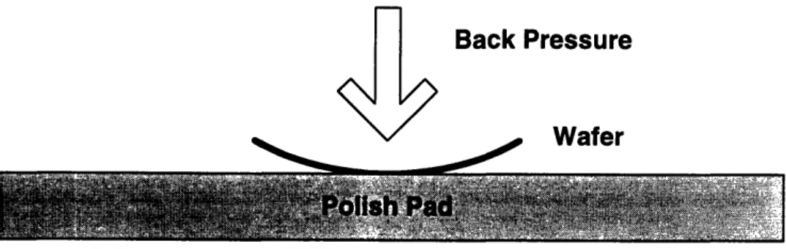
Fortunately there was an unused input parameter that could be easily and accurately set by the operator from one lot to the next: back pressure. As illustrated in Figure 5, the CMP wafer carrier can apply air pressure to the back of the wafer as it is being polished, which "bows" the shape of the wafer against the polish pad. In this way, polishing rate

variability can be altered without changing any other input parameter. Specifically, the center of the wafer is expected to polish faster while the outer edge is expected to polish

slower than the grand mean polishing rate. While this clearly is not a fully general film thickness uniformity control variable, it does give the RbR algorithm something to work with within the stated operating constraints, and it is not obvious a priori that full generality is needed. (A "fully general" variable would permit thickness adjustment in any direction for any of the 9 points.)

Back Pressure

Wafer

Figure 5: Back Pressure Effect

The lot-to-lot response to be controlled was therefore expected to take the form:

F = A, + BInit, +CT +DP +EPJ~, +GP 2 _+HT 2

for each point i and each lot j. (To get a lot's response, a number of wafers from each lot are sampled.) Here, F is the final film thickness, Init is the initial oxide film thickness, T is the lot polish time, and P is the back pressure; the same T and P are applied to every wafer in a lot. B is expected to be a positive coefficient, C a negative one, while D and E should be negative in the center and positive at the wafer edge. This equational form only makes the claim that higher-than-quadratic-order terms are not expected; the exact form of the response will be that which best explains the experimental data. The actual, empirically determined response might or might not include the P term, the PT

interaction, or higher-order terms. How close we could come to the specific first-order RbR model would remain to be seen.

The back pressure terms in the above equation deserve some comment. From a physical perspective, back pressure could possibly act in two ways. It could combine with polish time to remove more or less material, or it could act as an offset to the amount of material removed, independent of polish time. The former action corresponds to basic intuition about the continuous effect of applied pressure over time. The latter action reflects the case where the magnitude of back pressure relative to the magnitude of the polish arm downforce applied by the CMP machine (the P in Preston's equation) is particularly small. Then, if there is a back pressure effect at all, it is likely to be a result of the

geometric bending of the wafer rather than the (negligible) change in effective downforce. This could yield an effect that is decoupled from polish time and is more akin to the other geometric effect, changing initial film thickness.

'Init' is a covariate, a parameter that affects the outcome but over which the CMP process has no control. It is not the combined nitride and oxide thicknesses, but just the thickness of the oxide over the nitride film. This is a consequence of the following: (1) the nitride film thickness was tightly controlled across the wafer, and so could safely be treated as a constant without jeopardizing the RbR experiment, and (2) to have required the nitride film thickness be available for every point, for all wafers to be sampled (if not 100% of the wafers) would have entailed a significantly more costly level of tracking than what

was presently used by the fab, and at a time when the fab was looking for ways to reduce its data collection overhead. The oxide thickness at each point for each wafer could be easily obtained before a polish operation, and without imposing extraordinary costs on the fab.

The next chapter discusses the statistical design of experiments and the resulting behavioral models to be used by the RbR controller.

Chapter 3: DOE Approach and Results

This chapter begins by describing the statistical design of experiments (DOE) approach I used to characterize the Fj response surface. The remainder of the chapter discusses the results of linear regressions on the experimentally obtained data. The regression

coefficients are to provide behavioral models for use by the RbR controller. The reader should note that, to protect Digital Equipment Corporation proprietary data, all reported time units, be they minutes or seconds, have been multiplied by "fudge factors" to conceal actual CMP polish rates and times.

3.1 Statistical DOE

I designed an experiment to characterize the final film thickness at each of 9 wafer sites as a function of initial thickness, polish time and back pressure. In designing the

experiment, I made the following assumptions:

* A number of wafers could be polished one after another in the same cassette, under different settings of polish time and back pressure.

* The number of wafers polished (experimental runs) would be small enough that CMP process drift would not affect the results. If this assumption were wrong, drift could be accounted for by an analysis of covariance, using wafer number as the covariate. * The multiple regression results would probably show at least first-order behavior, and

interactions between polish time and back pressure were quite possible. * Initial thickness would be a measurable parameter provided by previous

manufacturing steps, but not a controlled experimental design factor. Therefore it would be a covariate, a variable that affects the (regression) results but is not controllable.

If there were interactions amongst variables, and/or curvature in the response, the actual coefficients for those terms would be of interest , so the experiment should be designed to provide such information. The experimental design need not make an a priori choice about which terms will be (statistically) significant: it only need be general enough to capture the highest-order terms we expect to encounter. In particular, the design must be powerful enough to capture the effect of back pressure alone and its interaction with polish time, as was discussed in the previous chapter.

The assumption that the initial oxide film thickness is a covariate for the purposes of this experiment is assailable. While it is true that in actual production the CMP process can only accept in coming thickness as an input, having been determined earlier in the manufacturing sequence, the necessarily non-production nature of the experiment could have been leveraged here. That is, I could have added special instructions to the

experimental lots, requesting that they be specially processed to provide certain oxide thicknesses. In this way, I could have provided an experiment which more fully captured the response surface, whereas the range provided by the covariate approach was limited by the variability of the oxide film deposition process. However, as will be discussed, there were already significant challenges in mounting this experiment in a production setting, and I judged the incremental cost of making this improvement to be quite high in this context.

Another constraint was that the number of wafers available for experimentation was going to be limited to two lots (50 wafers total), including RbR experiments. This was a consequence of the high cost of materials and processing, and of the low priority and ever-shrinking permitted number of non-product wafers in the manufacturing line. In fact, the two lots would be available weeks apart, so it was important to get started with the first lot when it arrived.

*Not because the RbR controller can use them, but because they could be used by the simulation package supplied in the MIT software to model the "actual" equipment being controlled.

Also, the time available on CMP tools to run experiments would be very limited. For the testing of RbR, which would require many continuous hours of processing, time on the CMP machines would have to be pre-negotiated with the production group, but that group would not hesitate to "bump" me if actual conditions in the fab warranted it. (At first, I could straightforwardly schedule time on weekends, but later the fab moved to production 7 days a week, which made it less clear when and how such experimental time slots might become available.)*

For the response surface experiments of this chapter, I decided to run as few wafers as possible, and to "jump in" at some point most convenient to the operators and as close as possible to the time when I expected to able to try out RbR, since the machine state I would capture with the response surface experiments would be changing as the operators polished product lots in the interim.

I decided to run a single experiment to characterize the process as a function of back pressure and polish time. I needed to account for more than just the presence or absence of curvature, so augmenting a 22 _{design with center points alone would not have imparted}

enough information. I chose a central composite design33 _{(CCD) approach to capture the}

quadratic response surface within the practical ranges of time and pressure.

However, the CCD needed to be both rotatable and orthogonally blockable34_{. Rotatability}

is needed for equal estimation accuracy in all directions, and is a common requirement. Orthogonal blocking would have let the experiment be run a few wafers at a time over

*This is a good illustration of issues that arise trying to perform experiments in manufacturing settings. I sat down with the production supervisor and made the case that it was worth his while to sacrifice some productive time on the

machine to permit me to run my experiments. He couldn't have cared less about the thesis research, of course, the payoff to him was the possibility of saving operator time and improving quality down the road. Even at that, this person was much more accomodating than the norm, which I attribute to his background in a pilot fab; in most

manufacturing settings I would have required substantially more political muscle than I needed here. In the end for the RbR test, I was fortunate that an operator was suddenly out on a special project, leaving a CMP machine unexpectedly free for use for half of Monday and half of Tuesday over a few weeks.

separate time periods, in the event that machine access for experiments was extremely tight.

But it turns out that a CCD is difficult to block while remaining 100% rotatable. Note that a CCD requires 5 settings for each input parameter: very low (-a), low (-1), medium (0), high (1), and very high (a). For a two-input experiment such as this, the CCD will specify some combination of center points (0,0), corner points (±I1,±1), and star points (•a,0) and (0,±a). Looking at the number of corner, start, and center points in the design, it turns out

Scorner - (star + center,)

-that a =

(corner)

center2-givs

K2.-(corner

determines a for a two-block design. In general, it is difficult to exactly satisfy both equations. Software developed at DEC35 suggested a = 1.2 to give a "highly" rotatable design supportive of orthogonal blocking:

Center Point (0,0), plus 5 replications

Corner Points -1, -1 -1, , -1 1,

Star Points -1.2,0 1.2,0 0, -1.2 0,1.2

With 4 corner points, 4 star points, and 6 center points, this gave 14 runs to be performed in randomized order, leaving 36 wafers for future experiments.

For the mapping of normalized experimental settings to actual polish time and back pressure settings, I relied on advice from DEC process engineers based on their experience with the existing CMP process. I chose allowable polish time ranges of between 80 and 140 seconds (1 second settable precision). Then, for back pressure, since too high a setting could push the wafer out of its carrier, I chose 3 psi as an upper limit, which was well below the maximum for the tool. The lower limit for back pressure was zero psi, with 0.1 psi settable precision throughout the range.

At this point, the reader should note another limiting impact of the covariate assumption for initial thickness: it will not be entirely sufficient to use regression results alone as validation that there is no interaction between initial thickness and polish time or back pressure. Again, this is because the experimental design doesn't encompass initial

thickness as a control variable. However, in theory, we could fall back on simpler graphical analysis methods of the experimental results: plot the final thickness against initial thickness, with different fixed values of polish time and back pressure, and look for intersecting versus parallel lines; parallelism would tend to validate the absence of

interactions, while intersections would indicate interactions. But this would require that at least two (time, pressure) pairs be replicated in the design, so that at least two lines could be drawn. Since only the center is replicated, there is insufficient data to do this. Since at the time this experiment was designed such interaction seemed unlikely, this became a tradeoff between thoroughness and cost: the expected value of the data was judged to be less than the cost of obtaining it*, since appropriate replicates could certainly have been added to the experiment.

3.2 Experiment #1

After obtaining a suggested randomized ordering from a statistical software package, and mapping the x values onto the parameter ranges, I arrived at the experimental design shown in Table 1. The next step was to obtain the experimental material. In this manufacturing setting, this consisted of:

1. Being scheduled to use one of the lots assigned to engineering experimentation-available slots were few and dwindling as volume production increased in the fab; 2. Specifying the "route" the lot would take through the production sequence until it

reached the CMP step, including any pre-experiment measurements I might request to be made by the operators or "holds" to be personally made by me.

SIn fact, with production pressures being what they were, it never seemed to me that this was a true option, and I never tried to get permission to do this from the production supervisor.

Run # Wafer # Polish Time Back Pressure Point 1 12 110 1.5 Center 2 2 85 0.3 Corner 3 11 110 3.0 Star 4 10 110 1.5 Center 5 15 135 2.8 Corner 6 5 110 1.5 Center 7 22 85 2.8 Corner 8 1 110 1.5 Center 9 21 110 0.0 Star 10 19 140 1.5 Star 11 16 135 0.3 Corner 12 14 110 1.5 Center 13 4 110 1.5 Center 14 8 80 1.5 Star

Table 1: Design for Experiment #1

Because of scheduling constraints mentioned earlier, only one cassette of wafers was available at this time, so the first experiment proceeded by choosing wafers from between 1 and 25,* not 1 and 50 as might have been expected. My specified route ensured that the wafers would get the same patterning they would have received had they been destined to be completed circuits, but skipped certain steps that did not impact topography, for example, ion implantation to adjust transistor device characteristics.

The first CMP run happened to be a center point, which was fortunate, because I

misprocessed this wafer and had to discard it from the dataset. The misprocessing was as follows: CMP operators and engineers had noticed that the machine gave the most consistent results if it was first "warmed up" by at least one polish/condition cycle after a maintenance operation or between lots, but in loading wafers into my test cassette I neglected to insert any warm-up wafers ahead of my 14 experimental ones. So the first wafer acted as the warm-up for the remaining 13. Indeed, when the data from the first

wafer* was included in the regressions, less than 60% of the variability was explained by fitting a quadratic model to the data; when this first wafer was omitted, R shot up to over 90%. Since 5 of the 6 center points remained, it was still possible to get a servicable estimate of curvature and reproducability, and subsequent experiments had results consistent with those obtained here.

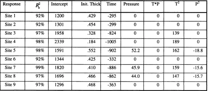
The results of regressions on the data gathered by the first experiment are summarizedt in Table 2, which shows the coefficients of each variable for the final thickness response at each of the 9 chosen sites on a wafer. As a reminder, the site map is illustrated in Figure

6. The regression package provided with Microsoft Excel Version 5.0 for Windows 3.1 was used to produce these results. Here the time units are minutes.

Response Intercept Init. Thick Time Pressure T*P T2 p2

Site 1 92% 1200 .429 -295 0 0 0 0 Site 2 92% 1301 .454 -299 0 0 0 0 Site 3 97% 1958 .328 -824 0 0 139 0 Site 4 98% 2339 .184 -1005 0 0 189 0 Site 5 98% 1591 .552 -902 52.2 0 162 -18.8 Site 6 92% 1344 .425 -332 0 0 0 0 Site 7 99% 1820 .410 -886 45.9 0 159 -15.6 Site 8 97% 1696 .466 -862 44.0 0 147 -15.7 Site 9 97% 1296 .468 -363 0 0 0 0

Table 2: Regression Coefficient Results for 9 sites

There are two main features to look for in assessing these results with respect to the RbR controller. First, how well would a first-order model of the type needed by the RbR algorithms model the responses to be controlled; second, how often and how much is back pressure a significant factor in determining the final film thickness?

*This data was later inadvertently deleted by me from the spreadsheet, and so is not available for analysis in this thesis. tThe data and regression results and details are provided in the appendix.

It appears that using a model that omits interaction and quadratic terms will have high fidelity to the behavior model obtained via linear regression. None of the responses demonstrates a statistically significant interaction between polish time and back pressure! In addition, as compared with those responses that have no squared terms, those that do also possess higher linear coefficients, and opposite-signed squared coefficients, so that qualitatively their behavior is not all that far removed from those "linear" responses.

Figure 6: Wafer Site Map

In fact, if the regression calculations are repeated for sites 3,4,5,7, and 8 with a model that has zeros for the quadratic terms, the resulting R is still over 90%, as summarized in Table 3. Since this now is a first-order model - there is still no statistically significant interaction between time and pressure - tt is the coefficients in this table that would be used by the RbR software, along with those of sites 1,2,6, and 9 from the previous table.

Unfortunately, for the RbR model, the back pressure term is only present in two responses, and its effect is small: at maximum pressure of 3 psi it predicts a relatively small change in angstroms of thickness compared to the change possible by altering polish times. Further, only the expected increase in the amount of film removed from the center is observed at all, while the predicted edge polish braking effect is not seen. This all means that the back pressure variable does not appear to provide a particularly dynamic nor general thickness variability adjustment knob to the RBR controller.

Response Intercept Init. Thick Time Pressure T*P T2 p2 Site 3 96% 1346 .429 -317 0 0 0 0 Site 4 94% 1553 .281 -312 0 0 0 0 Site 5 94% 939 .647 -310 -7.78 0 0 0 Site 7 94% 1292 .431 -305 -2.25 0 0 0 Site 8 94% 1200 .487 -322 0 0 0 0

Table 3: Linearized Regression Results

However, events in the manufacturing line caused this conclusion to be premature. First, machine maintenance records revealed that, because back pressure was not part of the production CMP recipe, it had never been calibrated since the time that the machine was originally delivered from the vendor over 18 months earlier, because no one had bothered to include it in the regular preventive maintenance worklist. So this experiment had been run with a questionable input parameter. Second, a major, annual preventive

maintenance procedure was carried out by factory technicians just a few days after this experiment was performed. Typical procedures include leveling the polish platen and similar activities that require the machine to be down for an extensive period. So the state of the machine had just been significantly altered relative to where it had just been

characterized, adding further doubt about the usefulness of the experimental results. I decided that the results were enough in question to warrant repeating the experiment, using newly-recalibrated back pressure and a freshly post-annual-preventive-maintenance CMP machine.

3.3

Experiment #2

By now the second cassette of experimental wafers had arrived, so the experiment was

simply repeated using the same randomized wafer selection as for the first cassette. Since the cassettes will not have undergone identical processing, some component of variation in the results will be due to differences between wafers processed in different cassettes, however, there is no particular need to specifically account for this difference. Table 4

summarizes the regression results; again, the RbR first-order model permitted an

excellent fit to the data, and the coefficients appear qualitatively similar to those produced by the first experiment. (In fact, the equipment technicians reported that back pressure had been only moderately out of calibration.) Unfortunately, this also means that the back pressure variable is still insufficient to permit RbR to improve the variability of the polished film thickness. Here, only one site is sensitive to back pressure, with a weak, albeit improved, effect on the result.

Response g• Intercept Init. Thick Time Pressure T*P T2 _P2

Site 1 92% 1428 .450 -465 0 0 0 0 Site 2 93% 2160 0 -435 0 0 0 0 Site 3 95% 1563 .366 -440 0 0 0 0 Site 4 97% 1473 .406 -449 0 0 0 0 Site 5 93% 1398 .429 -354 0 0 0 0 Site 6 97% 1531 .357 -484 18.1 0 0 0 Site 7 95% 1544 .356 -425 0 0 0 0 Site 8 96% 1425 .438 -390 0 0 0 0 Site 9 97% 1452 .510 -548 0 0 0 0

Table 4: Repeated Regression Results

Thus it appeared that the response surface for the CMP process was such that it was basically insensitive to back pressure.* At this stage I judged there were three main options for going forward. First, I could proceed with RbR control with the polish time control variable alone. But this would have meant only controlling mean polished film thickness, and not nonuniformity, because the RbR controller would not have sufficient degrees of freedom at its disposal to do any better. Besides, since the existing DEC CMP process control method did this already, the costs of such a demonstration would have been difficult to justify. Second, I could put the production recipe itself in bounds for

*Subsquent investigation by DEC process engineers uncovered a technical basis in the recipe for this behavior, but the details are proprietary. Generally, a number of process parameters could be set and/or interact such that they could swamp the back pressure effect.