HAL Id: emse-01233325
https://hal-emse.ccsd.cnrs.fr/emse-01233325
Submitted on 24 Nov 2015
HAL is a multi-disciplinary open access
archive for the deposit and dissemination of
sci-entific research documents, whether they are
pub-lished or not. The documents may come from
teaching and research institutions in France or
abroad, or from public or private research centers.
L’archive ouverte pluridisciplinaire HAL, est
destinée au dépôt et à la diffusion de documents
scientifiques de niveau recherche, publiés ou non,
émanant des établissements d’enseignement et de
recherche français ou étrangers, des laboratoires
publics ou privés.
Physical functions: the common factor of side-channel
and fault attacks?
Bruno Robisson, Hélène Le Bouder
To cite this version:
Bruno Robisson, Hélène Le Bouder. Physical functions: the common factor of side-channel and fault
attacks?. 2014, �10.1007/s13389-015-0111-4�. �emse-01233325�
Physical functions : the common factor of
side-channel and fault attacks ?
Bruno Robisson, H´el`ene Le Bouder
CEA-TECH / EMSE, Secure Architecture and Systems Laboratory, Centre Micro´electronique de Provence. 880 Route de Mimet, 13541 Gardanne, France
Abstract. Security is a key component for information technologies and communication. Among the security threats, a very important one is certainly due to vulnerabilities of the integrated circuits that implement cryptographic algorithms. These electronic devices (such as smartcards) could fall into the hands of malicious people and then could be sub-ject to “physical attacks”. These attacks are generally classified into two categories : fault and side-channel attacks. One of the main challenges to secure circuits against such attacks is to propose methods and tools to estimate as soundly as possible, the efficiency of protections. Numer-ous works attend to provide tools based on sound statistical techniques but, to our knowledge, only address side-channel attacks. In this article, a formal link between fault and side-channel attacks is presented. The common factor between them is what we called the ’physical’ function which is an extension of the concept of ’leakage function’ widely used in side-channel community. We think that our work could make possible the re-use (certainly modulo some adjustments) for fault attacks of the strong theoretical background developed for side-channel attacks. This work could also make easier the combination of side-channel and fault attacks and thus, certainly could facilitate the discovery of new attack paths. But more importantly, the notion of physical functions opens from now new challenges about estimating the protection of circuits.
Keywords: Differential Power Analysis, Differential Fault Analysis, Differential Behavioural Analysis, Template Attacks, Fault Sensitivity Analysis, AES128
1
Introduction
Security is a key component for information technologies and communication. Among the security threats, a very important one is certainly due to vulner-abilities of the integrated circuits that implement cryptographic algorithms to ensure confidentiality, authentication or data integrity. These electronic devices (such as smartcards) could fall into the hands of malicious people and then could be subject to “physical attacks”. These attacks are generally classified into two categories, fault and side-channel attacks and aim at bypassing the security functions, or at retrieving the details of their design, or at finding out
the manipulated data (cryptographic materials, PIN code, personal data, etc.). In the latter case and when the attacker targets cryptographic material only, we often speak of ’physical cryptanalysis’ or ’key recovering’ techniques. These techniques seem very different at first sight because they require different experi-mental methods and different algorithms. But several works have been proposed to described them in a common framework [13, 17, 6]. The aim of such frame-works is to provide strong theoretical basis but practical tools to fairly estimate the information leakage of circuits and thus increase the level of trust in such devices. But these works only cover side channel attacks. This paper describes concepts and algorithms which are common to key recovery techniques which use fault or side channel experimental set-ups. These concepts and algorithms are illustrated on the AES128 cryptographic algorithm [14].
In the first part of this article, we describe a model of circuits on which most of the attacks on AES128are based. It appears that this model uses deterministic and probabilistic functions to model the information leakage. A focus on such critical functions is provided in the second part of the article. Then, the principles of fault and side channel attacks based on this model are proposed and some illustrations are given.
2
Model of the cryptographic circuits
2.1 Observables versus internal variables
The physical attacks are based on experiments, i.e. the launches of cryptographic operations on the target with or without modifying its behaviour. During these experiments, the attacker is able to directly measure data, further called ’ob-servables’. These kinds of data are numerous :
– the electromagnetic emissions (noted EM ), current consumption (or ’power’ for short) traces (noted power ) or the signal provided by a µ-probe. – the plaintexts or the ciphertexts obtained without or with perturbations
(faulty ciphertexts).
– the behaviour (i.e. the normal or abnormal working) of the circuit in case of fault. This behaviour may be determined, for example, by comparing the correct and faulty ciphering, by detecting the start of an alarm or not, the rise time of the alarm or by detecting a more or less premature stop in computation.
– the running time. One way to measure this computation time consists in re-ducing the clock period step by step (on a specific clock cycle) and analysing the circuit’s behaviour. The step in which the behaviour of the circuit switches from normal to abnormal is considered as an indicator of the computation time. This particular step is called “fault intensity” in [12].
It should be noticed that we consider that any combination of observables or any observable obtained by applying any signal processing technique or any mathe-matical transformation (such as filtering, temporal to frequency transformation, etc.) is considered as an observable.
Opposite to the observables, the execution of a cryptographic algorithm in-volves data that cannot be directly measured by the attacker. This piece of data is called internal data in the following paragraphs. Some of these internal data are searched by the attacker and are further called ’target’ or ’secret’.
2.2 Relationships
As they are computed by, or emanate from the same circuit, variables (i.e. hidden data and observables) are related to each others. Some relationships are known by the attacker and some are not. In the physical cryptanalysis scenario (i.e. only the cryptographic materials are searched), the known relationships are generally described by an algorithm (such as a cryptographic standard) and so will further be called ’algorithmic’ relationships. In this scenario, unknown relationships are generally those which link some internal data and possibly some observables together and then will further be called ’physical’ relationships.
Known (or algorithmic) relationships In this paper, we focus on the 128-bit version of the AES standard (noted AES128). This is a standard established by the NIST [14] for symmetric key cryptography. The algorithmic relationships involved in the AES128 are now described. This algorithm ciphers a 128-bit long data (called plaintext or input ) by using a 128-bit long key to obtain a 128-bit long data (called ciphertext or output ). The encryption consists first in transforming the input data into a two-dimensional array of bytes, called the State. Then, after a preliminary bitwise XOR between the input and the key, AES128 executes 10 times a function (called round ) that operates on the State. The operations used during these rounds are the following ones:
– SubBytes (SB for short) is a non-linear transform working independently on individual bytes of the State. The result of this operation at round i is noted round[i].s box
– ShiftRows (SR for short) is a rotation operation on each row of the State. The result of this operation at round i is noted round[i].s row
– MixColumns (MC for short) is a linear matrix multiplication working on each column of the State. The result of this operation at round i is noted round[i].m col
– AddRoundKey (ARK for short) is a bitwise XOR between the State and a value k sch[i], computed from the key (according to a transform called Key Expansion which is not detailed in this paper). The result of this operation is the start of the next round noted round[i + 1].start.
The rounds are identical, except for the last one in which the MixColumns operation is skipped. At the end of the ciphering operations, the State is copied to the output.
Unknown (or physical) relationships The relationships which link some internal data and eventually some observables together have been called leakage functions in [17] for side channel attacks. To extend this notion to fault attacks, we also consider “error leakage” functions (or “error functions” for short) which formalize the relationships between some internal data and the same internal data but in the presence of perturbations. Leakage and error functions will fur-ther indifferently be called ’physical functions or ’physical relationships’. These functions deeply depend of the circuit under attack and of the experimental set-up. As they are at the heart of the physical attacks, they are detailed in the following section.
3
Models of physical functions
Except for very particular cases (such as a direct probing of an internal data), physical functions have no analytical expressions. To deal with this issue, models of these relationships have been proposed and fall into two categories. Some are ’real functions’ in the mathematical mean of the term, and some consider inputs and outputs as random variables. These two cases are respectively further be called ’deterministic’ and ’probabilistic’ physical functions. In these two cases, the models are built on the following small set of functions but note that even the more complex ones are only a model and so do not perfectly describe the real behaviour of the circuit.
3.1 Definitions
Data representation A byte B is a set of 8 bits noted {b7, . . . , b0}. We match it with B the binary value Bb= b7b6b5b4b3b2b1b0but for the sake of simplicity, B and Bb will be used indifferently. The decimal value associated with B is noted Bd (for this conversion, b0is the less significant bit).
Bit level functions The logical operations AND (symbol &), OR (symbol |) and XOR (symbol ⊕) defined on a byte are considered bitwise.
Select subset (or restriction) of bits Let B (resp. Ω) be a set of bits bi(resp. ωi). The set of bits bi of B such that ωi of Ω is equal to “1”, is noted RΩ(B). Example: if Ω = {0, 0, 1, 0, 0, 1, 0, 0}, we have Ωd= 36 and the restriction of B by R36is the set of bits {b5, b2} of B. Note that if B is constituted of N values, there are 2N − 1 possible restrictions. A restriction is said monobit when only one bit of the byte is considered. So, the monobit restrictions are R1, R2, R4, . . . , R128.
Subset of bits equal to Let Ω and B be two sets of N bits. Let M be the number of bits of the restriction of RΩ(B) and α a set of M bits. We note RΩ(B) == α the function that returns 1 when, for any bit i of RΩ(B) and α, we have RΩ(B)i== αiand returns 0 otherwise. For example, R36(B) == {0, 1} returns 1 if b5== 0 and b2== 1 and return 0 in all the other cases.
3.2 Deterministic physical functions
Deterministic leakage functions The simplest model proposed for power consumption consists in considering the value of a single bit. In this case, the leakage function is Ri with i ∈ {1, 2, 4, . . . , 128}. But more generally, side chan-nel functions are chosen as a combination of restrictions and weighted sums. For example, the number of 1 values in a binary number B is called Hamming Weight and is noted HW (B). A variation consists in considering the number of transitions between two binary values. This function, called Hamming Distance, is noted HD(B, Ω) = HW (B ⊕ Ω).
Deterministic error functions
Bit flip A fault may invert a set of bits. The function which models the bit flip is the bitwise XOR between B and Ω with Ωd∈ [1, . . . , 255]. When all the bits of the Ω are equal to 1 (resp. 0), all the bits are inverted (resp. unchanged).
Set and reset A fault which forces bits to ’0’ (resp. ’1’) is generally called a reset (resp. set ). The function which models such a reset (resp. set) is the bitwise AND (resp. OR) between B and Ω with Ωd∈ [1, . . . , 255]. A reset with Ωd = 0 returns a set of 0. A set with Ωd= 255 returns a set of 1.
Behaviour As a generalization of the set and reset models, a fault may force the bits RΩ(B) of B to some value α. In such a case, the circuit behaviour is normal only when the perturbed result is expected to be equal to α and is abnormal otherwise. Such a behaviour may be described by using the function RΩ(B) == α.
Running time (or ’fault intensity’) When the faults are created by violating the set-up time of latches, these faults may impact first the bytes which have the higher Hamming Weight or may impact first only one bit. In the first case, chip’s behaviour may be described by a Hamming Weight and in the second case by the function that selects one bit Ri with i ∈ {1, 2, 4, . . . , 128}.
3.3 Probabilistic physical functions
In this case, the input X and output Y of the physical functions are consid-ered as two discrete random variables. As observables are measured with digital equipments (such as a digital oscilloscope) and as internal data are also gener-ally organized into finite set of bits (called registers), without loss of generality, we consider that observables and internal data are discrete data. So, X and Y have respectively sample spaces SX = {0; 2M − 1} (with M being, for example, the size of a register) and SY = {0; 2N − 1} (with N being, for example, the number of bits fixed by the vertical resolution of the oscilloscope). The AES128 algorithm, considered in this article, is generally attacked thanks to a divide and conquer approach. As this method enables to recover the key byte per byte, M
is further supposed to be equal to 8. Furthermore, as most of oscilloscopes have an 8-bit vertical resolution, N is further supposed to be equal to 8. As suggested in [10], we propose to model a probabilistic relationship with a joint probability mass function (or joint pmf ). The joint pmf of the discrete variables X and Y (used to model a physical function f with domain X and co-domain Y) is noted fX,Y(x, y) = P r(X = x, Y = y) whatever x ∈ SX and y ∈ SY. Examples of such pmf are described in the next sections.
Probabilistic leakage functions Let’s consider a physical relationship which links the integer values of an 8-bit data and the current consumption measured on the circuit when it handles these values. One classical probabilistic leakage function is to consider that the current consumption of the data x is the sum of the Hamming weight of x and a Gaussian noise [5]. This assumption holds for example when the data switches from the all-zero value to the value x. It occurs, for example, during the transfer of this data on a precharged bus between the memory and the pipeline of a microprocessor. In such a case, we have f (x) = HW (x) + e with e being a normal random variable with mean 0 and a given standard deviation. The left part of the figure above describes the associated pmf (with a standard deviation of 4/10, chosen arbitrarily as an illustration). The integer values of the 8-bit data is reported in abscissa and the associated current consumption in ordinates. The darker in the Figure, the higher the probability that the circuit consumes the current of value y when the manipulated data has the value x is (shorter x ’consumes’ y). The right part of the figure is the same pmf but measured on a real component (a 32-bit unsecured up-to-date micro-controller). One can see in this very particular case that the theoretical and practical relationships fit particularly well.
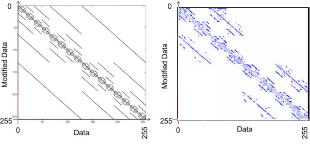
Probabilistic error functions Let’s consider a physical relationship which links the integer values of an 8-bit register and its values modified by some fault injection means. One popular model consists in considering that one out of the 8 bits of the register flips and that the probability that each of these bit flips are equal. This model will further be noted f (x) = x ⊕ Ω with Ω ∈ {1, 2, 4, . . . , 128} and (P r(Ω) = 1/8)∀Ω and be called ”monobit fault model”. Such a theoretical model is used for example in [7]. The left part of the figure above describes the associated pmf. The integer values of the 8-bit register is reported in abscissa and the associated faulted value in ordinates. The darker in the Figure, the higher the probability that x is modified into y is. The right part of the figure is the same pmf but measured on a real component by using reduction of the clock period [1]. The theoretical and experimental pmf are in this example rather distinct. In fact, in the experimental set-up, we can distinguish monobit faults but some bits appear much more easy to modify than another. In this case, the equal likelihood hypothesis is not validated.
Fig. 2. Joint pmf of the error functions : theoretical (left) and experimental (right)
4
Application to physical cryptanalysis
The physical cryptanalysis scenario (i.e. only the cryptographic materials are tar-geted) corresponds to numerous attacks proposed in the literature : µ-probing attacks, differential power analysis (with or without profiling), template attacks, differential fault analysis and safe-error attacks (among them differential be-havioural analysis and fault sensitivity analysis). All these physical attacks share the following key retrieving algorithm.
4.1 Attack path
Definition An attack path is a relationship between observables that involves the secret and that enables to recover information about it. As such attacks use a divide and conquer approach, a relationship needs to involve only a partial key (i.e. a small piece of the key). In the following paragraphs, we note
P = REL(C, F, O)
the attack path that links together the observables O and P according to the (unknown) value of the internal variables C (among them is the secret) and to a set of (unknown) physical functions F . Even if there is not always a causality relation between P and O, the observables O are further called ’stimuli’ and the observables P are called ’reactions’ or ’response’.
Examples of attack paths The attack path used in [8] and noted RELpower links the jth byte of the plain text (noted plainj), the jth byte of the first round key (noted k sch[0]j) and the power consumption measured when the computation of the jthSubBytes of the first round is performed. The algorithmic functions involved in this relationship are the SubBytes and the bitwise XOR of the AES128. The physical relationship involved links the value at the output of jth SubByte of the first round and the power consumption of the circuit when this value is computed. The associated physical function, noted f , has no analytical expression. The secret variable here is {k sch[0]j}. With
– O = {plainj}, – P = {power}, – C = {k sch[0]j},
– F = {f }, the relationship RELpower may be written : – power = fpower(SB(ARK(plainj, k sch[0]j))
Variants of this relationship are indifferently used in side-channel and fault attacks. In the first case, the measure performed in by the attacker may be an electromagnetic radiation or a signal recovered by a µ-probe. In the second case, the observables such as the behaviour or the running time are obtained by modifying the circuit’s functioning. Nevertheless, to obtain the associated relationship, the physical function fpower has only to be replaced, respectively by fEM, fµ−probe, fbehaviour or ftime.
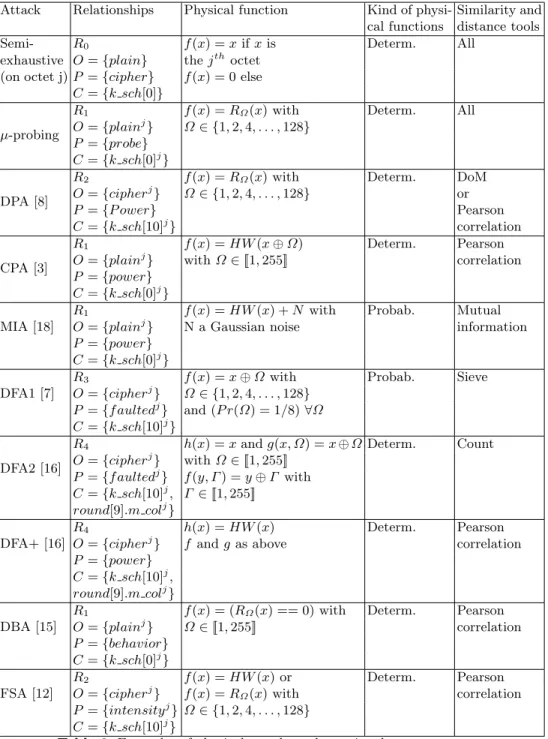
Other examples of relations widely used to break the AES128 with physical attacks are reported in the Figure 4.1. In these relations, k is the index of a byte of the State of the AES128 (so 0 ≤ k < 16) before the Shif tRow and j is the index of the same byte after this operation (so 0 ≤ j < 16). According to the notation used in the standard, k = r + 4 ∗ c with 0 ≤ r < 4 et 0 ≤ c < 4 and j = r + 4 ∗ c0 with c0 = (r − c)M odulo(4). In these relations, the functions f , g or h are leakage or error functions. Some of them will be detailed in 4.3. Variants of these relations are also proposed. They are obtained by changing the kind of the reactions.
REL0 O = {plain} P = {cipher} C = {k sch[0]} cipher = AES(plain, f (k sch[0])) REL1 O = {plainj} P = {power} C = {k sch[0]j}
power = f (round[1].startj) with
round[1].startj= SB(ARK(plainj, k sch[0]j))
Variants P = {EM } or P = {µ − probe} or P = {behaviour} or P = {time} REL2 O = {cipherj}
P = {power} C = {k sch[10]j}
power = f (round[10].startk) with
round[10].startk= SB−1(SR−1(ARK(cipherj, k sch[10]j))) Variants P = {EM } or P = {µ − probe} or P = {behaviour} or P = {time} REL3 O = {cipherj}
P = {f aultedj} C = {k sch[10]j}
f aultedj= ARK(SR(SB(f (round[10].startk))), k sch[10]j) with
round[10].startk= SB−1
(SR−1(ARK(cipherj, k sch[10]j)))
REL4 O = {cipherj}
P = {f aultedj}
C = {k sch[10]j, round[9].m colj}
f aultedj= h(ARK(round[10].s rowj0, f (k sch[10]j))) with round[10].startk= SB−1(SR−1(ARK(cipherj, k sch[10]j))) k sch[9]k0= g(ARK(round[10].startk, round[9].m colk))
round[10].s rowj0 = SR(SB(ARK(k sch[9]k0, round[9].s colk))) Variant P = {power}
Table 1. Relationships used to break the AES128with physical cryptanalysis
4.2 Key retrieving algorithm
Step 0: Notations Let’s note A a set of n variables noted {a1, a2, . . . , an}. We consider that each variable ai is discrete and has its own finite set of definition, noted Ai with cardinal |Ai|. When a variable ai takes a particular value, noted ai(j) with 0 ≤ j < |Ai|, this variable is said ’instantiated’. By extension, ˜A denotes the set of all the possible values of A. So, there are | ˜A| = |A1| ∗ |A2| ∗ . . . ∗ |An| distinct possible instances. Each of these instances is noted ˜A(j).
Step 1: Choice of the attack path Among the different relationships described in Table 1 and depending of his experimental set-up, the attacker chooses a relation P = REL(C, F, O), with C and F unknown and with O and P known by the attacker.
Step 2: Definition of the search space The attacker chooses hypotheses on the values of C and F . The set of hypothesis on the physical functions is noted ˜F
and the set of hypotheses on the internal variables is noted ˜C. The set ˜C ∗ ˜F is called the search space and has | ˜C| ∗ | ˜F | elements. This sets are chosen such that
˜
C contains C and such that at least a physical function of ˜F approximates the function F . As it is impossible to try all the possible physical functions (the set of leakage functions is infinite and the set of all the error functions for an octet is constituted of 256256 = 22048 elements), heuristics have to be used. These heuristics are based on the knowledge that the attacker has on the circuit and on his experimental set-up. In some scenarii, the attackers may take advantage of a ’profiling’ phase on a circuit identical to the circuit under attack. During such an optional phase, he is able to estimate the leakage functions (and thus refine his hypotheses). In the other cases, he models the physical functions with a priori functions detailed in 3.2.
Step 3 : Experiments The attacker performs a set of experiments to measure and record the reactions P of the circuit for different stimuli O. The stimulus used for the experiment e is noted O(e) and the reaction measured for this experiment is noted P (e). From all the set of measurements, the attacker is able to compute P r(P, O).
Step 4 : Predictions The attacker builds a set of hypothesis of relationship by replacing in REL the elements of C by all the values ˜C(i) ∈ ˜C of internal variables and the elements of F by all the physical functions ˜F (j) ∈ ˜F . Each element of this set of relationship is called ’model’ parametrized by ˜C(i) et ˜F (j) and noted M od(i, j). Then, depending of the kind of chosen physical functions (deterministic or probabilistic), two cases arise:
– Deterministic: For all the models and for each experiment e realized during the previous step, the attacker predicts the reactions noted PM od(i,j)0 (e) = REL( ˜C(i), ˜F (j), O(e)).
– Probabilistic: For all the models, the attacker estimates the probability of having the reaction and the stimuli P r(PM od(i,j)0 , O) on the all set of exper-iments.
Note that the joint probability P r(PM od(i,j)0 , O) may be also calculated in the first case (i.e. when the physical functions are deterministic). Note also that in the second case, the stimuli used to compute the joint probability do not have to be strictly identical to those used during the measurement step. The stimuli just have to have the same probability distribution.
Step 5 : Comparison between predictions and measures Then, the attacker com-pares his predictions and the measurements. According to the values of hypoth-esis, two cases arise when the relation REL has statistical properties (which is the case for those reported in Table 4.1).
1. Good hypothesis: When the physical function F could be soundly approxi-mated (or is equal in very particular cases) by a function in ˜F , then there is
an index j0 such that ˜F (j0) ' F . In this case, for i = i0, with i0 being the index of C in ˜C, the predicted reactions are ’quasi-identical’ to the measured ones for all the experiments. So, we have PM od(i0
0,j0)(e) ' P (e)∀e when the
physical functions are deterministic and P r(PM od(i0
0,j0), O) ' P r(P, O) when
the physical functions are probabilistic. In such case, the model parametrized by the key ˜C(i0) and the function ˜F (j0) ’explains the data’.
2. Bad hypothesis: On the contrary, when i 6= i0or j 6= j0, P (e) and PM od(i,j)0 (e) are not identical for all the experiments in the deterministic case and in the probabilistic case P r(PM od(i0
0,j0), O) and P r(P, O) are distinct.
Different algorithms are used to implement the comparator ' cited above (also called ’distinguisher’). In the deterministic case, ad-hoc algorithms have been proposed such as the three following ones:
– The ’sieve’ algorithm return a binary value equal to 1 if and only if PM od(i,j)0 (e) = P (e) for all the experiments. The model explains the data if and only if the return value is 1.
– The ’count’ algorithm returns the number of times that PM od(i,j)0 (e) = P (e). The higher, the better the hypothesis explains the data.
– When the possible values for the predictions are restricted to the set {0, 1}, Kocher and al. have proposed to compute the difference of the mean (’DoM’ for short) of the set of measures associated with the prediction ’1’ and the mean of the set of measures associated with the prediction ’0’ [8]. The higher, the better the hypothesis explains the data.
Other more general algorithms, based on information theory or on statistics operators have been proposed. In the deterministic case, comparing PM od(i0
0,j0)(e) '
P (e)∀e is equivalent to compare the pmf P r(PM od(i0
0,j0)) and P r(P ). In the
prob-abilistic cases, comparing if the joint pmf P r(PM od(i0
0,j0), O) and P r(P, O) are
identical, is equivalent to compare the pmf PM od(i0
0,j0)and P r(P ). So, the two
cases (i.e. probabilistic and deterministic cases) collapse. A survey of operators for comparison is available in [4]. Two of them are described below.
– As the predictions and the measures are supposed to be ’similar’, the Pear-son coefficient has been used to test the linearity between P0 and P . The coefficient returns a values between 1 and -1. The higher in absolute value, the better the model explains the data.
– As the predictions and the measures are supposed to share information, the mutual information (MI) between the random variables PM od(i,j)0 and P has also been proposed. The MI return a value between 0 and 1. The higher, the better the model explains the data.
When the good and bad hypothesis cases are distinguishable, the attacker gets information on the internal data (value of C) but also on the physical functions associated with the circuit and with the experimental set-up. Examples of instances of this key retrieving algorithm are proposed in the following section.
4.3 Illustrations
In the Table 2 are presented the different parameters defined in the framework proposed above for some well known attacks on the AES. For the 128-bit version of this algorithm, the attacker has to perform 16 times an elementary attack (which enables him to retrieve the octet j of the key).
Semi-exhaustive The principle of this (rather theoretical) attack consists in forc-ing with any fault injection mean, 15 bytes of the key to “00” and in leavforc-ing unchanged the value of the byte j. The attacker records a couple plain/cipher texts obtained in such conditions. In a second step, the attacker generates the set of 256 keys such that all the bytes of these keys are equal to “0” except the jth one which takes a value i among {0, . . . , 255}. The attacker computes, by using the AES algorithm, the cipher text obtained for each value of this set of keys hypothesis. Only one value, for example i0, explains the cipher text from the plain text. The attacker deduces that the byte j of the key is equal to i0.
µ-probing In this example, let’s suppose that the attacker targets the software implementation of the AES on a 8-bit micro-controller and that he knows exactly when the output of the S-Box of the first round of one byte of the state is moved from the processor to the memory. We also suppose that the attacker is able to measure the signal of one (and only one) wire of the data bus but that the index of this bit is unknown. In such a rather pedagogical than realistic scenario, the attacker measures one bit during each experiment, which consists in computing a cipher from a known plain text. As the index of the bit is unknown, the attack has to test 8 different physical functions, each of them being a monobit restriction that corresponds to an index of the bit in the byte. All kind of distinguisher could be used to retrieve the value of the key hypothesis.
DPA In the case of DPA, the physical function used to model the power con-sumption is a monobit restriction. So, the attacker has to test 8 possible physical functions (one for each bit) for each of the 256 values of key hypothesis. The difference of means could be used to distinguished the correct key and the false key.
CPA In the case of CPA, the attacker supposes that the power consumption depends on the SubBytes output but also on another value (which could be the previous value in the register which store the SubByte outputs). As this value is unknown, it can be seen as a parameter of the leakage function. So, the attacker has to try the 256 values of the secret key for each of these leakage functions. The distinguisher of CPA is the Pearson correlation coefficient.
MIA In the case of MIA, the attacker supposes that the power consumption depends on the SubBytes output but also on another value (as for the CPA). But the MIA takes into account an additive Gaussian noise (so the model is probabilistic). The distinguisher of MIA is the mutual information.
Attack Relationships Physical function Kind of physi-cal functions
Similarity and distance tools
Semi- R0 f (x) = x if x is Determ. All
exhaustive O = {plain} the jthoctet (on octet j) P = {cipher} f (x) = 0 else
C = {k sch[0]}
µ-probing
R1 f (x) = RΩ(x) with Determ. All
O = {plainj} Ω ∈ {1, 2, 4, . . . , 128}
P = {probe} C = {k sch[0]j}
DPA [8]
R2 f (x) = RΩ(x) with Determ. DoM
O = {cipherj} Ω ∈ {1, 2, 4, . . . , 128} or
P = {P ower} Pearson
C = {k sch[10]j} correlation
CPA [3]
R1 f (x) = HW (x ⊕ Ω) Determ. Pearson
O = {plainj} with Ω ∈ [[1, 255]] correlation
P = {power} C = {k sch[0]j} MIA [18]
R1 f (x) = HW (x) + N with Probab. Mutual
O = {plainj} N a Gaussian noise information
P = {power} C = {k sch[0]j}
DFA1 [7]
R3 f (x) = x ⊕ Ω with Probab. Sieve
O = {cipherj} Ω ∈ {1, 2, 4, . . . , 128} P = {f aultedj} and (P r(Ω) = 1/8) ∀Ω C = {k sch[10]j}
DFA2 [16]
R4 h(x) = x and g(x, Ω) = x ⊕ Ω Determ. Count
O = {cipherj} with Ω ∈ [[1, 255]] P = {f aultedj} f (y, Γ ) = y ⊕ Γ with
C = {k sch[10]j, Γ ∈ [[1, 255]] round[9].m colj}
DFA+ [16]
R4 h(x) = HW (x) Determ. Pearson
O = {cipherj} f and g as above correlation
P = {power} C = {k sch[10]j,
round[9].m colj} DBA [15]
R1 f (x) = (RΩ(x) == 0) with Determ. Pearson
O = {plainj} Ω ∈ [[1, 255]] correlation
P = {behavior} C = {k sch[0]j}
FSA [12]
R2 f (x) = HW (x) or Determ. Pearson
O = {cipherj} f (x) = RΩ(x) with correlation
P = {intensityj} Ω ∈ {1, 2, 4, . . . , 128} C = {k sch[10]j}
DFA1 The DFA proposed in [7] uses the theoretical error function described in 3.3. The distinguisher is a sieve algorithm.
DFA2 The DFA proposed in [16] use a constant error (or at least which provides a ’good repeatability’) which spreads across the key schedule. This error creates 2 faults on the State and the values of these faults are unknown by the attacker. So, he tests all the possible values of these faults (but also tests the values of the key) in order to find the model which explains the data. The distinguisher used is a count algorithm.
DFA+ The principle of the DFA+ consists in combining side channel and fault attacks. In such attack, two physical functions are used: one for the error function (a constant error such as in DFA1) and one for the leakage function (an Hamming Weight). The chosen distinguisher is the Person coefficient.
DBA The principle of the DBA consists in explaining a behaviour (i.e. the circuit works correctly or not) by using a model parametrized by the value of the key and a constant (but unknown) fault model (for example the set or the reset of some bits of the outputs of a SubByte). The distinguisher is a Person correlation. This attack is particularly effective when the circuit embeds protections against DFA.
FSA FSA consists in explaining a fault sensitivity (i.e. the behaviour of the circuit to a fault injection mean whose intensity is variable) by using a model parametrized by the value of the key and a constant (but unknown) fault model (for example an Hamming Weight or set/reset of a particular bit of the input of a SubByte). The distinguisher is a Pearson correlation.
Conclusion
We showed in this article that most side channel and fault attacks share the same principles. This merge has been made possible by extending the concept of leakage functions by the concept of error functions and by using probability mass functions to model both of them. Many possible further works have been identified : First, we plan to describe a wider set of attacks with our framework. In particular, it could be interesting to extend our approach to asymmetric cryptography (and include attacks described in [2]). Second, for a given set of models of physical functions, we could plan to formally study the attack paths and thus automatically generate new ones. Third, this work could be seen as the basis for merging the advantages of attack-specific protections to enable a more generic set of countermeasures. At last, because physical functions are at the heart of the attack, we believe that their studies are a promising way to fairly estimate the security of the device. But these studies give way to a lot of open questions:
– How to estimate the error between the model and the actual physical func-tions? This question has been covered by several articles like [6] but they will certainly have to be updated to take into account the pmf of error func-tions. Indeed, these functions have very different statistical properties than the pmf of leakage functions.
– Do some physical functions leak more information than others? Intuitively and as suggested in [9, 11], if the pmf of a physical function is the uniformly random distribution, there are certainly less risks than if the pmf of the function is one of those described in 3.3. It could be interesting to find mathematical criteria (certainly based on the measure of randomness of the pmf ) to evaluate the intrinsic leakage of physical functions.
– A corollary is how to find the critical physical functions that leak the most? In this article, we have considered that the physical functions take only one argument. But theoretically, each observable depends on all the other vari-ables. For example, an error function could depend on X, on the previous value of X but also on other observables such as the voltage, the tempera-ture and even perhaps, due to cross-talk, on many other internal variables. Thus, the number of possible physical functions appears to be tremendous. Enumerating all of them, even for a very small circuit is to our point of view, impossible. The community will have to define heuristic to find the most critical physical functions. But the use of such non exhaustive search could lead to potential undetected leakage.
In other words, from our point of view, the estimation of the information leakage of a chip is far from being solved.
Acknowledgements
The authors would like to thank D. Aboulkassimi, J.-M Dutertre, I. Exurville, J. Fournier, R. Lashermes, J.-B. Rigaud, A. Tria and Jean-Yves Zie for their contributions to this work. We would like to thank the anonymous referees and Ph. Maurine for their valuable comments and suggestions. This research is in part supported by the French government through the CALISSON 2 and the HOMERE+ projects.
References
1. Agoyan, M., Dutertre, J.M., Naccache, D., Robisson, B., Tria, A.: When clocks fail: On critical paths and clock faults. In: Gollmann, D., Lanet, J.L., Iguchi-Cartigny, J. (eds.) CARDIS. Lecture Notes in Computer Science, vol. 6035, pp. 182–193. Springer (2010)
2. Barthe, G., Dupressoir, F., Fouque, P.A., Gr´egoire, B., Zapalowicz, J.C.: Synthe-sis of fault attacks on cryptographic implementations. IACR Cryptology ePrint Archive 2014, 436 (2014)
3. Brier, E., Clavier, C., Olivier, F.: Correlation power analysis with a leakage model. In: Joye, M., Quisquater, J.J. (eds.) CHES. Lecture Notes in Computer Science, vol. 3156, pp. 16–29. Springer (2004)
4. Cha, S.H.: Comprehensive survey on distance/similarity measures be-tween probability density functions. International Journal of Mathemat-ical Models and Methods in Applied Sciences 1(4), 300–307 (2007), http://www.gly.fsu.edu/ parker/geostats/Cha.pdf
5. Chari, S., Rao, J.R., Rohatgi, P.: Template attacks. In: Jr., B.S.K., C¸ etin Kaya Ko¸c, Paar, C. (eds.) CHES ’02: Revised Papers from the 4th International Workshop on Cryptographic Hardware and Embedded Systems. Lecture Notes in Computer Science, vol. 2523, pp. 13–28. Springer-Verlag, London, UK (2002)
6. Durvaux, F., Standaert, F.X., Veyrat-Charvillon, N.: How to certify the leakage of a chip? In: Nguyen, P.Q., Oswald, E. (eds.) EUROCRYPT. Lecture Notes in Computer Science, vol. 8441, pp. 459–476. Springer (2014)
7. Giraud, C.: DFA on AES. In: Dobbertin, H., Rijmen, V., Sowa, A. (eds.) Advanced Encryption Standard - AES. Lecture Notes in Computer Science, vol. 3373, pp. 27–41. Springer (2005)
8. Kocher, P.C., Jaffe, J., Jun, B.: Differential power analysis. In: Wiener, M.J. (ed.) CRYPTO. Lecture Notes in Computer Science, vol. 1666, pp. 388–397. Springer (1999)
9. Lashermes, R., Reymond, G., Dutertre, J.M., Fournier, J., Robisson, B., Tria, A.: A dfa on aes based on the entropy of error distributions. In: Bertoni, G., Gierlichs, B. (eds.) FDTC. pp. 34–43. IEEE (2012)
10. Li, Y., Endo, S., Debande, N., Homma, N., Aoki, T., Le, T.H., Danger, J.L., Ohta, K., Sakiyama, K.: Exploring the relations between fault sensitivity and power consumption. In: Prouff, E. (ed.) COSADE. Lecture Notes in Computer Science, vol. 7864, pp. 137–153. Springer (2013)
11. Li, Y., ichi Hayashi, Y., Matsubara, A., Homma, N., Aoki, T., Ohta, K., Sakiyama, K.: Yet another fault-based leakage in non-uniform faulty ciphertexts. In: Danger, J.L., Debbabi, M., Marion, J.Y., Garc´ıa-Alfaro, J., Zincir-Heywood, A.N. (eds.) FPS. Lecture Notes in Computer Science, vol. 8352, pp. 272–287. Springer (2013) 12. Li, Y., Sakiyama, K., Gomisawa, S., Fukunaga, T., Takahashi, J., Ohta, K.: Fault sensitivity analysis. In: Mangard, S., Standaert, F.X. (eds.) Crypto-graphic Hardware and Embedded Systems, CHES 2010, Lecture Notes in Com-puter Science, vol. 6225, pp. 320–334. Springer Berlin / Heidelberg (2010), http://dx.doi.org/10.1007/978-3-642-15031-9 22, 10.1007/978-3-642-15031-9 22 13. Micali, S., Reyzin, L.: Physically observable cryptography. IACR Cryptology ePrint
Archive 2003, 120 (2003)
14. NIST: Announcing the Advanced Encryption Standard (AES). Federal Information Processing Standards Publication, n. 197 (Nov 26, 2001)
15. Robisson, B., Manet, P.: Differential behavioral analysis. In: Paillier, P., Ver-bauwhede, I. (eds.) Cryptographic Hardware and Embedded Systems (CHES), Lec-ture Notes in Computer Science, vol. 4727, pp. 413–426. Springer (10-13 September 2007), http://dx.doi.org/10.1007/978-3-540-74735-2 28
16. Roche, T., Lomn´e, V., Khalfallah, K.: Combined fault and side-channel attack on protected implementations of AES (2011), http://www.ssi.gouv.fr/IMG/pdf/DFSCA.pdf
17. Standaert, F.X., Malkin, T., Yung, M.: A unified framework for the analysis of side-channel key recovery attacks. In: Joux, A. (ed.) EUROCRYPT. Lecture Notes in Computer Science, vol. 5479, pp. 443–461. Springer (2009)
18. Veyrat-Charvillon, N., Standaert, F.X.: Mutual information analysis: How, When and Why? In: Clavier, C., Gaj, K. (eds.) CHES. Lecture Notes in Computer Sci-ence, vol. 5747, pp. 429–443. Springer (2009)