Nuclear reactor containment flows - Modelling of stably stratified layer erosion by a turbulent jet

HAL Id: cea-02509167

https://hal-cea.archives-ouvertes.fr/cea-02509167

HAL is a multi-disciplinary open access

archive for the deposit and dissemination of sci-entific research documents, whether they are pub-lished or not. The documents may come from teaching and research institutions in France or abroad, or from public or private research centers.

L’archive ouverte pluridisciplinaire HAL, est destinée au dépôt et à la diffusion de documents scientifiques de niveau recherche, publiés ou non, émanant des établissements d’enseignement et de recherche français ou étrangers, des laboratoires publics ou privés.

Nuclear reactor containment flows - Modelling of stably

stratified layer erosion by a turbulent jet

L. Ishay, G. Ziskind, U. Bieder, A. Rashkovan

To cite this version:

L. Ishay, G. Ziskind, U. Bieder, A. Rashkovan. Nuclear reactor containment flows - Modelling of stably stratified layer erosion by a turbulent jet. NURETH 16- 16th International Topical Meeting on Nuclear Reactor Thermalhydraulics, Aug 2015, Chicago, United States. �cea-02509167�

NUCLEAR REACTOR CONTAINMENT FLOWS – MODELLING OF

STABLY STRATIFIED LAYER EROSION BY A TURBULENT JET

Ishay L and Ziskind G

Department of Mechanical Engineering

Ben-Gurion University of the Negev

P.O.Box 653, Beer-Sheva 84105, Israel

ishayli@bgu.ac.il, gziskind@bgu.ac.il

Bieder U

DEN/SAC/DANS/DM2S/STMF/LMSF

CEA, Centre de SACLAY

F-91191 Gif-sur-Yvette, France

ulrich.bieder@cea.fr

Rashkovan A

Physics Department

Nuclear Research Center Negev (NRCN)

P.O. Box 9001, Beer-Sheva 84190, Israel

rashbgu@gmail.com

ABSTRACT

A number of international benchmarks were devoted to revealing the capability of CFD codes to predict the temporal evolution of the concentration and velocity fields of the nuclear reactor containment atmosphere in the course of severe accidents. In the most recent OECD/NEA international benchmark exercise on containment flows, a stably-stratified helium-air layer was eroded by a free turbulent jet coming from below. Velocity and helium concentration fields were measured in the course of the experiment. The results of the benchmark have shown that a correct prediction of the temporal development of the concentration field does not necessarily mean that the velocity field was resolved accurately as well. This can suggest that a wrongly predicted velocity field can compensate an erroneously modeled mass transport, still leading to a relatively correct concentration field.

This work examines numerically the temporal evolution of the velocity and concentration fields for the conditions of an international benchmark exercise on containment flows performed in PANDA facility at PSI, Switzerland. A number of preliminary separate effect studies are performed on the way to choosing the final modeling scheme. It is shown that k- SST models significantly overestimate the mixing rates, whereas the standard k- model overestimates the spreading of the jet and its center-line velocity decay rate. A good compromise seems to be found in modification of the C1 constant of the k- model allowing

to simulate erosion of the stratified layer by round jets more reliably.

KEYWORDS

Stable stratification, turbulent jet erosion, URANS, containment flow

1. INTRODUCTION

In the course of a loss of coolant accident (LOCA) in water-cooled reactors high temperatures can be reached in the core. The rate of oxidation reaction between the zirconium in the Zircaloy fuel cladding and steam is temperature controlled. If the fuel cladding enters a certain temperature range well above its typical operating conditions, the oxidation reaction becomes “autocatalytic,” meaning that it propagates via self-heating from the chemical reaction itself producing progressively increasing amounts of hydrogen gas. Hydrogen and steam could be released into the containment and stably stratified layers of hydrogen and air may be expected. The stratified layer can be further eroded by the later released hydrogen-steam mixed jets. The hydrogen-air mixture in the top portion of the containment can reach the flammability limits. Hence, prediction of the hydrogen concentration, which is controlled by both, molecular diffusion and erosion due to impingement of a free turbulent jet at the bottom of the stratified layer, is vital for an optimized positioning of countermeasures, like recombiners [1]. Experiments in full scale reactor

containments are not practical because of the rather big dimensions, time duration and safety reasons. On the other hand, since the course of LOCA involves important phenomena for nuclear safety, large scale experimental facilities like MISTRA [2] and PANDA were designed and built in order to get an insight into the relevant processes and to produce detailed data for validation of computational tools for prediction of hydrogen distribution in the containment.

One of the recently done large scale experiments was performed for the OECD/NEA benchmark exercise (IBE-3) in PANDA vessel, PSI, Switzerland. Due to the long transient time and the large PANDA vessel dimensions, the best applicable established turbulence models candidates for simulating the IBE-3 experiment are those based on Unsteady Reynolds Averaged Navier-Stokes Equations (URANS) and Reynolds Stress Models (RSM). Thus, the majority of the results submitted to IBE-3 were computed employing these kinds of models. It is imperative to validate the performance of the URANS-based models on a number of separate physical effects relevant to the integral problem of stratified layer erosion, in order to ensure that no error compensation occurs for the final integral situation.

As the turbulent jet issuing from a vertical pipe in the IBE-3 experimental set-up goes from positively through neutrally to negatively buoyant regimes, it is important for the candidate models to be first validated for these flow conditions. Study on RANS modeling of neutrally buoyant free round turbulent jets is reported elsewhere [3]. In the present study here, the flow and mixing in a positively buoyant jet is addressed. A number of preliminary studies on a simplified set-up are performed in order to establish the modeling approach to be used for the integral IBE-3 experiment simulations.

2. PRELIMINARY STUDIES 2.1. Positively buoyant jet

The air-helium mixture leaving the pipe in the conditions of IBE-3 is lighter than the PANDA vessel immediate environment. It is mandatory for predicting the jet flow and concentration field erosion that the selected turbulence model can capture correctly the behavior of this positively buoyant jet. Results presented in [4] are of the most cited experimental studies on vertical positively buoyant jets in the uniform, otherwise quiescent environment. The analysis of the results presented by [4] is carried out following the formulation presented in [5]. Dimensional numbers are defined for the buoyancy flux due to the jet-environment density difference in the presence of gravity. The buoyancy flux is expressed as B=g()0Q/ambient, where g is the gravitational acceleration, ()0 is the initial jet-to-environment density

difference and Q is the volumetric flow rate of the injected fluid. The momentum flux, M, is defined as a product of the jet mean velocity at the exit, w, and the volumetric flow rate: M=wQ. Combining the buoyancy and momentum fluxes, and the volumetric flow rate, the governing dimensionless number, Richardson number, Ri, can be expressed as Ri=QB1/2/M5/4. Ri characterizes the behavior of the injected

fluid. It assumes very small values for jet-like behavior and values of the order of magnitude of unity for plume-like jets. Additional dimensional relation is considered for the ratio of the momentum to buoyancy flux: lm=M

3/4

/B1/2, thus lm is a constant for a given velocity magnitude and density difference with the

units of distance. The dimensionless distance from the jet exit can be expressed as z/lm, z being the

distance from the jet nozzle exit to some location. Expressed in centimeters, lm varies from small values in

jets and exceeds 20 in plumes [4].

A wide span of initial jet velocities, nozzle diameters and ambient to jet fluid density ratios were employed in [4] in order to study the separate effect impact of the jet momentum and buoyance force on the positively buoyant jet behavior. Table I presents the experiments modeled in the present study.

Table I. Simulated experimental conditions [4]

𝑫, 𝐜𝐦 𝒘, 𝐜𝐦/𝐬 g (𝚫𝝆)𝟎 𝝆_{𝒂𝒎𝒃𝒊𝒆𝒏𝒕}, 𝐜𝐦 𝐬𝟐 𝒍𝒎, 𝐜𝐦 𝒛, 𝐜𝐦 𝑹𝒊 𝑹𝒆 EXP 17 0.75 35.128 1.08 27.54 24.6 0.0241 2635 EXP 23 0.75 31.98 5.80 10.83 59.5 0.0614 2399 EXP 25 0.75 16.237 5.80 5.50 39.9 0.1209 1218 EXP 29 0.75 47.72 0.20 87.74 73.6 0.0076 3579 EXP 32 1.25 5.845 10.71 1.88 43.6 0.5893 731 EXP 39 2 2.283 15.82 0.76 62.1 2.3191 457

Based on the geometry used in [4], a two-dimensional axisymmetric case is set. The computational domain dimensions are kept close to those used in the experiments. The original parallelepiped tank with a rectangular crossection of 1.15×1.15m is replaced by a cylindrical shape 1.15 meters in diameter. While this modification is not expected to have an appreciable impact on the results, the computational time is greatly reduced comparing with modeling the real 3D geometry.

Dilution of the ambient fluid inside the tank by positively buoyant jet is a transient process, especially at the beginning, when the concentration field changes rapidly. However, for high enough inventor of the ambient fluid, after some period of time, a quasi-steady state dilution process is expected. In all the simulated experiments listed in Table I, the quasi steady-state conditions were met after at most 70 seconds and lasted till at least 400 seconds. During this time, the velocities and concentrations changed by no more than 1.5%. It is worth to note that all the measurements reported in [4] were taken after 120 seconds. Hence, the results presented herewith were also calculated for time duration of 120 seconds. The geometry of the jet contraction nozzle or a precise velocity distribution at the inlet boundary is not reported in [4]. Uniform velocity inlet profile is assumed with a constant mean velocity,𝑤, and “pressure outlet” boundary condition is set 10 cm below the top wall. This boundary condition mimics the overflow expected due to the experimental tank fill up. The rest of the boundaries are defined as non-slip walls. The solution is initialized with the tank containing the denser fluid, while the lower density jet is injected upward.

The numerical approach uses in the FLUENT calculation is as follows. The pressure velocity coupling is by SIMPLE algorithm, the transient formulation is a first order implicit scheme with a constant time step of 0.01 sec. STANDARD pressure interpolation scheme is employed [6]. The spatial discretization

gradient is least squares cell based, the pressure discretization is PRESTO. A second order upwind formulation is set for the convection term in the conservation equations. The absolute criteria for convergence are 10-6 for all the conservation equations besides the energy equation for which a value of 10-9 is set. The maximal iterations' number per time step is set to 200.

Several RANS turbulence models are employed in the present study. Both, eddy viscosity models, standard k- model with C1 of 1.44 (standard k-) and 1.6 (modified k-), and k- SST model, and

second-moment closure, -based Reynolds Stress Model (RSM), were used. The models are described elsewhere [3]. Species transport equation is solved along with the continuity, momentum, energy and turbulent stresses conservation equations. Molecular diffusivity value of D=1.4·10-10m2/s [7] was used. The concentration field in a turbulent fluid flow is evaluated by the solution of the convection-diffusion equation, where the turbulent mass flux is calculated using the turbulent Schmidt number, Sct, defined as

a ratio of the turbulent viscosity to the turbulent mass diffusivity. The sensitivity of the concentration and velocity fields to the value of Sct is discussed in section 2.2.4 of the present study.

The computational grid is built using quadratic cells. Mesh refinement is employed at the velocity inlet and pressure outlet boundaries. The growth rate at these boundaries is 1.05 and the total number of computational cells in the domain is 11,575. In order to verify the grid convergence, the base grid is adapted in FLUENT, by halving each cell, in two directions, into four cells. This procedure was employed twice. Hence, the total number of cells was 46,300 for the first adaption, and 185,200 for the second one. The mesh containing 46,300 cells exhibited a converged solution and is used for the calculations reported herewith.

Table II presents the results of the center-line non-dimensional velocity and concentration at a specific location of experiment 23 (see Table I). Results obtained with the four turbulent models are presented. As it is seen from the data presented in Table II, both the modified k- and -based RSM models overpredict the momentum flux decay rate, as opposed to the standard k- and k- SST, which underpredict it by almost the same margin. The calculated center-line concentration decay rates are considerably closer to the measured ones with the modified k- and -based RSM models. It is worth to note that the

concentration decay rates are overpredicted by about 50% with standard k- and k- SST. As it was shown in [3], the modified k- and -based RSM models also performed better in the case of the neutral round jet simulation comparisons with experiments reported in [8]. It has to be mentioned however, that the centre-line velocity decay rate was over-predicted by the -based RSM model for the neutral round jet.

Table II. Non-dimensional velocity and concentration for experiment 23.

EXP 23 k-, C1=1.6 k-, C1=1.44 k-, SST RSM, C1=1.6

M1/2_{/(zw) 0.0711 0.0627 0.0787 0.0769 0.0632}

(C0/cc)Q/(zM1/2) 0.2077 0.2195 0.3247 0.2961 0.1822

It was decided to use the modified k- model to analyse the other positively buoyant jet experiments listed in Table I. Figure 1 (left) shows the computed velocity decay rate for the six analysed experiments. The dashed lines represent the span of experimental results. It can be concluded that a marginal over-prediction in the velocity decay rate can be seen for all the experiments being lower for the 17th and the 29th. These two experiments were performed with the lowest Ri studied – see Table I.

Figure 1. Left: jet axis non-dimensional mean velocity decay. Right: jet axis non-dimensional mean concentration decay.

Figure 1 (right) shows the centre-line concentration decay rate for the six experiments modelled in the present study. As it is seen from Figure 1 (right), the calculated concentration decay rates are within the experimentally observed results span. No appreciable distinction between the experiments with different Ri can be seen in concentration decay rates, opposed to the behavior of the velocity decay rates discussed above.

2.2. Comparative study of mixing in the PANDA facility

The following section presents the results of the two dimensional simulations of erosion of the stably stratified helium-air layer by a vertical round jet. The conditions of the simulations were chosen as to fit closely the geometry and the initial conditions of the IBE-3 experiment.

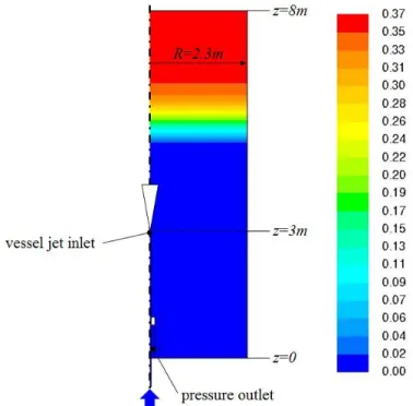
Figure 2. PANDA vessel IBE-3 set-up [1].

10-1 100 101 102 10-2 10-1 100 z/l m M 1/ 2 /(zw) 10-1 100 101 102 10-1 100 101 z/l m (C 0 /cc )Q/(z M 1/ 2 ) simulation of EXP17 simulation of EXP23 simulation of EXP25 simulation of EXP29 simulation of EXP32 simulation of EXP39 simulation of EXP17 simulation of EXP23 simulation of EXP25 simulation of EXP29 simulation of EXP32 simulation of EXP39

The PANDA vessel used for IBE-3 has a cylindrical form without partitions. As shown in Figure 2, the height of the vessel is about 8 meters and vessel diameter is 4 meters. The air-helium mixture jet is introduced into the vessel through the eccentrically located pipe. Additional details can be found in publications that summarize the experimental conditions [9] and the comparison of the submitted results with the measurements [10].

2.2.1. Analysis of the round jet

Figure 3 presents the 2D axisymmetric geometry of the simulations performed in the present study along with the initial helium mole fraction distribution. It has to be stressed that the results of the 2D

axisymmetric studies presented hereafter are not meant to be compared to the full 3D experimental values obtained during IBE-3. The aim of this preliminary study is to compare the impact of different turbulent models parameters on the calculated helium concentration and velocity fields.

The following parameters of the experiment were conserved [9]: vessel geometry, initial helium

concentration distribution, the jet vessel inlet vertical location and the inlet pipe geometry as well as the jet inlet conditions. The length of the inlet pipe is chosen such as to provide the fully developed flow conditions in the limits of the models used. The length of about 100 hydraulic diameters is set for the hydraulic flow development. The analyzed turbulence models are limited to those employed in the positively buoyant jet momentum and species transport as presented above. The value of Sct is set to 0.7.

Figure 3. Computational domain and initial helium distribution for the preliminary studies.

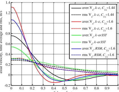
Figure 4 presents the velocity profiles after 110 seconds of the transient. The modified k- model is used as the reference result as this model was able to predict correctly not only the center-line velocity and concentration decay rates in positively buoyant jet (see section 2.1 above), but also the axial velocity and the turbulent Reynolds stresses radial distribution for the neutral round jet [3]. These turbulent stresses were computed using the Boussinesq approximation for all cases except RSM model.

Figure 4. Radial distribution of the average and rms jet center line axial velocities at 110 seconds. Results for z=5.1m (see Figure 3).

Of the four models tested, k- SST resulted in a highest velocity decay rate. One could expect the mixing rates to be the highest for the modified k- model and the lowest for k- SST in the convection dominated regions. These regions are expected to be located in the lower part of the stratified helium-air layer. The radial spread of the axial velocity seems to be of a comparable value for k- SST and -based RSM. Results obtained with the modified k- model exhibit the lowest spread and the standard k- model shows the highest spread of the four models employed.

2.2.2. Analysis of the helium erosion

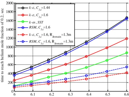
As helium concentration along the jet center-line was measured along with the velocity field during the IBE-3 experiment, the 2D axisymmetric set-up can be used to compare the turbulence model impact on the helium mole fraction distribution in the domain. The comparison between the models is presented in terms of the time needed for the helium mole fraction to drop to 0.2 at a number of probe points located along the jet axis. The same probes locations along the jet axis as in IBE-3 are used [9]. Figure 5 presents the results of helium mixing along the jet axis as calculated using different models.

As it is seen from Figure 5 the qualitative form of the mixing process temporal evolution is similar for all the models presented. The behavior of the mixing rates for the two variants of the k- model and the  -based RSM model follows the reasoning explained earlier: the higher the velocity decay rate the lower the mixing rate. The helium mole fraction drops faster for the modified k- model. It should be reminded that the modified k- model generally outpeformed its counterparts for the neutral [3] and positively buoyant jets (see section 2.1). The difference in the mixing rates between the standard k- and that for  -based RSM is negligible. In order to emphasize the sensitivity of the results to the domain geometry the modified k- and -based RSM models were applied additionally for the domain of 1.3 meters radius instead of 2.3 meters. This reduction of the domain increases significantly the mixing rates.

0 0.1 0.2 0.3 0.4 0.5 0.6 0.7 0.8 0.9 1 -0.2 0 0.2 0.4 0.6 0.8 1 1.2 1.4 radial coordinate, m a x ia l v e lo c it y , ti m e a v e ra g e a n d rm s, m /s aver.V z, k-, C1=1.44 rms V_z, k-, C 1=1.44 aver.V_z, k-, C 1=1.6 rms V z, k-, C1=1.6 aver.V_z, k-SST rms V_z, k-SST aver.V_z, RSM, C 1=1.6 rms V z, RSM, C1=1.6

Figure 5. Helium mixing rate – turbulent model impact. Time to reach helium mole fraction of 0.2.

The over-prediction of the mixing with k- SST model as compared to those obtained with the other three models used is discussed in the following section.

2.2.3. Evaluation of the k- SST model

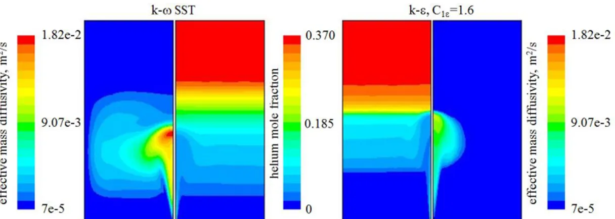
The ranking procedure of the participants of the IBE-3 benchmark included the comparison of calculated and measured velocity, temperature and concentration fields [9]. The three participants who employed k- SST model were ranked second to fourth in the global ranking. For a number of these submissions the velocity magnitude was under-predicted by 30 to 50% for 1213 and 1795 seconds; however, mixing rate was over-predicted for the same calculations [9]. The k- SST model exhibits trends similar to those reported for IBE-3 as can be seen from the velocity field of Figure 4 and helium mixing rate shown in Figure 5. While velocity decay rates are being predicted as the highest of the four models tested, the time for the helium mole fraction to drop to the value of 0.2 was the lowest. One of the possible reasons for predicting high helium mixing rates can be the high calculated values of the effective turbulent mass diffusivity that is related directly via the constant Sct to the calculated turbulent viscosity. Figure 6

presents the contours of the effective (sum of molecular and turbulent contributions) mass diffusivity and helium mole fraction for k- SST and the modified k- model at 110 seconds.

It is seen from helium distribution in Figure 6 that the rate of mixing is higher for the k- SST model throughout the whole computational domain. The mixing in the parts of the domain not effected directly by the jet momentum is controlled by the turbulent and molecular mass diffusion. The high turbulent mass diffusivity predicted by k- SST model is propagated all the way towards the vessel vertical wall whereas the turbulent mass diffusivity predicted by the modified k- model remains in the jet impact zone.

Based on the calculations presented above it is believed that the more consistent results in terms of the mutual effect of the velocity and the concentration fields are expected when the modified k- rather than k- SST model is employed. 6 6.1 6.2 6.3 6.4 6.5 6.6 0 200 400 600 800 1000 1200 1400 1600 1800 2000 vertical coordinate, m ti m e t o re a c h h e li u m m o le fra c ti o n o f 0 .2 , se c k-, C1=1.44 k-, C_1=1.6 k-, SST RSM, C_1=1.6 k-, C_1=1.6, R_domain=1.3m RSM, C 1=1.6, Rdomain=1.3m

Figure 6. Effective mass diffusivity (outer contours) and helium mole fraction (inner contours) for 110 seconds. Results for k- SST and k- model with C=1.6.

It should be stressed though that the results are expected to be dependent on whether the original k- SST formulation [12] or buoyancy corrected equations for turbulent kinetic energy and specific dissipation rate are employed – see [13] for the way the buoyancy terms in k- SST model are treated in ANSYS-CFX code.

2.2.4. Influence of the turbulent Schmidt number

All the models used in this study and those mostly used by the participants of the IBE-3 incorporate the simple gradient diffusion assumption in calculating the turbulent mass fluxes. In this approach, the turbulent mass flux is proportional to the turbulent mass diffusivity and the time average concentration gradient. The turbulent mass diffusivity is usually taken as isotropic even for the RSM model where the differential transport equations are solved for each turbulent stress. The turbulent mass diffusivity is calculated based on the analogy assumption between the momentum and the mass transfer, being equal to the ratio of the turbulent viscosity to Sct. The value of Sct used by the participants of IBE-3 varied from

0.7 to 1 [9]. The justification of using specific value Sct is questionable as it varies from one flow

situation to another and also throughout the flow field [3].

Figure 7. Sct impact for the modified k- model. Left: time for helium concentration to drop to 0.2. Right: velocities at z=6.11m for 715 seconds into the transient.

6 6.1 6.2 6.3 6.4 6.5 200 300 400 500 600 700 800 900 1000 1100 axial coordinate, m tim e to reach heli um mol e fracti on of 0. 2, sec 0 0.2 0.4 0.6 0.8 1 -0.2 -0.1 0 0.1 0.2 0.3 0.4 0.5 radial coordinate, m axial velo city , tim e averag e and rms , m/s Sc t=0.5 Sc t=0.7 Sc t=0.9 aver.V_z, Sc t=0.5 rms V_z, Sc t=0.5 aver.V_z, Sc t=0.7 rms V z, Sct=0.7 aver.V_z, Sc t=0.9 rms V z, Sct=0.9

Obviously, for the same turbulent viscosity predicted, higher values of Sct will generally lead to a lower

mixing rate and vice versa. Figure 7 (left) presents the results of helium mixing temporal evolution using the modified k- model and three values of Sct. The increase in Sct from 0.5 to 0.9 yields for 6 and 6.5

meters about 80 and 150 seconds respectively faster time for the helium concentration to drop to a mole fraction of 0.2.

As the problem of stratified layer erosion by turbulent jet is of a coupled momentum-mass transfer nature, different helium concentration profiles invoke differences in velocity fields. Figure 7 (right) presents the radial distribution of the axial average and the rms velocities at 715 seconds and at the elevation of 6.11 meters. The center-line velocity decay follows the predicted trend: the increase of Sct from 0.5 to 0.9

amplifies the axial velocity decay by about 10%. Helium mixing for the time and location presented in Figure 7 (right) is expected to be convection controlled. Hence, an accurate prediction of the flow velocity field is expected to be of decisive impact on the helium distribution. Although Sct can be used to fine tune

the calculation to reproduce an experiment, it cannot be used to compensate a known shortcoming of turbulence models due to its limited influence.

3. THE PANDA MIXING OECD/NEA BENCHMARK IBE-3

As it was shown in section 2, the modified k- and -based RSM models exhibited similar results in the validation studies on the positively buoyant jet. On the other hand, for simulations performed with

conditions similar to the IBE-3 using axisymmetric set-up, the -based RSM model predicted much slower mixing rates than the modified k- model. Those rates were very close to the ones predicted with the standard k- model. Reminding that mixing rates predicted with the standard k- in simulating LOWMA-3 MISTRA facility experiment [11] were much lower than the experimentally observed ones, it was decided to use the modified k- for the IBE-3 experiment simulation.

Selected time-dependent measurements for mass concentration by mass spectroscopy (MS) instruments were made available for comparison at 30 locations in the PANDA vessel [9]. The concentration values at four characteristic locations are compared in this paper, three in the center line of the jet (MS_2, MS_3 and MS_5) and one at a lower location outside of the jet (MS_14). Additionally, the vertical component of the jet velocity was measured at specific times along three horizontal lines. Precise information on the locations of concentration probes and velocity measurements can be found in [9].

The method to simulate the erosion of stratified layers of light gases located in test containments has been analyzed in the previous sections and in [11] for the MISTRA facility of the CEA. This method, which has been found to be code and numerical scheme independent [3], is now applied to the IBE-3 by using the CEA in-house code Trio_U [14]. Trio_U is a CFD code developed for strongly unsteady, low Mach number, turbulent flows in complex geometries. The code is especially designed for calculations on tetrahedral grids of several hundreds of millions of nodes. The platform independent code is based on an object-oriented, intrinsically parallel approach and is coded in C++. A hybrid Finite Volume Element method (FVE) is applied [15] to discretize the conservation equations. This method approximates a continuous problem by a discrete solution in the space of the finite elements by maintaining the balance notation of finite volumes. The main unknowns as velocity and scalars (e.g. temperature and

concentration) are located in the center of the faces of an element (P1NC). For the application presented here, the pressure is discretized in the center of an element (P0) as in the well-known element

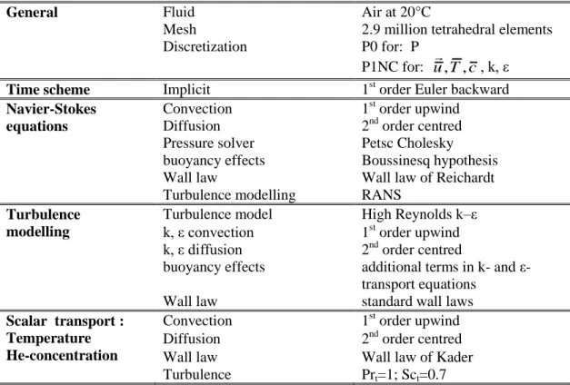
of Crouzeix-Raviart [15]. The gravity is projected along the faces of an element to avoid spurious velocity modes. An implicit velocity projection method is used to assure the mass conservation. Turbulence is treated with the modified k- model. The complete numerical scheme used for the PANDA calculation is summarized in Table III.

Table III. Fundamental numerical scheme used for the PANDA calculation

General Fluid Air at 20°C

Mesh 2.9 million tetrahedral elements Discretization P0 for: P

P1NC for: u,T,c, k, ε

Time scheme Implicit 1st order Euler backward

Navier-Stokes Convection 1st order upwind

equations Diffusion 2nd order centred

Pressure solver Petsc Cholesky buoyancy effects Boussinesq hypothesis

Wall law Wall law of Reichardt

Turbulence modelling RANS

Turbulence modelling

Turbulence model High Reynolds k–ε k, ε convection 1st order upwind k, ε diffusion

buoyancy effects Wall law

2nd order centred

additional terms in k- and ε-transport equations

standard wall laws

Scalar transport : Temperature He-concentration

Convection 1st order upwind Diffusion 2nd order centred

Wall law Wall law of Kader

Turbulence Prt=1; Sct=0.7

A pure tetrahedral mesh of 2.9 million control volumes has been created with ICEMCFD. Despite the profound analysis of modelling round jets by the modified k- model and the successful prediction of the erosion of a stratified layer in the MISTRA facility [3], this calculation has failed in the blind PANDA benchmark (user u1 in [9]). The predicted jet velocity in the impact zone was overestimated and, as a consequence, the calculated jet penetrated too deeply into the stratification layer and eroded the stratification layer too rapidly.

The turbulent viscosity has been limited in the MISTRA calculation [2] to 10-3 m²/s, in order to avoid numerical instabilities when the jet hits for the first time the stratification layer. During the transient, the turbulent viscosity was found to be by far below this threshold. The same limitation has been used for the blind PANDA calculation submitted to IBE-3 [11]. Posttest analysis of the PANDA experiment has shown that the turbulent viscosity reaches 4.10-3 m²/s in the impact zone of the jet. The limitation of the turbulent viscosity to 10-3 m²/s leads to an overestimation of the penetration of the turbulent jet into the stratification layer. Overestimation of the jet penetration into the stratified layer is expected to cause abnormally high mixing rates.

The IBE-3 simulation has been repeated after the release of the experimental data without limiting the turbulent viscosity. The comparison of the vertical velocity at the three elevations is shown in Figure 8. The profiles of the benchmark calculation and the posttest calculation are compared for 4 times with the experimental values. The center of the injection line is located at the radial position of 650 millimeters. This comparison confirms the good performance of the modified k- model in predicting the spatial evolution of round jets, even in the impact zone with the helium stratification.

Figure 8. Comparison of the vertical velocity at three elevations and 4 times. Black line – benchmark submission. Red line – corrected results. Blue dots – IBE-3 measurements.

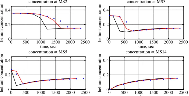
The global mixing in the PANDA vessel was evaluated by the helium concentration time history at 30 measurement positions distributed over the entire vessel [9]. Numerous positions along the injection line allowed the monitoring of the erosion of the stratification by the jet. The temporal course of the

concentration is shown in Figure 9 for four representative locations. It is evident that the benchmark submission significantly overestimates the erosion along the center-line of the jet (MS_2, MS_3 and MS_5); the corrected posttest calculation gives a much better evolution of the erosion along this line.

Figure 9. Comparison of the concentration course at four representative elevations; Legend as in Figure 8. -1200 -1000 -800 -600 -400 -200 0 0.5 1 1.5 x-coordinate, mm ax ial v el o ci ty , m/ s Hvy-1 -1200 -1000 -800 -600 -400 -200 0 0.5 1 x-coordinate, mm ax ial v el o ci ty , m/ s Hvy-2 -1200 -1000 -800 -600 -400 -200 0 0.5 1 x-coordinate, mm ax ial v el o ci ty , m/ s Hvy-3 -1200 -1000 -800 -600 -400 -200 0 0.5 1 x-coordinate, mm ax ial v el o ci ty , m/ s Hvy-5 0 500 1000 1500 2000 2500 0 0.2 0.4 time, sec h el iu m co n cen trat io n concentration at MS2 0 500 1000 1500 2000 2500 0 0.2 0.4 time, sec h el iu m co n cen trat io n concentration at MS3 0 500 1000 1500 2000 2500 0 0.2 0.4 time, sec h el iu m co n cen trat io n concentration at MS5 0 500 1000 1500 2000 2500 0 0.2 0.4 time, sec h el iu m co n cen trat io n concentration at MS14

At the lower location (MS_14), the temporal increase in the helium concentration is essentially a function of the helium injection; the vessel is rapidly filled up with helium that comes mainly from the injection line. As a consequence, these points are not affected by the overestimation of the erosion in the

calculations submitted to IBE-3 benchmark

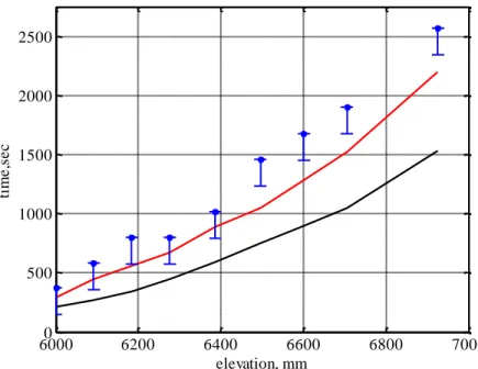
The time when the concentration measured at nine elevations along the center line of the jet drops below 0.2 is shown in Figure 10. This time is called quench time. As the scanning time of concentration measurement was 226 seconds, the maximal uncertainty of the quench times is negative (-226 seconds), i.e. the drop below 0.2 can only occur earlier than given in Figure 10 [9]. This uncertainty is also shown in Figure 10. The quench times calculated with the proposed k- modelling approach is given in

comparison with the experiment and the blind benchmark submission.

Figure 10. Time when the concentration drops at certain elevations below 0.2. Legend as in Figure 8.

This comparison shows a reasonable performance of the proposed modelling approach to simulate the PANDA experiment. Not only the predicted quench times are close to the measured ones, but also the vertical velocity profiles presented in Figure 8 are in good accordance with the experiment.

4. CONCLUSIONS

This study presents the results of a numerical simulation of the erosion process of a stably stratified layer by a vertical turbulent round jet in a large vessel. The conditions of the simulations were such that the jet entering the vessel goes from positively, through neutrally, to negatively buoyant regimes. Various RANS models were used for validation tests of the simulation results against the experiments reported in the literature for a positively buoyant jet. Both velocity and concentration fields were compared with their measured counterparts. It is concluded that the k- model and the -based RSM both with the C1 constant

of 1.6 result in an acceptable level of accuracy as compared with the experiments.

Based on preliminary separate effect studies on positively and neutrally buoyant round turbulent jets the modeling approach was formulated. The simulation results of the concentration and velocity fields were

60000 6200 6400 6600 6800 7000 500 1000 1500 2000 2500 elevation, mm ti m e ,s e c

compared to those measured in the course of the third international benchmark exercise performed in PANDA vessel at PSI, Switzerland. The comparison of both fields showed satisfactory results. It has to be stressed the correct calculations of both, the concentration and the velocity fields, is imperative in order to confidently predict the mixing in a real-size containment atmosphere for a wide range of the initial and operating conditions.

REFERENCES

1. C. Jakel, S. Kelm, E-A. Reinecke, K. Verfondern and H-J. Allelein, "Validation strategy for CFD models describing safety-relevant scenarios including LH2/GH2 release and the use of passive auto-catalytic recombiners," International Journal of Hydrogen Energy, 39, pp. 20371-20377 (2014). 2. Studer E., Brinster J., Tkachenko I., Mignot G., Paladino D. and Andreani M., "Interaction of a light

gas stratified layer with an air jet coming from below: Large scale experiments and scaling issues," Nuclear Engineering and Design, 253, pp. 406-412 (2012).

3. L. Ishay, U. Bieder, G. Ziskind and A. Rashkovan, "Turbulent jet erosion of a stably stratified gas layer - LOWMA-3 experiment simulation," submitted to Nuclear Engineering and Design, 2015. 4. P.N. Papanicolaou and E.J. List, "Investigations of round vertical turbulent buoyant jets," Journal of

Fluid Mechanics, 195, pp 341-391 (1988).

5. H.B. Fischer, E.J. List, R.C.Y. Koh, J. Imberger and N.H. Brooks, Mixing in Inland and Coastal Waters, Academic Press (1979).

6. C.M. Rhie and W.L. Chow, "Numerical study of the turbulent flow past an airfoil with trailing edge separation," AIAA Journal, 21(11), pp. 1525-1532 (1983).

7. L.A. Woolf, "Isothermal diffusion measurements on the systems sodium chloride, water-pentaerythritol and water-pektaerythritol-sodium chloride at 25oC," Journal of Physical Chemistry, 67

(2), pp. 273–277 (1963).

8. G. Xu and R.A. Antonia, "Effect of different initial conditions on a turbulent round free jet," Experiments in Fluids, 33, pp. 677-693 (2002).

9. M. Andreani, A. Badillo and R. Kapulla, "Synthesis of the OECD/NEA-PSI CFD benchmark exercise," Proceedings of CFD4NRS Conference, Zurich, Switzerland, September 9-11, 2014. 10. R. Kapulla, G. Mignot, S. Paranjape, L. Ryan and D. Paladino, "Large Scale Gas Stratification

Erosion by a Vertical Helium-Air Jet," Science and Technology of Nuclear Installations, 2014. 11. L. Ishay, G. Ziskind, A. Rashkovan, U. Bieder and J. Brinster, Simulation of LOWMA-3 MISTRA

experiment, Proceedings of CFD4NRS conference, Sep 2014, Zurich, Switzerland.

12. F.R. Menter, "Two-equation eddy-viscosity turbulence models for engineering applications," AIAA Journal, 32, pp. 1598-1605 (1994).

13. ANSYS CFX-Solver Theory Guide, Chapter 2.2.2.4, Release 15.0, November 2013. 14. Trio_U code homepage: http://www-trio-u.cea.fr