HAL Id: inria-00070642
https://hal.inria.fr/inria-00070642
Submitted on 19 May 2006
HAL is a multi-disciplinary open access
archive for the deposit and dissemination of
sci-entific research documents, whether they are
pub-lished or not. The documents may come from
teaching and research institutions in France or
abroad, or from public or private research centers.
L’archive ouverte pluridisciplinaire HAL, est
destinée au dépôt et à la diffusion de documents
scientifiques de niveau recherche, publiés ou non,
émanant des établissements d’enseignement et de
recherche français ou étrangers, des laboratoires
publics ou privés.
Modelizing, Predicting and Optimizing Redistribution
between Clusters on Low Latency Networks
Frédéric Wagner, Emmanuel Jeannot
To cite this version:
Frédéric Wagner, Emmanuel Jeannot. Modelizing, Predicting and Optimizing Redistribution between
Clusters on Low Latency Networks. [Research Report] RR-5361, INRIA. 2004, pp.14. �inria-00070642�
ISSN 0249-6399
ISRN INRIA/RR--5361--FR+ENG
a p p o r t
d e r e c h e r c h e
THÈME 1
INSTITUT NATIONAL DE RECHERCHE EN INFORMATIQUE ET EN AUTOMATIQUE
Modelizing, Predicting and Optimizing Redistribution between
Clusters on Low Latency Networks
Frédéric Wagner — Emmanuel Jeannot
N° 5361
Unité de recherche INRIA Lorraine
LORIA, Technopôle de Nancy-Brabois, Campus scientifique, 615, rue du Jardin Botanique, BP 101, 54602 Villers-Lès-Nancy (France)
Téléphone : +33 3 83 59 30 00 — Télécopie : +33 3 83 27 83 19
Modelizing, Predicting and Optimizing Redistribution between Clusters
on Low Latency Networks
Frédéric Wagner
∗, Emmanuel Jeannot
Thème 1 — Réseaux et systèmes Projets Algorille
Rapport de recherche n° 5361 — Novembre 2004 —14 pages
Abstract: In this report we study the problem of scheduling messages between two parallel machines connected
by a low latency network (LAN for instance). The problem of scheduling messages appears in code coupling applications when each coupled code has (at a given state of the simulation) to redistribute the data through a network that cannot handle all the communications at the same time (the network is a bottleneck). We compare two approaches. In the first approach no scheduling is performed. Since all the messages cannot be transmitted at the same time, the transport layer has to manage the congestion (we call this approach the brute-force approach). In the second approach we use two higher-level scheduling algorithms proposed in our previous work [14] called GGP and OGGP. We propose a modelization of the behavior of both approaches and show that we are able to accurately predict the redistribution time with or without scheduling. Although, when the latency is low, the transport layer is very reactive and therefore able to manage the contention very well, we show that the redistribution time with scheduling is always better than the brute-force approach (up to 30%).
Key-words: Code-coupling, cluster computing, message scheduling, modelization
Modélisation, prédiction et optimisation de redistributions entre grappes
d’ordinateurs à travers un réseau à faible latence
Résumé : Nous étudions dans ce rapport le problème de l’ordonnancement de messages entre deux machines
parallèles connectées par un réseau à faible latence (un LAN par exemple). Ce problème apparait pour les appli-cations de couplage de code, lorsque chaque application a, à un moment donné de la simulation, à redistribuer des données à travers un réseau ne pouvant pas effectuer toutes les communications simultanément (le réseau est un goulot d’étranglement). Nous comparons deux approches. Avec la première, aucun ordonnancement n’est effectué. Comme il n’est pas possible de transmettre tous les messages en même temps, la couche trans-port est chargée de gérer au mieux la congestion du réseau (nous appellons cette approche, approche par force brute). Avec la seconde approche, nous utilisons deux algorithmes d’ordonnancement de plus haut niveau, GGP et OGGP, proposés dans nos travaux précédents [14]. Nous proposons une modélisation du comportement de ces deux approches et montrons que nous somes capables de prédire de manière précise le temps requis pour une redistribution, qu’elle soit effectuée avec ou sans ordonnancement. Bien que, comme la latence est faible, la couche transport soit très réactive et donc capable de gérer de manière efficace la contention, nous montrons que le temps obtenu lors d’une redistribution ordonnancée est toujours meilleur qu’une redistribution par force brute (jusqu’à 30%).
1 Introduction
Code coupling applications (such as multi-physics simulations) are composed of several parallel codes that run concurrently on different clusters or parallel machines. In multi-physics simulations each code has in charge one part of the simulation. For instance simulating the airflow on an airplane wing requires to simulate fluid mechanics phenomena (the air) with solid mechanic one (the wing). In order for the simulation to be realistic
each simulation code need to exchange data. This exchange of data is often calleddata redistribution. This part of
the simulation needs to be optimized because some important time is spent doing these communications. The data redistribution problem has been extensively tackled in the literature [1, 2, 6, 7, 10]. However in these works the redistribution takes place within the same parallel machine. In the context of code-coupling, several machines are involved and therefore the redistribution must take place between two different machines through a network. In many cases this network is a bottleneck because the aggregate bandwidth of network cards of each nodes of each parallel machines exceeds the bandwidth of the network that interconnect these two machines (think for instance of two clusters with 100 nodes each and 100 MBit cards interconnected by a 1 Gbit network).
In case the network is a bottleneck it is required to schedule the messages exchanged between both machines. This scheduling can be performed either at the transport level or at the application level. The transport layer has in charge the control of the congestion and therefore can schedule the messages (at a fine grain level). In our previous work [5, 14] we have proposed several application-level messages scheduling algorithm for the redistribution problem between clusters when the network is a bottleneck. We have shown that this problem is NP-complete and the proposed algorithms (called GGP and OGGP) always find a schedule at most twice as long as the optimal one.
In this report we study the problem in the context of a low latency network (LLN), such as LAN. In LLN, the reactivity of TCP is almost perfect and the transport layer gives very good performances. In this case a naive solution that let the transport layer schedule the messages (called the brute-force approach) should behave very close to the optimal and yield to performance similar to an application-level scheduling of the message. LLN are therefore the worst-case scenario for the (O)GGP algorithms.
We provide a modelization of the behavior of TCP for the data redistribution problem as well as of (O)GGP. We compare two ways of predicting the data redistribution time. One is based on an inferior bound easily derived from the redistribution pattern, the other is based on the analysis of the pattern and our modelization of the plat-form. We show that the prediction based on the inferior bound is accurate only if the pattern has certain property whereas our modelization and pattern analysis algorithm give very accurate redistribution time either for the brute-force approach or for the (O)GGP algorithms. Furthermore we compare the performance (O)GGP against the brute-force approach. We show that even if the reactivity of transport-layer is perfect, (O)GGP algorithms always outperform the brute-force approach (up to 30%).
2 Data Redistribution
2.1
Modelization
1’ 2’ 3’ 1 4 0 7 2 5 3 0 3 2 5 0 1 1’ 2 2’ 3 3’ 4 7 5 3 2 5Figure 1.A Communication Matrix Seen as a Bipartite Graph
Let us consider an application running on two clusters connected by a low latency network (for instance a LAN). This application can be a code coupling application [15], a computational steering [9] application etc. We
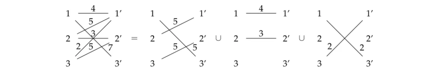
1 1’ 2 2’ 3 3’ 4 7 5 3 2 5 = 1 1’ 2 2’ 3 3’ 5 5 5 ∪ 1 1’ 2 2’ 3 3’ 4 3 ∪ 1 1’ 2 2’ 3 3’ 2 2
Figure 2.Valid schedule (step 1 as a duration of 5, step 2 a duration of 4 and step 3 a duration of 2). If β = 1 the total cost of the schedule is 3+11=14. Note that, thanks to the preemption the communication of duration 7 is decomposed of a communication of duration 5 and a communication of duration 2
suppose that this network can handle at most k communications at the same time between the two clusters. For instance if both clusters have 100 Mbit network cards and are interconnected by a 1 Gbit network there can be at most k = 10 communications at the same time without contention. We suppose that k is smaller than the number of nodes of both clusters. In this case when a cluster must redistribute its data from all its nodes to all the nodes of the other cluster it is required to schedule the communication in order to avoid contention.
The considered application is composed of computing phases and communication phases than can overlap. When a communication phase consists in transmitting data from one cluster to the other (no local communica-tions) it is called a redistribution phase.
Each redistribution phase is considered separately. A redistribution phase is modeled by a redistribution
ma-trix M = mi,jwhere mi,jis the time for sending the data from node i of the first cluster to node j of the second
one. This time is computed by dividing the amount of data to be sent by the speed of the communication when no contention occurs. We suppose that this matrix is given and computed by an other module of the application. The redistribution is performed by steps. In order to optimize the solution we allow preemption. This means that at the end of a step, communication can be stopped and resumed in an other step.
We denote by β the time to setup a communication step (it takes into account the time to open the sockets, the latency of the network, the preemption etc.).
Finally we do not allow contention on the network card. This means that we work in the 1-port model. During one step, a node can receive (resp. send) at most one communication from (resp. to) an other node.
2.2
Formulation
We provide here a graph formulation for the redistribution problem. It is called KPBS for K-Preemptive
Bipar-tite Scheduling. A matrix can be seen as a biparBipar-tite graph. Let M = mi,j a redistribution matrix with n1 lines
and n2columns (this means that the first cluster has n1nodes while the second cluster has n2nodes). We build a
bipartite graph with n1vertices on one side and n2vertices on the other. We draw an edge from node i of the first
side to node j of the second side if element mi,jof M is not zero. We label this edge by mi,j(see Figure 1 for an
example).
A step S is modelized by a bipartite graph too. In order for this step to be valid it has to model at most k communications and no node can perform more than one communication (1-port model). This means that the bipartite graph has to be a matching with at most k edges. The duration of a step is the startup time plus the
duration of its longest communication (m = max(si,j)) where si,jis the duration of the communication between
node i and node j for this step.
A valid schedule of the redistribution is a set of s valid steps Sisuch that M = ∪si=1Si. The cost of the schedule
is the sum of the cost of each step :Ps
i=1(β + mi), where miis the length of step i (see Figure 2).
2.3
Related works
The KPBS problem generalizes several well known-problem of the literature:
• The problem of redistributing data inside a cluster has been studied in the field of parallel computing for years [7, 17]. In this case the modelization and the formulation is the same except that the number of
messages that can be send during one step is only bounded by the number of nodes (k = min(n1, n2)).
• The problem has been partially studied in the context of Satellite-Switched Time-Division Multiple Access systems (SS/TDMA) [3, 11, 12]. The problem with β = 0 is studied in [3]. Finding the minimum number of steps is given in [11].The problem when no preemption is allowed is studied in [12].
• Packet switching in communication systems for optical network problem also called wavelength-division multiplexed (WDM) broadcast falls in KPBS [4, 8, 16, 18, 11]. In [8, 11], minimizing the number of steps is
studied. In [4] and in [16], a special case the KPBS problem is studied when k = n2
The problem of finding an optimal valid schedule has been shown NP-complete in [5].
In [14] we have proposed two 2-approximations schedule algorithms (the found schedule is never twice as long as the optimal one) for KPBS. These algorithms are called GGP (Generic Graph Peeling) and OGGP (Optimized GGP). It is out of the scope of this report to describe them in details (see [5, 14] for more information).
2.4
Other Notations
We note
• G = (V1, V2, E, w)the bipartite graph, with V1and V2the sets of senders and receivers, E the set of edges,
and w the edges weight function,
• P (G) =Pe∈Ew(e),
• W (G) = maxs∈V1∪V2(w(s))with w(s) the sum of the weigths of all edges adjacent to s,
• ηo: the estimated redistribution time for when no scheduling is performed.
3 Predicting redistribution time
We present here how we predict the redistribution time. Two approaches are studied. One, called thebrute-force
approach, is used when no scheduling is performed at the application level and when the transport layer manage the contention by itself. In this case all the messages are sent at the same time. In the other approach, called the
scheduling approach we use (O)GGP to schedule the messages and the contention is managed at the application
level.
3.1
Brute-force approach
As the time needed by (O)GGP to compute and issue a schedule of all communications is not negligible, it is useful to develop a quick algorithm to estimate the time needed by the brute force approach. This could enable a quick decision algorithm as whether or not use a scheduling approach.
We assume that the application is running on a dedicated platform. Therefore, we assume no random pertur-bation on the network. In our modelization, we do not take into consideration the cost of network congestion. Estimating the significance of packet losses is of interest, but requires a different approach, less precise, which should be studied apart.
Therefore, the proposed algorithm gives an estimation of the optimal redistribution time achievable using a brute force approach on a perfect network.
We call ηothe estimated redistribution time of the brute-force approach.
In the remaining, edge of redistribution pattern (Figures 3, 4, 6, 7, 8), are labeled are in seconds. This means that when no contention occurs it requires the given time to transfer the data between the nodes. If more than k communications occur at the same time the network is assumed to be fairly shared.
Lower bound-based prediction
Several possibilities present themselves for computing ηo. The easiest method is to take the maximal time
between P(G)
k and W (G). In other words ηodepends either from the bottleneck generated by the bandwidth of
the network, or from the bottleneck generated on a local link by the sender or the receiver who has the most data
to send. While this gives a lower bound of ηo, quick to compute, we can show that such an estimation of ηois not
always accurate. For example consider the graph of Figure 3.
With k = 2 we can see that P(G)
k = 4
2 = 2and W (G) = 2. So we know it needs at least 2 seconds to issue the
redistribution.
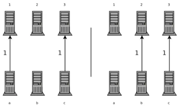
Figure 3. Simple redistribution pattern withk= 2
However the brute force redistribution takes place in two steps: At first, every node is sending data. As we
assume that the network is fairly shared, the speed of the 3 communications is slowed-down by a factor of 3
k.
Therefore It takes 1 ×3
2 = 1.5seconds to send the data between nodes 1 and a and 2 and b because k = 2. After
that time there is only one communication remaining (between node c and node 3). It takes 1 second to send the data remaining between these nodes. Therefore, the total time taken by the brute force redistribution is here of
2.5seconds, that is 25% higher than the estimation.
This shows there is a need for a more precise way to compute ηo. We can also see that the scheduled
redistribu-tion of Figure 4 takes 2 second to execute, reaching the optimal time (without taking into account the time needed to establish the communications).
Figure 4. Schedule of the pattern of Fig. 3 in two steps
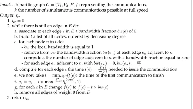
Input: a bipartite graph G = (V1, V2, E, f)representing the communications,
kthe number of simultaneous communications possible at full speed
Output: ηo
1. ηo= 0
2. while there is still an edge in E do:
a. associate to each edge e in E a bandwidth fraction bw(e) of 0 b. build l a list of all nodes, ordered by decreasing degree c. for each node n in l do:
- bw the local bandwidth is equal to 1
- remove from bw the bandwidth fraction bw(en)of each edge enadjacent to n
- compute a the number of edges adjacent to n with a bandwidth fraction equal to zero
- for each edge enadjacent to n, with bw(en) = 0, bw(en) = bwa
d. compute for each edge e the time t(e) = f(e)
bw(e) needed to issue the communication
e. we now take t = mine∈E(t(e))the time of the first communication to finish
f. ηo= ηo+ t ×max(
P
e∈Ebw(e) k ,1)
g. for each e in E change f(e) to f(e) − t × bw(e) h. remove all edges of weight 0 from E
3. return ηo
Figure 5.Estimation Algorithm
Prediction algorithm
Computing ηois done using the algorithm of Figure 5. It is a discrete event simulation of the redistribution. The
principle is the following : as the fraction of bandwidth available for an edge only depends on the redistribution pattern, we compute the fraction of bandwidth available for each communication. We then compute the time needed to finish each communication. We take the first communication to finish, remove it from the graph and add its time to the total time needed. At this point the redistribution pattern changed, so the amount of bandwidth available for everyone changes and we need to start again the algorithm. A formal description of the algorithm is given in Figure 5.
We should note that the bandwidth fraction associated with each edge is always between 0 and 1. It cannot be greater than 1 since (at step 2.c) bw has an initial value of 1 which can only be decreased or divided. An allocated bandwidth fraction cannot be higher than 1 divided by the degree of the node already treated by the algorithm.
Since the nodes are treated in decreasing degree order, it cannot be greater than 1
degree(n). Therefore the sum
of all bandwidths bw(en)computed at step 2.c cannot be greater than degree(n) ×degree1
(n) = 1. And hence, a
bandwidth fraction cannot be lower than 0.
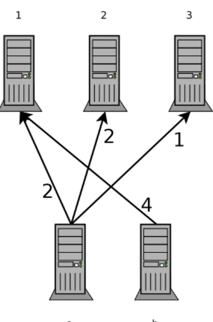
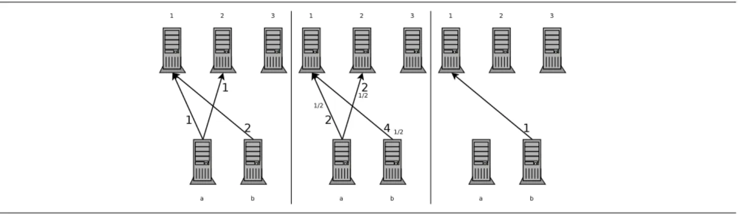
We start with node a which is of degree 3, the highest one. All 3 edges connected to a have no bandwidth fraction already allocated. Therefore, we split the available bandwidth in 3. Each of these edges now has a
bandwidth fraction of 1
3. The next node is node 1, with a degree of 2. We compute the bandwidth fraction left
for this node, which is 1 − 1
3 = 2
3 (edge (a,1) already use one third of it). Only one edge, between 1 and b,
has no bandwidth allocated: it receives the whole bandwidth fraction left (2
3). At this point, all edges have a
bandwidth fraction assigned: We have finished substep c of the algorithm. We now compute for each edge the
communication time needed at this speed. For example the communication between 1 and b takes 4
2 3
= 6seconds.
The results of all these computations are displayed in Figure 7, the time being displayed in bold.
The shortest time is for the communication between node 3 and node a, so we are going to issue 3 seconds of
communications. For example the edge between 1 and b has its weight reduced by 3 × 2
3 = 2. ηois now 3, as the
network can handle a bandwidth of 3 (k = 3) and the sum of all bandwidths is 3 ×1
3+ 2 3 =
5
3 < k. Only the edge
Figure 6. Initial pattern
Figure 7. Bandwidth fraction and time
between 3 and a has now a weight of 0: it is the only to be removed from G. We repeat the algorithm at step a. The remaining computations are shown in Figure 8. You can notice that it is perfectly possible to finish several communications in one step.
Figure 8.Other steps of computations
The total time for ηois here 6 seconds, whereas the optimal time is 5 seconds (β = 0).
In this small example, we can see that the termination of the communication between a and 3 change the bandwidth available for every other communications.
On large graphs, with more edges, it is possible to find this behavior of one communication modifying the entire state of all others. On low latency networks, TCP is able to adapt itself quickly, however should the latency increase, the time needed to adjust all bandwidths for each flow could raise and hinder performances.
3.2
Scheduling approach
Estimating the time needed for a schedule redistribution is straightforward. We compute the cost of the sched-ule as described in section 2.2.
4 Experiments
We conducted several experiments to test the efficiency and the validity of our estimations.
4.1
Simulation
We showed in the previous section that in some cases, a simple redistribution could give worse results than a scheduled one, even with low network constraints. However this effect is strongly dependent from the input redistribution pattern and it can be asked if this really reflects the behavior of real-life programs.
Marc Grunberg, Stéphane Genaud and Catherine Mongenet did in [13] some geophysics experiments on differ-ent platforms including a grid platform. The experimdiffer-ents are mainly divided in two parts, a computation phase, and a final redistribution phase taking on the grid platform an important amount of time.
With access to the log files of the experiments, we extracted the redistribution pattern, and constructed the
corresponding bipartite graph. We then computed ηoand the time of the scheduled redistribution for different
values of k. The results are shown in Figure 9 with k on the abscissa and on the ordinate the amount of time gained using a scheduling over a brute force approach. We clearly see that it is perfectly possible to achieve up to 20% enhancements on this particular application.
4.2
LAN experiments
In order to prove both the accuracy of the evaluation of ηoand the existence of redistribution patterns giving a
suboptimal performance we conducted experiments on a real local area network.
0 5 10 15 20 25 1 2 3 4 5 6 7 8 gain k results tcp vs GGP comparison
Figure 9. Comparison of schedule time andηo
The platform running the tests is composed of two clusters of 10 1.5Ghz PC running Linux and interconnected by two switches. All links, switches and Ethernet adapters have a speed of 100Mbits. With such a configuration, only one communication is needed to saturate the network of the network and thus k = 1. In order to test interesting cases, that is where k 6= 1, we limited the available incoming and outgoing bandwidth of each network
card to100
k Mbits per second. This was done using thershaper [19] Linux kernel module. This module implements
a software token bucket filter thus enabling a good control of the available bandwidth. Standard linux QOS
modules (sch_ingress, sch_tbf ) have also been tested and giving the same results. We conducted experiments for
k= 5. All tests were conducted without interferences from other network users.
All communications routines have been implemented by hand using standard POSIX sockets and threads to get maximal performance and a complete control over communications.
We implemented a brute force redistribution algorithm. All communications are issued simultaneously, and the TCP is handling the network congestion. We also implemented a scheduled redistribution algorithm consist-ing of several redistribution steps synchronized usconsist-ing barriers. The scheduled has been obtained usconsist-ing our GGP algorithm [14].
The first tests are executed on some random redistribution patterns. The input data always has the same num-ber of communications, however of random weights, and between random senders and receivers. The weights are generated uniformly between 10MB and xMB. All further plots are obtained as x increases from 10MB to 80MB. The first estimation for the brute force time is done computing the lower bound of the communication time and the second one using the algorithm of Figure 5. We executed the redistribution and computed the accuracy of the two estimations as the size of the data increases. We also compared the time estimated for the scheduled redistri-bution with the real time obtained. We can see in Figure 10 that all methods are giving a reasonable estimation of
the real redistribution time, with ηobeing slightly more precise for the brute force redistribution.
92 94 96 98 100 102 104 106 10 20 30 40 50 60 70 80 90 100 accuracy data size (MB) efficiency of time approximation
eta opt bound scheduled estimation
Figure 10. Accuracy ofηoevaluation
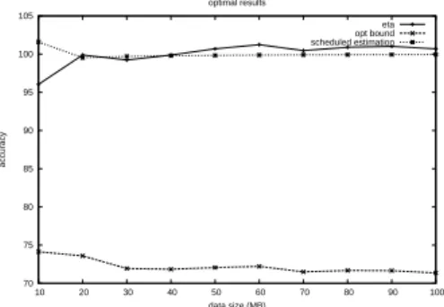
We then tested the redistribution on the kind of redistribution pattern yielding theoretically to worse brute force results described in Section 2. Again, we computed the accuracy of the time estimations as the size of the
input data grows. The results displayed in Figure 11 show that the experiments confirm the theory. The optimal
time is far under the real time observed, whereas the ηoestimation is close from it. Again, the time computed for
the scheduled reditribution is close from the real time observed.
70 75 80 85 90 95 100 105 10 20 30 40 50 60 70 80 90 100 accuracy data size (MB) optimal results eta opt bound scheduled estimation
Figure 11. Accuracy ofηoevaluation
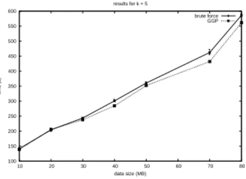
Finally we compared the efficiency of (O)GGP over a brute force redistribution: Several redistribution patterns have been used:
At first we used some random graphs. Figure 13, Figure ?? and Figure 14 show the time obtained for graphs of 25,35 and respectively 45 edges as the maximal data size increases.
50 100 150 200 250 300 10 20 30 40 50 60 70 80 time (s) data size (MB) results for k = 5 brute force GGP
Figure 12. Times obtained on random graphs of 25 edges
100 150 200 250 300 350 400 450 20 30 40 50 60 70 80 time (s) data size (MB) results for k = 5 brute force GGP
Figure 13. Times obtained on random graphs of 35 edges
We can see that the scheduled redistribution is performing better than the brute-force redistribution with some peaks of 7% improvements. The results are better for larger graphs (we believe this is due to an increased variation in the edges weight).
100 150 200 250 300 350 400 450 500 550 600 10 20 30 40 50 60 70 80 time (s) data size (MB) results for k = 5 brute force GGP
Figure 14. Times obtained on random graphs of 45 edges
We also tried as input the family of graphs giving theoretically bad performances with the brute-force redistri-bution. The results shown in Figure 15 confirm again the theory. The scheduled redistribution is on average 30% faster than the brute force redistribution. We can also see that as the redistribution pattern is kept the same with only increasing weights, the times scale linearly with the data size.
0 20 40 60 80 100 120 140 10 20 30 40 50 60 70 80 90 100 time (s) data size (MB) optimal results brute force GGP
Figure 15. Comparison of schedule time and raw time
5 Conclusion
Data redistribution is a critical phase for many distributed-cluster computing applications such as code cou-pling or computational steering ones. Scheduling the messages that have to be transmitted between the nodes can be performed by the transport layer of the network (TCP) or by the application (using the knowledge of the redistribution pattern).
In this report we have studied the redistribution phase in the context of a low latency network (LLN), such as LAN. In this case, the reactivity of TCP is nearly perfect and the transport layer should give very good perfor-mance. This is the worst-case scenario for application level scheduling algorithm.
We have provided a modelization of the behavior of TCP for the data redistribution problem as well as of scheduling algorithms proposed in early works and called GGP and OGGP. We have compared two ways of predicting the data redistribution time. One is based on an inferior bound easily derived from the redistribution pattern, the other is based on the analysis of the pattern and our modelization of the platform. Whereas the first way is shown to be accurate only for certain redistribution pattern, the second approach gives very accurate predictions for any redistribution pattern. Whatever the scheduling is performed at, the application level or the transport level, we are able to predict accurately the redistribution time.
We have experimentally compared the performance of (O)GGP against the brute-force approach that consist in let the transport layer manage the congestion alone on LLN. Suprisingly, results show that even if the reactivity of transport-layer is nearly perfect, (O)GGP always outperform the brute-force approach (up to 30%).
Future works are directed towards the study of fully heterogeneous platforms where the network cards of each node can have different speed. This removes the 1-port constraint assumption, and modifies our modelization.
Bibliography
References
[1] F. Afrati, T. Aslanidis, E. Bampis, and I. Milis. Scheduling in switching networks with set-up delays. In
AlgoTel 2002, Mèze, France, May 2002.
[2] P.B. Bhat, V.K. Prasanna, and C.S. Raghavendra. Block Cyclic Redistribution over Heterogeneous Networks. In11thInt. Conf. on Parallel and Distributed Computing Systems (PDCS 1998), 1998.
[3] G. Bongiovanni, D. Coppersmith, and C. K. Wong. An Optimum Time Slot Assignment Algorithm for an
SS/TDMA System with Variable Number of Transponders. IEEE Transactions on Communications, 29(5):721–
726, 1981.
[4] H. Choi, H.-A. Choi, and M. Azizoglu. Efficient Scheduling of Transmissions in Optical Broadcast Networks.
IEEE/ACM Transaction on Networking, 4(6):913–920, December 1996.
[5] Johanne Cohen, Emmanuel Jeannot, and Nicolas Padoy. Messages Scheduling for Data Redistribution
be-tween Clusters. InAlgorithms, models and tools for parallel computing on heterogeneous networks (HeteroPar’03)
workshop of SIAM PPAM 2003, LNCS 3019, pages 896–906, Czestochowa, Poland, September 2003.
[6] P. Crescenzi, D. Xiaotie, and C. H. Papadimitriou. On Approximating a Scheduling Problem. Journal of
Combinatorial Optimization, 5:287–297, 2001.
[7] F. Desprez, J. Dongarra, A. Petitet, C. Randriamaro, and Y. Robert. Scheduling Block-Cyclic Array
Redistri-bution. IEEE Transaction on Parallel and Distributed Systems, 9(2):192–205, 1998.
[8] A. Ganz and Y. Gao. A Time-Wavelength Assignment Algorithm for WDM Star Network. InIEEE
INFO-COM’92, pages 2144–2150, 1992.
[9] G.A. Geist, J.A. Kohl, and P.M. Papadopoulos. CUMULVS: Providing Fault-Tolerance, Visualization and
Steering of Parallel Applications. International Journal of High Performance Computing Applications, 11(3):224–
236, August 1997.
[10] A. Goldman, D. Trystram, and J. Peters. Exchange of Messages of Different Sizes. In Solving Irregularly
Structured Parblems in Parallel, number 1457 in LNCS, pages 194 – 205. Springer Verlag, August 1998.
[11] I.S. Gopal, G. Bongiovanni, M.A. Bonuccelli, D.T. Tang, and C.K. Wong. An Optimal Switching Algorithm
for Multibean Satellite Systems with Variable Bandwidth Beams.IEEE Transactions on Communications,
COM-30(11):2475–2481, November 1982.
[12] I.S. Gopal and C.K. Wong. Minimizing the number of switching in an ss/tdma system. IEEE Trans. on
Communications, 33:497–501, 1885.
[13] Marc Grunberg, Stephane Genaud, and Catherine Mongenet. Seismic ray-tracing and Earth mesh modeling
on various parallel architectures. The Journal of Supercomputing, 29(1):27–44, July 2004.
[14] E. Jeannot and F. Wagner. Two Fast and Efficient Message Scheduling Algorithms for Data Redistribution
through a Backbone. In18th International Parallel and Distributed Processing Symposium, page 3, April 2004.
[15] K. Keahey, P. Fasel, and S. Mniszewski. PAWS: Collective Interactions and Data Transfers. In10th IEEE Intl.
Symp. on High Perf. Dist. Comp. (HPDC-10’01), pages 47–54, August 2001.
[16] G.R. Pieris and Sasaki G.H. Scheduling Transmission in WDM Broadcast-and-Select Networks. IEEE/ACM Transaction on Networking, 2(2), April 1994.
[17] L. Prylli and B Tourancheau. Efficient Block-Cyclic Data Redistribution. InEuropar’96, LNCS 1123, pages
155–164, 1996.
[18] N. Rouskas and V. Sivaraman. On the Design of Optimal TDM Schedules for Broadcast WDM Networks
with Arbitrary Transceiver Tuning Latencies. InIEEE INFOCOM’96, pages 1217–1224, 1996.
[19] A. Rubini. Linux module for network shaping
http://ar.linux.it/software/.
Unité de recherche INRIA Lorraine
LORIA, Technopôle de Nancy-Brabois - Campus scientifique
615, rue du Jardin Botanique - BP 101 - 54602 Villers-lès-Nancy Cedex (France)
Unité de recherche INRIA Rennes : IRISA, Campus universitaire de Beaulieu - 35042 Rennes Cedex (France) Unité de recherche INRIA Rhône-Alpes : 655, avenue de l’Europe - 38330 Montbonnot-St-Martin (France) Unité de recherche INRIA Rocquencourt : Domaine de Voluceau - Rocquencourt - BP 105 - 78153 Le Chesnay Cedex (France)
Unité de recherche INRIA Sophia Antipolis : 2004, route des Lucioles - BP 93 - 06902 Sophia Antipolis Cedex (France)
Éditeur
INRIA - Domaine de Voluceau - Rocquencourt, BP 105 - 78153 Le Chesnay Cedex (France)
http://www.inria.fr