ANALYSING FLUX DECLINE IN DEAD-END FILTRATION

HAL Id: hal-00329472

https://hal.archives-ouvertes.fr/hal-00329472

HAL is a multi-disciplinary open access archive for the deposit and dissemination of sci-entific research documents, whether they are pub-lished or not. The documents may come from teaching and research institutions in France or abroad, or from public or private research centers.

L’archive ouverte pluridisciplinaire HAL, est destinée au dépôt et à la diffusion de documents scientifiques de niveau recherche, publiés ou non, émanant des établissements d’enseignement et de recherche français ou étrangers, des laboratoires publics ou privés.

ANALYSING FLUX DECLINE IN DEAD-END

FILTRATION

Alexia Grenier, Martine Meireles, Pierre Aimar, Philippe Carvin

To cite this version:

Alexia Grenier, Martine Meireles, Pierre Aimar, Philippe Carvin. ANALYSING FLUX DECLINE IN DEAD-END FILTRATION. Chemical Engineering Research and Design, Elsevier, 2008, 86, pp.1281-1293. �10.1016/j.cherd.2008.06.005�. �hal-00329472�

ANALYSING FLUX DECLINE IN DEAD-END FILTRATION

1 2

Alexia Grenier, Martine Meireles1, Pierre Aimar, Philippe Carvin2 3

4

Université de Toulouse 5

Laboratoire de Génie Chimique, UMR CNRS 5503 6

Université Paul Sabatier 7

118 route de Narbonne 8

31062 Toulouse Cedex 9, France 9

10 11

Abstract

12

Can we rely on the analysis of flux decline to evaluate the risks of a filter media to be clogged 13

during filtration of a given particle suspension? This important issue can be dealt with a 14

macroscopic approach described in this paper. We seek to identify and quantify the successive 15

prevailing mechanisms which occur during a filtration run, directly and solely from 16

experimental flux data. This is achieved from the collection of experimental data (filtrate 17

volume V versus time t) and the use of the differential equation

2 2 n d t dt k dV dV ⎛ ⎞ = ⋅⎜ ⎟ ⎝ ⎠ . A 18

methodology is then proposed to define and validate experimental procedures with the 19

purpose of quantifying occurring fouling mechanism. For the purpose of illustrating its 20

valuable impact for a bench marking procedure, the methodology has been applied on a 21

model system composed of a bentonite suspension and a series of microfiltration membranes 22

of different structures. 23

24

Keywords: Microfiltration, Flux decline, Blocking, Fouling mechanisms, Filter media

25 26

1 _{Corresponding author : meireles@chimie.ups-tlse.fr}

1. Introduction

1 2

Microfiltration is a separation process by which some constituents of a suspension are 3

separated from the liquid by a membrane mainly acting as a sieve. Ideally the membrane 4

allows the passage of the fluid through its pores while retaining all suspended solid particles 5

originally present in the fluid. The ideal picture stands if solid particles are all larger than the 6

pores of the membrane and the pore structure consists in capillaries. However in almost all 7

practical cases a fairly wide range of effective particle sizes exists in the feed as well as a 8

random distribution of pores exists in the membrane. In usual cases, when filtering 9

suspensions containing more than a few percents of solids, blocking of particles inside or on 10

the top of the membrane occurs, leading to a reduction in filtration flux. There are four 11

mechanistic models that are generally used to describe fouling 1,2 . . 12

• Complete blocking assumes a seal of pore entrances and the prevention of any flow 13

through them. As pore entrances are sealed, the area open to flow is reduced. 14

• Intermediate blocking also assumes a seal of pore entrances by a fraction of particles 15

and a deposition of the rest on the top of them. 16

• Cake filtration is a mechanism by which particles accumulate at the surface in a 17

permeable cake of increasing thickness that adds a hydraulic resistance to filtration. 18

• Finally standard blocking assumes an accumulation inside the membrane on the pore 19

walls. As the pores are constricted, the membrane permeability is reduced. The 20

mathematical expressions for these laws are summarized in Table 1. These 21

expressions were derived by Hermans and Bredée 3, on the assumption of separate 22

mechanisms. All these different laws stem from a common differential equation. For a 23

constant pressure filtration they have been reformulated in a common frame of power-1 law relationships4: 2 n dV dt k dV t d ⎟ ⎠ ⎞ ⎜ ⎝ ⎛ = 2 2 (1) 3

Table 1 presents the physical basis for each fouling mechanism and the corresponding n-value 4

according to Eq. (1). The blocking filtration laws have also been extensively used under their 5

linear form detailed in Table 4. 6 Table 1: 7 Fouling mechanism n Corresponding linear

form Physical concept

Cake Filtration 0

( )

( )

Pore blocking + surface deposit Standard Blocking 1.5

( )

( )

Each of these mechanisms has been individually invoked alone or in combinations, to explain 9

experimental observations. Most of the time the model which best fits the experimental data is 10

claimed to capture the fouling mechanism. 11

For filtration of BSA proteins suspensions, standard blocking, intermediate blocking or 12

complete blocking models were found to fit the experimental data 5 with the intermediate 13

model providing the best fit. A combination of standard or complete model and subsequently 14

cake model was also found to fit the data well for the same system 6_{. In some other}

15

conditions, 7, it was observed that fouling of microfiltration membranes by BSA did not 16

follow any of the individual models and is more likely described by a combination of several 17

models. These results show that the predominant mechanisms may vary with operating 1

conditions. 2

Recently a model has been proposed based on a combination of blocking laws in a two-stage 3

mechanism 8. Fouling initially occurred through complete blocking and subsequently through 4

cake formation. The deposited assemblages were assumed to be permeable so that the flow 5

through the blocked areas also participate to cake formation. The authors found this model 6

provided good data fits for the fouling of microporous track-etched membranes by five 7

proteins. The previous model was further expanded by using a method to combine the four 8

individual blocking laws 9 The combined models (cake filtration- complete blocking model, 9

cake filtration-standard blocking model) were assessed by testing solutions of bovine serum 10

albumin and human IgG under constant pressure and constant flow modes. The combined 11

cake-complete blocking model provides good fits of both data sets. 12

Combined best fitted models allow a better determination of the membrane capacity, defined 13

as the amount of fluid per membrane are which can be processed until the flux declines to a 14

preset fraction of the initial flux or until the caking starts leading to a several-fold increase in 15

the filtration resistance. 16

Combination of mechanisms has been also been reported for filtration of particles 17

suspensions. For example, the analysis of experimental flux decline during filtration of size 18

distributed carbonyl iron suspensions through woven filter media shows that fouling is 19

initially controlled by standard blocking mechanism prolonged by a cake filtration period 1_.

20

Owing to the impact of porous structure clogging on the lifetime of the filter media, the 21

characterization of the mechanism occurring in the initial period may largely serve to choose 22

the appropriate filter media. An important difficulty lies in the determination at lab scale of 23

this critical initial period. Dilution which extends its duration can be a way but the question 24

may be raised if the same mechanisms occur as for higher solid concentrations. 25

1

This works intends to complete previous studies by setting a methodology to analyse 2

experimental flux decline for dead-end filtration runs and identify successive prevailing 3

mechanisms As developed further on, we shall simply assume three types of blocking 4

mechanisms (cake, complete blocking and standard fouling) The methodology can be 5

implemented even in the absence of precise information on the “suspension” or on the filter 6

(for instance, particle size distribution, mean particle diameter, pore size distribution, nominal 7

pore diameter, zeta potential, etc.) and is applicable to various systems (in this paper, we 8

report the results obtained with a bentonite suspension filtered through four microfiltration 9

membranes of different pore size). 10

In our approach, we made the choice of not to describe the transitions between two apparent 11

fouling regimes when two different mechanisms may compete, a point of view which differs 12

from other work 8, but to approximate the filtration curve into several successive apparent 13

steps during which only one fouling mechanism is predominant. We also made the choice not 14

to dilute the feeds but to develop an appropriate data analysis to capture the initial regime of 15

blocking. 16

In this paper, the main steps of the approach are detailed. Then we see how one could select a 17

filter medium adapted to the filtration of a given suspension and we present how the blocking 18

coefficients deduced with our methodology evolve when parameters such as feed suspension 19

concentration, transmembrane pressure or mean pore diameter change. 20

21

2. Modelling flux decline

22

The approach proposed is based on the flux decline analysis. Three types of fouling 23

mechanisms have been considered (cake, complete blocking and standard blocking) leading to 24

a flux decline. Each mechanism is denoted by a specific subscript as : 25

- (B) for complete blocking defined as particle capture at the ‘suspension - filter’ interface; 1

- (C) for cake formation defined as particle capture at the top surface of the filter (to form a 2

cake or a deposit); 3

- (I) for standard blocking defined as particle capture inside the filter. 4

5

A series description for the different mechanisms

6

The evolution of the permeate flux, J, with filtration time has been modelled by a classical 7 Darcy law 10: 8 R P J ⋅ Δ = μ (2) 9

where R is a hydraulic resistance. 10

Accordingly , the permeate flux is expressed by: 11

(

)

where Rm and RC correspond to the hydraulic resistances of the filter (fouled or not) and the

13

hydraulic resistance of the cake, respectively. As in an unstirred system, we use the classical 14

assumption that the deposit is covering the entire area of the filter. 15

Complete Blocking (B)

16

Concerning the complete blocking mechanism, we use a surface coverage ratio, βB,8.to

17

characterize the surface fraction open to the flow. This ratio may evolve during a certain time 18

and then remains constant when complete blocking is not prevailing anymore. The surface 19

coverage ratio βB increases with the cumulative permeate volume, V, at a rate characterised by

20

the blocking parameter ηB:

J dt d B B =η × β (4) 1

Equation (4) can also be reformulated as : 2 0 A V B B =η × β (5) 3

ηB is the blocked surface area by unit of time and surface of the membrane ( see Appendix I)

4

When a surface blocking prevails, the filter hydraulic resistance, Rm,B, is directly a function of

5 βB according to : 6 ,0 , 1 m m B B R R β = − (6) 7 also reformulated as : 8 0 0 , , 1 A V R R B m B m × − = η (7) 9 0 , m

R is the clean membrane hydraulic resistance. It can be calculated from permeability tests

10

on the clean ( non fouled) membrane before any filtration experiment. 11

Cake Formation (C)

12

The cake hydraulic resistance, RC, increases with the cumulative permeate volume V, at a rate

13

characterised by ηC for cake formation (C) according to the following equation:

14 V A R C C = × 0 η (8) 15

ηC is the volumic specific resistance of the cake ( see Appendix I).

Internal Fouling (I)

1

The filter resistance, Rm,I, increases with the cumulative permeate volume V, at a rate

2

characterised by ηI for internal fouling (I), according to the standard blocking law:

3

(

)

ηI is the volume of particle accumulated in the media per unit of permeate volume and per

5

unit of void volume. 6 7 3. Materials 8 9 3.1. Suspension 10 11

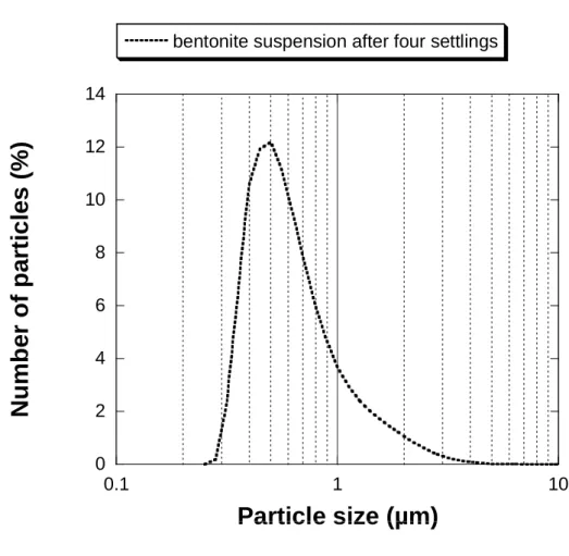
Bentonite (clay) particles are platelets; the larger dimension of these platelets of about 1 12

micrometer is about one hundred times the thickness (showing a large shape factor). Their 13

basal face is positively charged, whereas the particle edge is negatively charged. 14

A first suspension was prepared by dispersing 30 g of clay powder in 1 litre of deionised 15

water. Four settlings (each 4-hour long) lead to a stock suspension of 19 g.L-1consisting of 16

micron sized particles. This suspension exhibits a broad particle size distribution around 0.5 17

µm (see Figure 1) determined by dynamic light scattering experiments (Mastersizer 2000, 18

Malvern Instruments). Suspensions in the concentration range 10-3 g.L-1 to 10 g.L-1 are 19

prepared by dilution of the stock solution with deionised water. 20

21

3.2. Filter media

22 23

Four microfiltration membranes have been tested with different nominal pore sizes as 1

provided by manufacturers (0.2, 0.8, 5 and 8 µm). The 0.2 and 0.8 µm membranes are made 2

of cellulose acetate (Schleicher & Schuell). The 5 and 8 µm membranes are made of mixed 3

cellulose esters (Millipore). According to information provided by manufacturers, nominal 4

pore sizes are measured by liquid displacement methods 5

6

3.3. Experimental set-up

7 8

The filtration system is composed of an air-pressurized feed tank connected to a 50-mL 9

filtration cell (Millipore). A fresh membrane is mounted up in the filtration cell and the 10

reservoir is first filled with deionised water. The system is pressurised until a steady state flux 11

is obtained. The cell is then emptied and refilled with the suspension to be filtered. Filtration 12

experiments are conducted at different pressures and different concentrations of suspension 13

without any stirring of the suspension. The permeate is collected in a beaker and the 14

cumulative permeate mass is measured via an electronic balance connected to a computer for 15

on-line data acquisition. At the end of the filtration run, the used microfiltration membrane is 16

discarded and the filtration cell is emptied. For a given set of operating conditions ( feed 17

concentration, transmembrane pressure), the permeate versus volume data are collected from 18

a series of five runs. 19

20

4. Methodology background

21 22

The first objective is to identify which fouling mechanisms are prevailing and when, 23

during a filtration experiment. Even if we do know that fouling phenomena can 24

simultaneously occur, we assume that a filtration run can be split into several successive steps 25

in which only one fouling mechanism is prevailing. Flux decline analysis requires a rigorous 1

procedure so as to discriminate between the different fouling mechanisms from a 2

differentiation of experimental data such as in equation (1). 3

From a filtration data set, V t

( )

4

method in order to derive parameters from the ⎟

⎠ ⎞ ⎜ ⎝ ⎛ = dV dt f dV t d 2 2 equations. In order to 5

attenuate the noise in experimental data, a smoothing method is used: the moving average 6

filtering method. It is a low pass filter that averages five neighbouring data. This method

7

proved to be simple and efficient. Lastly, the finite differences method11 is used to 8

numerically derive V t

( )

2 dV t d and dVdt . 9 10

Prevailing fouling mechanisms

11

In Table 1, it has been noticed that a specific value of n characterizes each given fouling 12

mechanism. In the cases for which the value of n found experimentally is different from the 13

ones given in Table 1, we do not have any physical fouling model that corresponds to the flux 14

decline: there may be a combination of several identified or not identified mechanisms. 15

16

Let us now focus on the exponent n. The value of n enables the identification of the 17

controlling fouling mechanisms, whereas the determination of k permits the quantification of 18

the identified fouling mechanism.(see Table 2). 19 20 Table 2 21 Fouling mechanisms k n Cake Filtration P A C Δ ⋅ ⋅ 0 η μ 0

Standard Blocking _{2. .} 1/2 o I Q η 1.5 Complete Blocking B A Q _η ⋅ 0 0 2 1

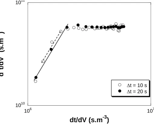
According to Figure 2 and Table 3, when k is derived by fitting equation (1) to experimental 2

data, it is greatly influenced by the time step Δt used in the differentiating method.

3 4 Table 3 5 Time step (Δt) k n 10 s 1.4 × 10-2 _2.0 20 s 3.7 × 10-2 _1.9 6

Accordingly, it seems more appropriate to use Equation (1) for mechanism identification 7

purposes only (evaluation of n) but not for quantification (estimation of k). k will therefore be 8

determined by using the linear form of the models (Table 1). 9

Besides, the use of equation (1) also allows the determination of a range of specific data for 10

which a given mechanism is controlling the flux decline process. The blocking parameters are 11

then evaluated on the data range corresponding to a period of time where the blocking law 12

prevails, which is a key point of this methodology. 13

14

Determination of blocking parameters

15

Once the data range has been determined for each fouling mechanism, the parameters can be 16

evaluated from the plot of the linear form of the considered fouling mechanism (Table 4). 17

18

Table 4: 19

mechanism Cake Formation _dVdt = f

( )

(

)

(

)

( )

(

)

( )

Approximation of the filtration in several successive fouling regimes

2

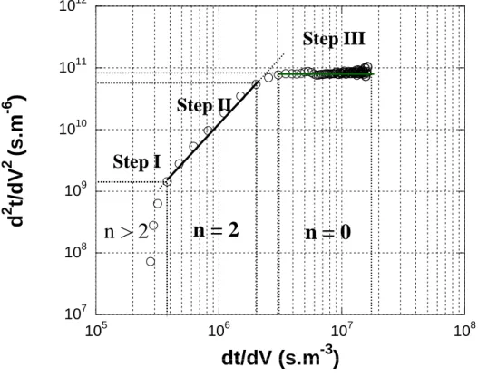
As for an example, for the ‘bentonite-.5 μm membrane’ system (Figure 3), this method allows 3

to identify two fouling regimes 4

- A very low fouling (VLF) regime, in our description the flow rate is indeed assumed to 5

remain constant . We use the average value over the time period (Step I). This 6

duration is actually an approximation since the permeate flow rate slightly decreases 7

during this period (Figure 4). But according to the ⎟

⎠ ⎞ ⎜ ⎝ ⎛ = dV dt f dV t d 2 2 representation, the 8

slope n is greater than 2 for this period and it is therefore not possible to refer to a well 9

identified fouling mechanism. We came to suppose that this period may correspond to 10

the deposit of the few first particles having some pore bridging effect; since the mean 11

pore diameter is larger than the mean particle diameter;r 12

- surface blocking or pore blocking (B) regime for which the fouling behaviour is 13

dominated by the complete pore blocking phenomenon (Step II) (n=2) ; in this regime 14

we calculate the value of η_B by fitting experimental data with equation (11)( Figure 15

4); 16

- cake filtration (C) regime for which the fouling behaviour is dominated by the build-17

up of a deposit at the top surface of the filter media (Step III) (n=0). in this regime we 18

calculate the value of η_C and β_B,f by fitting experimental data with equation (10) 1

(Figure 4). 2

When the mean pore diameter is close to the mean particle diameter, we often observe the last 3

two steps (Steps II and III). When the mean pore diameter is much smaller than the mean 4

particle diameter, only cake filtration (C) appears to control flux decline from the very 5

beginning. (Step III).. 6

Methodology approximations 7

Splitting the experimental filtration curve into several successive mechanisms might be a 8

rough approximation as commented before. To make an assessment of the approach, we seek 9

to rebuild the filtration curve from the equations presented in the previous section, and from 10

the parameters derived from experimental data. This step is not a compulsory step of the 11

methodology but a test ensuring that approximations do not introduce significant bias in the 12

quantification of blocking parameters. 13

For the ‘VLF’ period, the constant flow rate is taken as the average between the initial flow 14

rate (Q0) when the membrane is clean (flow rate measured before the filtration run) and the

15

flow rate (QB,0), the y-intercept of the plot of Q vs. (V − VB,0) for the pore blocking regime

16

(Figure 4). 17

In order to determine the transition between the pore blocking regime and the cake formation 18

regime, two straight lines (n = 2 and n = 0 (plateau)) can be drawn ( Figure 3).. If we 19

extrapolate these two lines, we consider their intersection determines a transition between the 20

two regimes. 21

We then compare the data calculated by approximation in successive fouling regimes with the 22

experimental data. We show the comparison for some given operating conditions in Figure 5: 23

a suspension concentration of 10-2 _g.L-1 _{and a transmembrane pressure of 0.3 bar, for the four}

24

membranes covering a large spectrum of pore sizes (from 0.2 to 8 µm).. 25

Figure 5 shows the plot of experimental and calculated curves for the four membranes. 1

The methodology gives quite good results for 0.2 μm, 5 and 8 μm membranes, as the 2

calculated curves are very close to the experimental points. The difference between 3

experimental curve and calculated curve for 0.8 μm membrane is close to 15 % which is still 4

acceptable. 5

Methodology robustness

6

According to the model, βB,f can be estimated as described above by fitting experimental data

7

with a linear form for the blocking law in the cake filtration regime But it can also be 8

evaluated from ηB as calculated from the experimental flow rate decline in the surface

9

blocking regime and from the difference VB,f − VB,0, according to the expression:

10

(

)

VB,0 and VB,f respectively correspond to the first and the last experimental points of the defined

12

range for which pore blocking regime is dominant (n = 2). 13

In Figure 6, we compared the values of βB,f determined from the first procedure ( exp) and

14

from the second one ( calc.). The values obtained with both procedures are very close to each 15

other. We can conclude a good agreement between parameters determined in the surface 16

blocking dominant regime with those determined on the experimental data range for which 17

the cake filtration regime is dominant. From this result, we can deduce that our methodology 18

is able to describe the fouling phenomena occurring during a filtration run even though the 19

transition periods have been neglected. 20

In the second part of the paper we shall describe how blocking parameters (βB,f , ηB, ηc)

21

correlate to filter type and operating parameters, such as transmembrane pressure or feed 22

concentration. 23

5. Results and analysis

1 2

5.1. Choice of a filter medium

3

When having to filter a given suspension, the industrial issue is often to get or maintain the 4

highest flow rate at a fixed transmembrane pressure.Whenever filtration is used to collect and 5

concentrate valuable solids, cake formation can be considered as a production regime. The 6

fouling of the filter medium, occurring before or during production is detrimental to the 7

process efficiency. The selection of the filter medium should therefore primarily be based on 8

these filter fouling issues only. 9

10

In this work, we run three series of filtration experiments with a bentonite suspension through 11

different microfiltration membranes. Blocking of the filter surface then cake formation onto 12

the filter media were the two main successive fouling regimes which were identified by the 13

methodology. 14

One can consider that cake formation does not contribute to filter fouling. However, the cake 15

filtration generates a flux resistance, whose effect is to decrease the filtration process 16

productivity. Its quantification is then worth to be known. 17

The (ηc) parameter is an intrinsic characteristic of the filtration cake as we observe the same

18

variations with suspension concentration and pressure, whatever the microfiltration 19

membrane).Therefore, it does not help at selecting the best filter media. 20

The (ηB) parameter characterises the rate of surface blocking by a particle, whereas the

21

surface parameter, βB, quantifies the surface coverage, and βB,f quantifies the coverage at the

22

end of the blocking regime. 23

These parameters are linked by the relation

(

)

β (Eq. (13)) but they do not

1

show the same trends towards a variation (increase or decrease) of an operating or system 2

parameter. The study of the pore diameter effect shows that using a filter, whose mean pore 3

diameter is close to the mean particle diameter is obviously to be avoided. 4

The knowledge of the particle size distribution of a suspension to be filtered is often useful to 5

avoid choosing certain filter types which could lead to severe media blocking, but this criteria 6

cannot remain the only basis 7

8

Our goal is to choose a filter whose flux resistance at the end of the blocking regime (before 9

starting the cake filtration regime),

f B m f mB R R , 0 , , 1−β

= , has the smallest value.

10

Therefore, the characteristics of the “best” filter can be: 11

- a low clean filter media resistance R_m,0;

12

- a low surface coverage ratio βB,f at the end of the blocking regime;

13

- or the best compromise between both parameters. 14

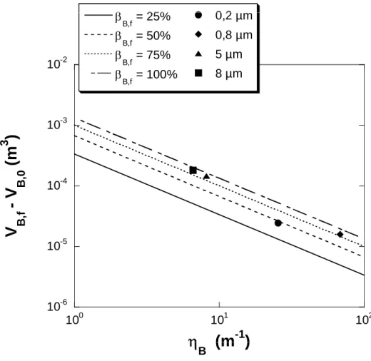
In Figure 7, we plotted

(

)

diameter effect has been studied (dpore = 0.2; 0.8; 5; 8 µm). Operating conditions were kept the

16

same for all these experiments: C = 10-2 _g.L-1_{, Δ}

P = 0.3 bar.

17

Only the 0.2 µm membrane displays a ‘high’ filtering surface open to the flow, close to 50%, 18

before the beginning of the regime dominated by the “cake formation”. The three other 19

membranes are very sensitive to fouling by surface blocking mechanism as their fraction of 20

surface open to flow is below 25% at the end of the blocking regime. The knowledge of the 21

ηB is therefore not sufficient to choose between different filter media as a low ηB parameter

22

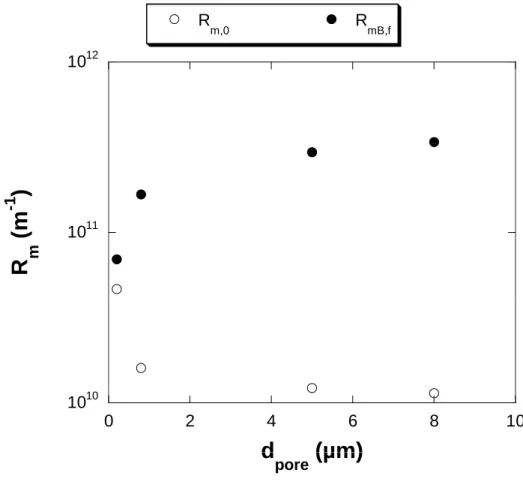
does not necessarily indicate a low fouling. Indeed, R_mB,f , the fouled filter media resistance at

the end of the blocking regime, is a key parameter in the filtration process. Figure 8 shows 1

two curves: 2

- the clean filter media resistance Rm_,0 versus dpore (○); 3

- the fouled filter media resistance R_mB,f versus dpore (●).

4

In Figure 8, the data which correspond to the 5 and 8 µm membranes are not considered in the 5

following discussion as we already know that a membrane whose mean pore diameter is way 6

greater than the particle size distribution should be avoided. 7

Usually, the choice of a filter media is usually made on the sole basis of the knowledge of the 8

clean filter media resistance, Rm_,0, value. In Figure 8, we can note that the 0.2 µm membrane 9

has a clean filter media resistance which is higher than the one of the 0.8 µm membrane 10

whereas, at the end of the blocking regime period, the former membrane displays a flux 11

resistance which is lower than the one of the latter. We can then deduce that the 0.2 µm 12

membrane is the best compromise and is able to maintain a good productivity during the cake 13

formation. 14

15

In short, the choice of a filter media, based on the methodology developed in this paper, 16

remains on the combination of three key parameters: 17

- the clean filter media resistance R_m,0;

18

- the ηB parameter;

19

- the filtrate volume during the blocking phase,

(

)

21

5.2. Blocking parameters variations when changing operating parameters

22 23

In this section, we focus on parameters variations for the system ‘bentonite suspension 1

– cellulose MF membrane’ with the two main mechanisms: complete blocking and cake 2

formation.

3 4

5.2.1 Effect of feed concentration 5

We conducted filtration experiments for a wide range of feed concentrations, from 10-3 to 10 6

g.L-1. The transmembrane pressure was set to 0.3 bar. 7

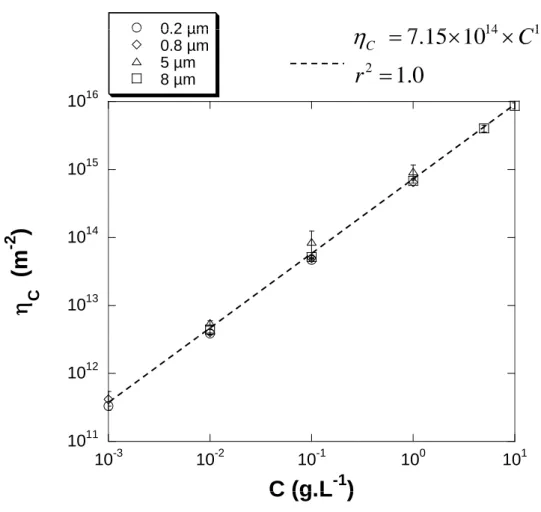
8

Figure 9 shows the increase in ηC the volumic specific resistance of the cake with bentonite

9

concentration for the four membrane pore diameters. A correlation can be determined: ηC =

10

7,2.1014×C1.1_{, whatever the studied membrane. which indicates that the value thus obtained}

11

characterizes the cake structure, and id independent on the filter characteristics. 12

As shown in Figure 10, ηBalso increases with the suspension concentration but in a nonlinear

13

way. This response could be explained by the presence of some interactions between the 14

particles and the filter media surface (when the concentration of particles is doubled, the ηB

15

value is not necessarily doubled) and particles steric hindrance at the pores entrance. Besides, 16

two zones can be distinguished according to the ratio of dpore (pore diameter) to dp (mean

17

particle diameter): the systems for which dpore ≤ dp and those for which dpore > dp.

18

We defined ψp/pore as the ratio of pore to particle projected surfaces (assuming spherical

19

particles). Physically; it represents the number of blocked pores quantity per blocking particle 20

when pore size is smaller than particle size.. 21 2 / p p pore pore d d ψ = ⎜⎛_⎜ ⎞⎟_⎟

⎝ ⎠ when dpore > dp, whereas

2 / pore p pore p d d ψ = ⎜⎛_⎜ ⎞⎟_⎟ ⎝ ⎠ when dpore ≤ dp. 22

When ηB is plotted versus C × ψp/pore (Figure11), data follow a same trend for concentrations

1

below 1 g.L-1. But for concentrations above 1 g.L-1, interactions between particles may play a 2

more significant role. 3

4

5.2.2 Effect of transmembrane pressure 5

6

The effect of transmembrane pressure on cake filtration parameter is investigated for the 7

range 0.03 - 1.2 bar. Two membranes are considered: 0.2 µm and C = 0.1 g/L; 8 µm and C = 8

1 g/L. Since (ηC) is proportional to C1.1, the sets of data for the two pore diameters (0.2 and 8

9

µm) can be normalised by dividing (ηC) by C1.1 (see § 6.2.1.). Data then fall on the same line

10

(Figure 12) which confirms that cake filtration is not influenced by the mean pore diameter of 11

the filter media. 12

As shown in Figure 13, (ηB) decreases when the transmembrane pressure increases for both

13

membranes (0.2 and 8 µm). In Figure 13, for the 8 µm membrane, the value of (ηB) is high

14

(1500 m-1) for very low transmembrane pressure, whereas it is much lower for the higher 15

pressures. This shows that bentonite particles have a strong tendency to stick to the membrane 16

pores at low filtration rate. The trend is different for the 0.2 µm membrane. As the mean 17

particle diameter is here four times greater than the mean pore diameter, the filtration rate has 18

a weak effect, compared to the 8 µm membrane. 19

From these data, we see that when increasing the transmembrane pressure, a decrease of the 20

ηB value has been observed .The shear stress, τw, at the pore entrance should be considered in

21

order to explain these observed variations. For a cylindrical pore, the shear stress, τw, at the

22

pore entrance is a function of the pore diameter, dpore, the fluid flow rate at the pore mouth, v,

23

and the fluid viscosity, µ . 24

pore w d v μ τ = 8 (14) 1 2

According to equation (14), we calculated the shear stresses (see Table 5) corresponding to 3 filtration experiments . 4 Table 5: 5 6 dpore (µm) ΔP (Pa) QB,0 (m 3_.s-1₎ v (m.s-1) Re τw (Pa) 0.2 120,000 5.45×10-7 5.08×10-4 1.02×10-4 20 30,000 3.67×10-7 _3.42×10-4 _6.84×10-5 ₁₄ 3,000 4.51×10-8 _4.20×10-5 _8.40×10-6 _1.7 8 120,000 3.01×10-6 2.81×10-3 2.25×10-2 2.8 60,000 2.48×10-6 _2.31×10-3 _1.85×10-2 _2.3 30,000 1.83×10-6 _1.70×10-3 _1.36×10-2 _1.7 9,000 8.02×10-7 _7.48×10-4 _5.98×10-3 _0.75 3,000 9.47×10-8 8.83×10-5 7.07×10-4 0.09 7

In Figure 14, we have plotted ηB versus the wall shear stress, τw. At low wall shear stress, ηB

8

has a high value, and conversely. This result is in good accordance with the fact that the effect 9

of a high wall shear stress at the pore entrance is to lift particles captured at the membrane 10

surface, in other words, to decrease the total amount of particles actually stick to in the filter 11

media. 12

Also, a threshold value for the wall shear stress (τw ≅ 2 Pa) appears in Figure 14, above which

13

ηB tends to stabilize when the transmembrane pressure increases. The data for the 0.2 µm are

all above the threshold value, which explains why the pore blocking mechanism is not as 1

much affected by an increase of transmembrane pressure as it is for the 8 µm membrane As 2

the average size of bentonite particle is around 0.5 μm; it can be expected that hydrodynamics 3

will only play a role when particle size are smaller than pores. Accounting for the shear stress 4

in the pore sheds some light, and some details on the physics of the particle capture efficiency 5

in this system. 6

7

5.2.3 Effect of pore diameter 8

9

Four microfiltration membranes have been tested (dpore = 0.2, 0.8, 5 and 8 µm).

10

Transmembrane pressure was set at 0.3 bar and the feed suspension concentration, C, at 10-2 11

g.L-1. 12

If we now consider the effect of the mean pore diameter on ηB, Figure 15 shows a maximum

13

for the 0.8 µm membrane for which dpore ≈ dp. This result confirms the fact that a maximum of

14

fouling by pore blocking can be reached when using a filter media with a mean pore diameter 15

close to the mean diameter of the particles of the suspension to be filtered. 16

We qualitatively compare Figure 15 to the particle size distribution of the bentonite 17

suspension presented in Figure 1. According to Figure 1, the quantity CB, the concentration of

18

all the particles which block pores of diameter dpore, is lower for dpore = 0.2 µm than for dpore =

19

0.8 µm. Figure 15 could be interpreted as the variation of CB with the mean pore diameter

20

dpore: the concentration of the potential particles which plug pores of diameter dpore varies

21

when using different membranes for a same given suspension. 22

23

6. Conclusions

24 25

A phenomenological approach, which includes a qualitative identification of the main 1

fouling mechanisms prior to a quantitative determination of parameters (blocking parameters) 2

characterising the “suspension-filter” system, allows a rather good description of the flux 3

decline and underlying fouling mechanisms during filtration of a particle suspension. We 4

have considered here the filtration of a bentonite suspension on several microfiltration 5

membranes over a wide range of feed concentrations and transmembrane pressures. 6

This work is based on splitting the fouling analysis into two steps: one is dedicated to 7

the identification of the prevailing fouling mechanisms, and the fraction of process they 8

control. This one much preferably will use equation (1), and the concept of capture efficiency. 9

The second step uses the integrated form of equation (1) and is aimed at finding the 10

values of the model parameters, for each fouling mechanism. 11

Even if several fouling phenomena may simultaneously occur, the assumption of 12

successive prevailing fouling mechanisms used here enables a good description of flux 13

decline during a filtration run. The good agreement between experimental and calculated data 14

over wide ranges of operating parameters is a favourable indication of the robustness to this 15

approach, even though the level of description of the filter-suspension system was kept as low 16

as possible all along which makes this approach quite a valuable one for complex systems 17

such as industrial suspension. As a matter of fact, time and volume filtered are the only basic 18

data used. Correlation to other information regarding the filter (pore size) or the suspension 19

(concentration, particles size distribution) is possible, but not necessary. 20

In the systems tested here, we identified two prevailing mechanisms namely surface blocking 21

and cake filtration. A valuable further step would be to extend this work to other systems 22

implying pore blocking as well as internal fouling by testing various “suspension-filter” pairs. 23

An original finding was that surface blocking may considerably reduce the filtering surface 24

open to flow, as up to 80% of the filter surface could get blinded at the end of the blocking 25

regime. Phenomenological correlations between blocking parameters for internal, surface or 1

cake blocking mechanisms and operating parameters such as feed concentration or pressure 2

give first insights into physical aspects which rule the particle trapping in different locations 3

of the filter. Such an approach should also be useful to develop more physical models for 4 blocking phenomena. 5 6 7 Acknowledgements 8 9

We would like to thank Rhodia Recherche for its financial support and its technical 10

expertise. 11

12 13

References

1 2

[1] Grace H.P., Structure and performance of filter media. I. The internal structure of filter 3

media, AIChE J., 2 (1956) 307-315. 4

[2] Hermia J, Etude analytique des lois de filtration à pression constante, Rev. Univ. 5

Mines., 2 (1966) 45. 6

[3] Hermans P.H. and Bredée H.L., Principles of the mathematical treatment of constant 7

pressure filtration, J. Soc. Chem. Ind. (1936) 1–4. 8

[4] Hermia J., Constant pressure blocking filtration laws. Application to power-law non-9

newtonian fluids, Trans. I. Chem. E., 60 (1982) 183.-187 10

[5] Hlavacek M. Bouchet F. , Constant flowrate blocking laws and an example of their 11

application to dead end microfiltration of protein solutions, J. Memb. Sci.., 82 (1993) 285.-12

297. 13

[6] Tracey E.M. and Davis R.H., Protein fouling of track-etched polycarbonate 14

microfiltration membranes, J. Colloid Interface Sci., 167 (1994) 104-116. 15

[7] Bowen W.R., Calvo J.I., Hernandez A, Steps of membrane blocking in flux decline 16

during protein microfiltration, J. Membr. Sci., 101 (1995) 153-165. 17

[8] Ho C.-C. and Zydney A.L., A combined pore blockage and cake filtration model for 18

protein fouling during microfiltration, J. Colloid Interface Sci., 232 (2000) 389-399. 19

[9] Combined models of membrane fouling: development and application to microfiltration 20

and ultrafiltration of biological fluids, J. Memb. Sci., 277 (2006) 75-84. 21

[10] Darcy H., Les fontaines publiques de la ville de Dijon; Victor Dalmont, Paris, 1856. 22

[11] Constantinides A., Finite difference methods, in Applied Numerical Methods with 23

Personal Computers, McGraw-Hill Book Company, New York, NY, 1987, pp. 275-319. 24

1

List of Symbols

2 3

A0 total membrane surface area (m2)

4

AB/mB blocked surface area of the membrane per unit of blocking particle mass (m2.kg-1)

5

C feed suspension concentration (kg.m-3)

6

Cv volume of the particles which uniformly deposit along the pore wall per unit of

7

permeate volume (dimensionless) 8

dp mean particle diameter (m)

9

dpore pore diameter (m)

10

k multiplicative constant in Eq. (1) (s1-n.m3n-6)

11

J permeate flux (m.s-1)

12

mC deposit mass per unit of membrane surface (kg.m-2)

13

n exponent in Eq. (1) (dimensionless)

14

ΔP transmembrane pressure (Pa)

15

Q permeate flow rate (m3.s-1)

16

QB,0 permeate flow rate at the start point of pore blocking (m3.s-1)

17

QI,0 permeate flow rate at the start point of internal fouling (m3.s-1)

18

Q0 initial permeate flow rate (m3.s-1)

19

Re Reynolds number (dimensionless)

20

R hydraulic resistance in Darcy’s law (m-1)

21

RC cake hydraulic resistance (m-1)

22

Rm membrane hydraulic resistance (m-1)

23

RmB fouled membrane hydraulic resistance by pore blocking (m-1)

24

RmB,f final fouled membrane hydraulic resistance by pore blocking (m-1)

1

Rm,0 clean membrane hydraulic resistance (m-1)

2

RmI fouled membrane hydraulic resistance by internal fouling (m-1)

3 4

V total volume permeated through the membrane at time t (m3)

5

VB,0 permeate volume value at the start point of pore blocking (m3)

6

VB,f permeate volume value at the end of pore blocking (m3)

7

VC,0 permeate volume value at the start point of cake filtration (m3)

8

v fluid velocity at the pore entrance (m.s-1)

9 t time (s) 10 11 Greek letters 12

α specific resistance of the cake (m.kg-1) 13

βB surface coverage ratio for pore blocking (dimensionless)

14

βB,f final surface coverage ratio at the end of the pore blocking regime (dimensionless)

15

εm membrane porosity (dimensionless)

16

εC cake porosity (dimensionless)

17

ηB blocked surface area by unit of time and surface (m-1)

18

ηC cake volumic specific resistance (m-2)

19

ηI vol. of particle accumulated per unit of permeate and unit of void volume (m-3)

20

μ permeate dynamic viscosity (Pa.s)

21

ρ permeate density (kg.m-3)

22

ρp particle density (kg.m-3)

23

τw shear stress ate the pore entrance (Pa)

ψp/pore blocked pores quantity by one blocking particle (dimensionless)

1 2 3

12 14

bentonite suspension after four settlings

(%

)

b

er o

f p

a

rt

ic

les

Num

b

Particle size (µm)

Particle size (µm)

1011

d

t/dV

(s

.m

)

d

dt/dV (s m

)

dt/dV (s.m )

Figure 2. Influence of the time step Δt on the k-value

determination by using the representation for the experiment using a 0.2 µm membrane (C = 10-2_{g/L and} Δ_{P = 0.3 bar)}

1011 1012

Step III

d

t/dV

(s

.m

)

Step I

Step II

d

dt/dV (s m

)

n = 2

_{n = 0}

n > 2

Figure 3. Example of the determination of the slope n in the representation for the fouling mechanisms identification ( experimental data for 5 µm membrane; C = 10-2_{g/L and}Δ_{P = 0.3 bar)}

dt/dV (s.m )

3 10-6 4 10-6 s -1 )

Q

(A)

(B) n =2

(B) n =2

V

(C) n = 0

V

Figure 4. Split of the curves into successive mechanisms: (A) very low fouling mechanism , ( B) blocking , (C) cake filtration.

2.5 10-4 3 10-4 3.5 10-4 0.2 µm (exp.) 0.2 µm (calc.) 2 10-4 2.5 10-4 3 10-4 0.8 µm (exp.) 0.8 µm (calc.) 0 100 5 10-5 1 10-4 1.5 10-4 2 10-4 0 500 1000 1500 2000 2500 3000 3500 4000 V (m 3 ) 0 100 5 10-5 1 10-4 1.5 10-4 0 500 1000 1500 2000 2500 3000 3500 V (m 3 ) t (s) t (s) 1.2 10-3 1.4 10-3 5 µm (exp.) 5µm (calc.) 2 10-3 8 µm (exp.) 8 µm (calc.) 4 4 10-4 6 10-4 8 10-4 1 10-3 V ( m 3 ) 5 10-4 1 10-3 1.5 10-3 V ( m 3 )

Figure 5. Plot of cumulative permeate volume V versus time t - comparison between

2 0 100 2 10-4 0 500 1000 1500 2000 2500 3000 3500 4000 t (s) 0 100 0 1000 2000 3000 4000 5000 t (s)

experimental and calculated curves for four experiments (C = 10-2_{g/L and} Δ_{P = 0.3}

0 2 µm (exp ) 1 1.2 0.2 µm (exp.) 0.2 µm (calc.) 8 µm (exp.) 8 µm (calc.) 0.4 0.6 0.8

β

ΔP (bar)

Figure 6. Effect of the transmembrane pressure ΔP on the final surface

coverage ratio, β_B,ffor two different membranes (0.2 µm and 8 µm)

β 25% 0 2 10-3 10-2 β B,f = 25% β B,f = 50% β B,f = 75% β B,f = 100% 0,2 µm 0,8 µm 5 µm 8 µm 10-4 103

V

- V

(m

)

V

η

(m

)

Figure 7. Symbols are the values of V_B,f– V_B,0versus η_B, for a series of data (d_pore= 0.2; 0.8; 5; 8 µm). Operating conditions were kept the same for all these experiments: C = 10-2

g.L-1_, Δ_{P = 0.3 bar. Lines are the calculated data of V}

B,f– VB,0versus ηB, for different

values of β_B,f

η

1012 R m,0 RmB,f 1011

R

(m

)

d

(µm)

Figure 8. Evolution of a clean and fouled filter media resistance (respectively, R_m,0 and R_mB,f) with its initial mean pore diameter, d_pore

d

0 2 µm * 14 1 1

7 15 10

C

7.15 10

1.0

C

r

η

=

×

×

=

η

(m

)

C (g L

)

Figure 9. Effect of feed suspension concentration C on the specific parameter, η_C, for cake formation at constant pressure 0.3 bar

0.2 µm 103 104 0.2 µm 0.8 µm 5 µm 8µm 101 102

η

(m

)

C (g L

)

C (g.L )

Figure 10. Effect of feed suspension concentration C on the specific parameter, η_B, for pore blocking at constant pressure 0.3 bar

103 104 0.2 µm 0.8 µm 5 µm 8 µm 102 103

η

(m

)

C x

ψ

(g L

)

C x

ψ

(g.L )

Figure 11. Plot of η_Bversus the product of feed concentration, C times the number of blocked pores per unit of blocking particle ψ (C×ψ ) at constant pressure blocked pores per unit of blocking particle, ψ_p/pore(C×ψ_p/pore) at constant pressure 0.3 bar

1 1 5 1015 2 1015 0.2 µm; C = 0.1 g.L-1 8 µm; C = 1 g.L-1 1

)

/ C

(m

kg

η

/

ΔP (bar)

Figure 12. Effect of transmembrane pressure on cake formation: comparison between two membranes (0.2 µm and 8 µm) by considering the plot of η_C/C1.1_versus Δ_P

ΔP (bar)

8 µm; C = 1 g.L-1 1500 2000 8 µm; C 1 g.L 500 1000 η B * (m -1 ) 0 10-2 10-1 100 101 ΔP (bar) 0.2 µm; C = 0.1 g.L-1 100 150 m -1 ) 0 50 10-2 10-1 100 101 η B * ( 102 101 100 101 ΔP (bar)

Figure 13. Effect of transmembrane pressure on pore blocking for two different membranes (0.2 µm and 8 µm) by considering the plot of η_B versus ΔP

1200 1400 1600 0.2 µm; C = 0.1 g.L-1 8 µm; C = 1 g.L-1 600 800 1000 1200

η

(m

)

τ (Pa)

Figure 14. Effect of the wall shear stress, τ_won pore blocking mechanism for two different membranes (0.2 µm and 8 µm)

τ

60 70 80 30 40 50 60

η

(m

)

d

(µm)

Figure 15. Effect of the mean pore diameter of the filter media on the specific parameter, η_B, for pore blocking (C = 10-2_{g/L and} Δ_{P = 0.3 bar)}

d