Capacity value of variable renewable energy and energy storage

Capacity Value of Variable Renewable Energy and Energy Storage

by

Conleigh Byers

B.S.E., Princeton University

Submitted to the Institute for Data, Systems, and Society and Department of

Electrical Engineering & Computer Science

in partial fulfillment of the requirements for the degrees of

Master of Science in Technology & Policy

and

Master of Science in Electrical Engineering & Computer Science

at the

MASSACHUSETTS INSTITUTE OF TECHNOLOGY

C Massachusetts Institute of Technology 2018. All rights reserved.

Author

Signature redacted

Technology 8(Policy Program, Electrical Engineering & Computer Science

August

Signature redacted

Certified by

Audun Botterud

Principal Research Scientist, Laboratory for Information and Decision Systems

Thesis Supervisor

Certifiedb

Signature redacted

Munther Dahleh

W. Coolidge Professor, Electric Engineering and Computer Science

Director, Institute for Data, Systems, and Society

Thesis Reader

Accepted by

Signature redacted

Munther Dahleh

W. Coolidge Professor, Electric Engineering and Computer Science

A bi eqor Institute for Data, Systems, and Society

Accepted by

Signature redacted_

_____

SECH

M'Leslie

A. Kolodziejski

Professor of Electrical Engineering and Computer Science

1

Chair, Department Committee on Graduate Students

MAL

U 1U 1i

LIBRARIES

ARCHIVES

Capacity Value of Variable Renewable Energy and Energy Storage

Conleigh Byers

Submitted to the Institute for Data, Systems, and Society and Department of Electrical Engineering & Computer Science

on August 10, 2018, in partial fulfillment of the

requirements for the degrees of Master of Science in Technology & Policy

and

Master of Science in Electrical Engineering & Computer Science

Abstract

Variable renewable energy (VRE) resources account for approximately half of new capacity additions in independent system operator (ISO) markets in the United States in the last five years. When designing and implementing capacity markets, system operators need to estimate future system capacity needs and often set maximum limits on the capacity different technologies can trade in the capacity market based on the expected contribution of each technology, including generation and demand, to system adequacy. Current capacity market designs often consider each resource independently, irrespective of the system's portfolio of resources, potentially overvaluing or undervaluing the capacity contribution of VRE and energy storage in the grid. We explore a method for calculating the standalone and integrated capacity value of an added VRE resource with existing energy storage resources. The difference between the integrated and standalone value is the portfolio effect, the additional capacity value gained by the synergy of VRE and the existing fleet. We also demonstrate a new method for translating a normalized expected unserved energy (EUE) target into required additional firm capacity and then into the standalone and integrated capacity values of an added VRE resource.

Thesis Supervisor: Audun Botterud

Title: Principal Research Scientist, Laboratory for Information and Decision Systems

Thesis Reader: Munther Dahleh

Title: W. Coolidge Professor, Electric Engineering and Computer Science Director, Institute for Data, Systems, and Society

Acknowledgments

The author acknowledges General Electric and the U.S. Department of Energy, Office of Energy Efficiency and Renewable Energy through its Wind Power Program for funding the research presented in this paper.

Contents

List of Figures List of Tables 1 Introduction

1.1 Problem description . . . .

1.2 Review of capacity market fundamentals . . . .

1.2.1 State of U.S. markets . . . .

1.2.2 Purpose of capacity markets . . . .

1.3 Future of capacity markets . . . . 2 Literature Review

2.1 Capacity value methodologies . . . .

2.1.1 Conventional capacity valuation . . . .

2.1.2 Capacity value of variable renewable energy resources . . . . . 2.1.3 Capacity value of energy storage resources . . . . 2.1.4 Integrated capacity value of VRE and energy storage resources 2.2 Review of current practice . . . .

2.2.1 Overview of U.S. markets . . . . 2.2.2 D iscussion . . . .

3 Methodology

3.1 Capacity adequacy standards . . . .

3.2 Standalone capacity value . . . .

7 9 11 13 . . . . 13 . . . . 14 . . . . 14 . . . . 17 . . . . 21 23 23 23 24 25 26 26 27 31 33 34 35

3.3 Integrated capacity value . . . 40

3.4 Portfolio effect . . . . 42

4 Dispatch model 43 4.1 Model description . . . 43

4.2 Model formulation . . . 44

4.2.1 Description of variables and parameters . . . 44

4.2.2 Problem formulation . . . 47

5 Case Study ₅₃ 5.1 Data sources ... ... ... .. 53

5.2 _{Results . . . 54}

5.2.1 Scenario descriptions . . . 54

5.2.2 Capacity values by reliability metric . . . . 55

5.2.3 Contributions to the portfolio effect . . . 64

5.3 D iscussion . . . . 65

6 Conclusion 69

List of Figures

1-1 Cost recovery via scarcity rents in energy markets . . . . 19

1-2 Missing money problem . . . . 20

1-3 Blackouts and inelastic demand in a competitive market . . . . 21

2-1 Effective load carrying capability . . . . 25

3-1 Capacity addition required to achieve LOLH target . . . . 36

3-2 Capacity addition required to achieve normalized EUE target . . . .. 36

3-3 Capacity addition required to achieve LOLH target and co-incident VRE gener-ation with NSE time periods . . . .. 37

3-4 VRE generation co-incident with NSE time periods reduces NSE . . . . 38

3-5 VRE generation netted off of NSE time periods . . . 38

3-6 NSE time periods reordered by magnitude . . . . 39

3-7 New capacity addition required to meet LOLP target . . . 39

3-8 Standalone capacity value of added VRE generation . . . 40

3-9 Capacity addition required to achieve LOLP target with new VRE generation included in dispatch simulations . . . . 41

3-10 Portfolio effect as difference between standalone and integrated capacity values using the LOLH criterion . . . 41

3-11 Portfolio effect as difference between standalone and integrated capacity values using the normalized EUE criterion . . . . 42

5-1 _{Base case dispatch results for two-day sample . . . 55}

5-2 Base case storage results for two-day sample . . . . 56

5-3 Integrated case dispatch results for two-day sample . . . .. 56

5-4 Integrated case storage results for two-day sample . . . . 57 5-5 Required additional capacity to meet adequacy standard of 2.4 LOLH per year

(Scenario 1) . . . . ....58

5-6 Required additional capacity to meet adequacy standard of 0.6 LOLH per year (Scenario 1) . . . . .58

5-7 Required additional capacity to meet adequacy standard of 0.4 LOLH per year (Scenario 1) . . . . 59 5-8 Required additional capacity to meet adequacy standard of 2.4 LOLH per year

(Scenario 2) . . . 59

5-9 Required additional capacity to meet adequacy standard of 0.6 LOLH per year (Scenario 2) ... ...

60

(Scenario 2) . . . . 61

5-11 ... ... .... 62

5-12 . . . . 6 2

5-13 Required additional capacity to meet adequacy standard of 0.0002% normalized EUE per year (Scenario 1) . . . 63 5-14 Required additional capacity to meet adequacy standard of o.oooi% normalized

EUE per year (Scenario 1) . . . 64

5-15 . . . . 65

5-16 Required additional capacity to meet adequacy standard of 0.0002% normalized EUE per year (Scenario 2) . . . 66 5-17 Required additional capacity to meet adequacy standard of o.oooi% normalized

EUE per year (Scenario 2) . . . 67 5-18 Required additional capacity required to meet LOLH targets with fixed energy

List of Tables

1.1 Comparison of general capacity market characteristics . . . . 16

2.1 Comparison of qualifying capacity valuation . . . . 29

2.2 Recent qualifying capacity values assigned to new resources . . . . 32

4.1 List of dispatch model variables and parameters . . . . 44

5.1 Capacity values by LOLH (Scenario i) . . . . 57 5.2 Capacity values by LOLH (Scenario 2) . . . . 6o

5.3 Capacity values by LOLH (Difference between Scenarios 2 and 1) . . . 6o

Chapter

1

Introduction

1.1

Problem description

Variable renewable energy (VRE) resources account for approximately half of new capacity additions in independent system operator (ISO) markets in the United States in the last five years. When designing and implementing capacity markets, system operators need to estimate future system capacity needs and set maximum limits on the capacity different technologies can trade in the capacity market based on the expected contribution of each technology, including generation and demand, to system adequacy. Current capacity market designs often consider each resource independently (irrespective of the system's portfolio of resources) and statically (without considering how the contribution may change as the system portfolio changes), potentially overvaluing or undervaluing the capacity contribution of VRE and storage in the grid.

Capacity market rules that assign the allowed capacity credit to individual units often follow heuristics that do not reflect true system value at scale for the different system resources, par-ticularly VRE and energy storage resources. Methods currently employed by nearly all ISOs in the U.S. assign qualifying capacity value of VRE resources based on historical assessments of output during administratively determined performance hours. These methods yield signifi-cantly different results for identical resources and fail to capture the correlation between VRE output and scarcity events (Byers, Levin, & Botterud, 2018). The measure is not predictive of

future capacity value when based on only one prior year of operating data, given the stochas-ticity of most VRE resources. Additionally year-on-year changes to the calculated value do not provide a consistent investment signal. If VRE capacity is over-credited, the ISO might buy less capacity than needed, leading to under-building other capacity resources and lower system reliability. However, under-crediting capacity is also inefficient, as it could lead to over-build of total generation capacity, under-utilization of some power plants, and possibly higher system cost than what is optimal. Inaccurate crediting can subsidize or penalize different resources,

distorting optimal investment decisions (Bothwell & Hobbs, 2017).

The complexity of assigning capacity values to VRE resources is exacerbated in systems with energy storage, including, e.g., pumped hydro storage and electrochemical batteries. There is an obvious complementarity between VRE and energy storage technologies, since in the presence of the latter, the variability and uncertainty of VRE resources become less of an issue.

A recent study demonstrated the potential of the existing hydropower system with reservoir

storage to increase the capacity value of additional wind and solar in the Pacific Northwest (Karier & Fazio, 2017).

We adapt a similar methodology to that used in Karier and Fazio (2017) to calculate an inte-grated capacity value of VRE generation and energy storage. We explore how the inteinte-grated capacity value with energy storage above and beyond the standalone capacity value of addi-tional VRE generation varies across reliability metrics and across differing reliability standards within a given reliability metric. We propose a new approach to translating a resource ade-quacy metric requiring a target total nonserved energy into a required additional firm capacity value. We then use this metric to calculate the integrated capacity value and portfolio effect of an added VRE resource to a system with existing energy storage.

1.2

Review of capacity market fundamentals

1.2.1

State of U.S. markets

A longstanding challenge in electric power systems has been the question of how to ensure

long-run resource adequacy and system reliability. In general, resource adequacy paradigms

1.2. REVIEW OF CAPACITY MARKET FUNDAMENTALS

can be categorized as traditional rate-of-return regulation and centralized planning, energy-only markets, and different forms of capacity markets and payments (Bushnell, Flagg, & Mansur, 2017; Hogan, 2005; Cramton & Stoft, 2006). In an ongoing debate over the necessity of specific capacity mechanisms covered extensively in the literature, proponents argue that imperfections in wholesale energy markets fail to achieve a least-cost portfolio of resources that satisfy consumer reliability preferences (Joskow, 2008; Cramton & Stoft, 2006).

A number of reviews of capacity markets in the United States exist (e.g., Bushnell et al. (2017),

Bhagwat, de Vries, and Hobbs (2016), Porter, Starr, and Mills (2015), and FERC (2013)). PJM,

ISO-NE, MISO, and NYISO are independent system operators/regional transmission

organiza-tions (ISOs/RTOs) that all operate centralized capacity markets. Table 1.1 summarizes general characteristics of these markets, illustrating differences in capacity procurement methods, auction procedures, and products. Note that ISO-NE bundles capacity obligations with finan-cial call options to supply energy when the energy price rises above a specified strike price (ISO-NE, 2016c). In this sense, the ISO-NE capacity market is similar to a so-called reliability options model, as proposed by Vazquez, Rivier, and Perez-Arriaga (2002) and Oren (2005), while PJM, NYISO, and MISO all conduct forward capacity markets. Among the other regional electricity markets in the United States, CAISO and SPP also impose resource adequacy re-quirements on load-serving utilities but without a centralized capacity market. In contrast, ERCOT relies on an energy-only market with high price caps and a real-time price adder that reflects the marginal value of available operating reserves to provide incentives for investments and resource adequacy.

Table 1.1: Comparison of general capacity market characteristics*

* _{Table adapted from Byers et al. (2018)}

ISO Capacity Pro- Auctions Planning Zonal Re- Must Offer

curement Horizon quirements and Bidding

Provisions PJM Centralized 1. Base Resid- 1. 3 years System-wide Must offer

market ual Auction prior to an- price zone into day-Forward Con- 2. Incremental nual delivery plus 12 Loca- ahead market tract Auction 2. 20,10, and 3 tional Delivery (DAM)

months prior Areas (sub-to annual de- zones). No di-livery rect mapping

to PJM load zones

ISO-NE Centralized 1. Forward Ca- . 3 years System-wide Must offer market pacity Auction prior to an- price zone and into DAM and Capacity con- 2. Annual Re- nual delivery 2 subzones 1. real-time mar-tract with fi- configura- 2. 24, 8, and 3 South East ket (RTM), nancial call tion Auctions months prior New England must schedule option for en- (ARA1, ARA2, to annual de- 2. Northern maintenance ergy ARA3) livery New England with ISO

3. Monthly 3. 2 months

Reconfigura- prior to tion Auction monthly

1.2. REVIEW OF CAPACITY MARKET FUNDAMENTALS RA Require-ment: Bilat-eral contracts or voluntary centralized market Forward Con-tract Centralized market Forward Con-tract Planning Re-source Auction 1. Capability Period Auc-tion/Strip Auction (6 months) 2. Monthly Auction 3. Spot Mar-ket Auction 1 year prior to annual deliv-ery 1. At least 30 days prior to each 6 month delivery pe-riod 2. For any remaining month in 6 month capa-bility period 3. For upcom-ing month only io Local Re-source Zones,, each with sep-arate require-ment System-wide New York Control Area zone and three sub-zones

Must offer full

cleared un-forced capac-ity into DAM, with exception for scheduled maintenance. Also applies to VREs and participating external re-sources Resources must offer their unforced capacity into the DAM

1.2.2

Purpose of capacity markets

Different forms of capacity remuneration mechanisms (see (Bushnell et al., 2017; Hogan, 2005; Cramton & Stoft, 2006)) that are coupled with energy markets may include bilateral contracts, capacity payments, strategic reserves, and long-term energy auctions, among others, in addition to centralized capacity markets. Proponents of capacity markets in particular

MISO

NYISO

i i i i i

argue that market imperfections cause energy-only markets to fail. While in the long-run without intervention, this contention may predict more dire consequences for energy-only markets, the concern fundamentally is one of efficiency. This line of argument says that market imperfections cause energy-only markets to fail to achieve a least-cost portfolio of resources that satisfies consumer reliability preferences. Empirically, we see both energy-only and capacity market approaches can suffice. Another framing tool by which to look at this debate is through the lens of a risk-cost trade-off. For example, an energy-only approach may require more operator intervention in the form of increased operating reserves or some other means that meets consumer reliability standards with a higher risk of failure than an idealized system with a fully-functioning capacity market. Ultimately, if system operators are rather risk-averse and willing to intervene, reliability outcomes in systems with and without capacity markets may be similar, with simply a difference in the economic efficiency of achieving the given standard.

Ideally, short-term marginal prices in an energy market provide optimum investment signals (Schweppe, Caramanis, Tabors, & Bohn, 1988). The optimality conditions of an ideal central-ized market maximizing social welfare are the same as the optimality conditions of a perfectly competitive market. Figure 1-1 illustrates the importance of scarcity rents in achieving cost recovery. In a market where each firm bids its marginal cost, the market will be in equilibrium when the net present value of the sum of the scarcity rents, the difference between the market clearning price and the marginal cost of each type of generation, across the lifetime of the asset equals its cost of capital. In Figure 1-1, the scarcity rent A for the highest marginal-cost asset is shown. From this example, it is clear that prices must be allowed to rise higher than the highest marginal cost of generation, as otherwise this asset would not be able to recover its fixed costs.

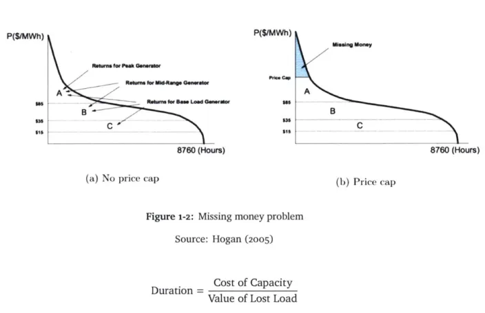
Perhaps the most-cited imperfection in energy markets leads to the 'missing money' problem due to price caps, in which cost recovery is not possible through marginal cost pricing alone. Figure 1-1 illustrates the existence of a price cap, one form of regulatory price suppression, that would provide insufficient scarcity rents to achieve cost recovery. Figure 1-2 demonstrates a similar price cap leading to missing revenues needed to achieve cost recovery via a load duration curve over the course of a year. In the short-term, demand does not set the scarcity price because of limited demand-response: there may exist price caps or offer caps, and the system operator may intervene to prevent emergency conditions from occurring that would

1.2. REVIEW OF CAPACITY MARKET FUNDAMENTALS

Demand

Price Cap _X

Supply

MW

Figure i-i: Cost recovery via scarcity rents in energy markets

drive the price adequately high for cost recovery. Inefficient pricing may also be present because of price caps and non-convex costs. In the long-term, other factors may contribute to insufficient investment: generators are risk-averse and may not build if they do not think scarcity rents will be allowed to rise high enough. Other factors that inhibit a perfectly competitive energy market include investments that are not continuous ("lumpy" investments) and the existence of economies of scale.

However, the argument for the existence of capacity markets does not only depend on the factors examined above that may lead to insufficient cost recovery and thus inadequate capacity in the long-run, barring additional regulatory intervention. Capacity markets are also proposed as a means to overcome the problem of inelastic demand. Beyond regulatory price interference, there are demand-side market failures. Cramton, Ockenfels, and Stoft (2013) conceptualize the adequacy problem as providing the amount of capacity that optimizes the duration of blackouts.2 Capacity should be built until the marginal cost of capacity equals the marginal reduction in the cost of lost load, which we may write as

2_{Note that common engineering reliability standards, e.g., i day in lo years) do not necessarily reflect the}

underlying economic trade-off between cost and reliability consistent with consumer preferences.

P(S/MWh) sm $sI P($/MWh) P.c CEP W. us5 $sI

tRourm for PeakGnrar_{Reowrne for MWd~Ang Genelor}

A Un e GnML

B

8760 (Hours)

(a) No price cap _{(b) Price cap}

Figure 1-2: Missing money problem Source: Hogan (2005)

. Cost of Capacity Value of Lost Load

Since the cost of capacity is positive and the value of lost load is positive, the optimal duration of blackouts must also be a positive number greater than zero. However, while we are able to calculate the optimal duration of blackouts, there is no competitive market price during blackouts due to inelastic demand. Figure 1-3 demonstrates that during a blackout, a portion of demand is perfectly inelastic and thus does not intersect the supply curve. With increasing technological innovation, this demand-side flaw may be mitigated. Cramton et al. (2013) and other proponents of capacity markets would argue that while economics can tell us the optimal duration of blackouts, it does not tell us the optimum level of capacity that results in the specified duration of blackouts. This problem is principally the purview of engineers and the reason behind the necessity of calculating capacity value, explored further in Chapter 2.

W@ns Mooney A B C 8760 (Hours) in [

1.3. FUTURE OF CAPACITY MARKETS

Blackout

Price

A

Peaker

Supply

Demand

Marginal Cost

Baseload

Marginal Cost

Power

1-3:

Source: Cramton, Ockenfels, and Stoft (2013)

1-3

Future of capacity markets

Capacity mechanisms continue to evolve both in the U.S. and elsewhere. The U.S. has four centralized capacity markets in addition to various other capacity requirements in, e.g., CAISO and SPP. A number of nations in Europe have recently moved away from energy-only market approaches (Feuk, 2015). Additionally, even a nominally energy-only market like ERCOT has designs that diverge from the pure energy-only approach discussed above. For instance, ERCOT's operating reserve demand curve, a real-time energy price adder, increases the times in which the scarcity price prevails (Value of real-time reserves = Value of avoiding load-shed) without the system actually going into emergency conditions (ERCOT, 2014). The ORDC is a probabalistic assessment that also increases prices during times without scarcity since there is still a probability that a scarcity event may occur.

Nevertheless, the future of capacity markets is uncertain. Concerns have been raised about the cost-effectiveness of capacity markets. The U.S. Government Accountability Office recently recommended FERC assess overall performance of capacity markets as a long-run resource adequacy approach, citing high costs of capacity markets and little by way of metrics to 21

evaluate their added value (GAO, 2017).

Additionally, there exist open questions regarding whether capacity markets should allow VRE and storage to participate and if so, how.3 Currently, concerns over low capacity market prices driven by renewable resources - and partly exacerbated by subsidies -have led

ISO-NE to introduce a proposal for a two-settlement capacity auction (ISO-ISO-NE, 2017). The first

round of the capacity market would include a minimum offer price rule that would limit the participation of most VRE resources, but retirement offers below the clearing price would receive a supply obligation. The second auction would take place without a minimum offer price or demand curves but a quantity fixed at the amount of capacity re- presented by the cleared retirement offers from the first auction. The clearing price of the second auction would be the transfer price between the two auctions. ISO-NE argues that its proposed two-settlement auction process will relieve the downward pressure that subsidized resources are putting on capacity prices. PJM is also exploring new capacity market constructs that take into account state subsidies, particularly for nuclear plants (PJM, 2017d). However, it is less clear what purpose maintaining higher capacity prices serves when additional capacity has been procured due to state subsidies, especially if this leads to over-supply of capacity. Care should be taken to ensure that capacity markets are allowed to provide signals for resources to also exit the market when this makes economic sense and does not reduce reliability below desired levels. If a system operator is concerned that insufficient capacity is being procured in the capacity market, the resource adequacy metric should be revisited. As VRE and energy storage capacities grow and capacity markets continue to evolve, more attention must be given to how to properly integrate these resources into capacity markets.

3

Chapter

2

Literature Review

There is a potential complementarity between VRE and energy storage resources. Variability and uncertainty of VRE resources may become less of an issue with storage, as storage can shift VRE generation to critical hours. However, capacity markets often consider each resource independently, irrespective of the system's portfolio of resources, and statically, without con-sidering how the contribution may change as the system portfolio changes. Current methods potentially over- or under-value the capacity contribution of VRE and storage resources. Ca-pacity value of VRE is almost exclusively calculated via average-output during performance hours, often for only the prior year. This is more of a historical assessment than one predictive of future firm capacity contribution, and does not provide a good investment signal, since the value is so uncertain. The capacity value of energy storage resources is mostly undefined in current markets.

2.1

Capacity value methodologies

2.1.1 Conventional capacity valuation

Calculating the capacity value of conventional thermal resources is fairly well-established. The 'unforced' (in contrast to nameplate) capacity may be calculated via some variation of a forced outage rate and convolution (Billinton & Allan, 1996). Correlation between units

is ignored in this analytical approach, while correlation between VRE resources via weather patterns is significant. This method also discards chronological information, which affects energy storage resources. Discarding chronological information is a valid simplification for a thermal-dominated system, in which capacity and failure rate are dominant characteristics that have small variance in time. However, it is not possible to scale up one time interval without violating the operating conditions of storage, since the energy constraint changes with time. Treating VRE as negative load could lead to an overbuild of other types of capacity, increasing total costs, as it may be more efficient to curtail some VRE. Optimized operation of energy storage resources depends on more than just its own parameters, including load, VRE, and thermal generator constraints. The capacity value of an energy storage resource CES(t) can be thought of as a function of deterministic parameters KES (e.g., installed capacity), stochastic inputs KES _{(e.g., water inflow for a hydro plant), as well as load L(t), VRE generation CVRE(t),}

and thermal generator parameters CT(t).

CES(t) =

f(KES,

The least-cost capacity expansion solution depends on the operation of the other units.

2.1.2 _{Capacity value of variable renewable energy resources}

The Effective Load Carrying Capability (ELCC) method can be used to determine the marginal qualifying capacity contribution of a resource in a static system. ELCC is the preferred calcu-lation methodology of an IEEE task force for wind capacity value (Keane et al., 2011). This approach is supported in a number of studies examining different reliability metrics, e.g., Ibanez and Milligan (2014), Milligan et al. (2016). The principles for calculating ELCC were developed as early as in Garver (1966). With the ELCC method, a Loss of Load Probability (LOLP) is summed up over a time period, typically one year, to yield the Loss of Load Ex-pectation (LOLE). A target LOLE value is chosen, and two cases are considered, one with the additional generation resource and one without the additional generation resource. The load is adjusted to preserve the same LOLE target in the two cases. The ELCC is calculated as this incremental load served by the additional resource. Figure 2-1 illustrates this method.

ELCC is a marginal accounting that relies on convolution of the existing fleet's forced outage

2.1. CAPACITY VALUE METHODOLOGIES

where chronological information becomes important. This method also does not take into account potential synergy between VRE and energy storage resources. Inaccurate crediting can subsidize or penalize different resources, distorting optimal investment decisions (see, e.g., Bothwell and Hobbs (2017)).

0.14 -(U _j 0 -j 0.12 0.1 0.08 0.06 0.04 0.02 0 8000

0----+-Original Reliability Curve

-4-After Adding New

Generation

-*-Target Reliability Level

SI I I

8500 9000 9500

Load (mW)

10000 10500 11000

Figure 2-1: Effective load carrying capability The effect of an additional generator on LOLE is shown. Source: Keane et al. (2011)

2.1.3

Capacity value of energy storage resources

Previously, analytical methods have been proposed to estimate the contribution of energy storage to system reliability, although these approaches necessarily require unrealistic operat-ing simplifications. For instance, Klockl and Papaefthymiou (2005) assume unlimited storage

capacity, and Edwards, Sheehy, Dent, and Troffaes (2017) ignore charging constraints. Hu,

Karki, and Billinton (2009) use sequential Monte-Carlo methods, which help to capture the

importance of chronological information, but the dispatch logic is simplified in a manner 25

that doesn't fully account for system cost considerations. Sioshansi, Madaeni, and Denholm

(2014) use a dyanmic programming approach to maximize arbitrage profit with perfect price

foresight.

2.1.4 Integrated capacity value of VRE and energy storage resources

A recent study demonstrated the potential of an existing hydropower system to increase the

capacity value of additional wind and solar in the Pacific Northwest, calculating an integrated capacity value for wind and solar due to the ability of storage to move generation to time periods in which it had more value (Karier & Fazio, 2017). The authors use the adequacy standard adopted for the Pacific Northwest by the Northwest Power and Conservation Council. Under this adeuqacy standard, any simulation in which there is nonserved energy (NSE) counts as an adequacy miss. Some number of simulations is run, each accounting for different stochastic inputs. The number of adequacy misses divided by the number of simulations is defined as the loss of load probability (LOLP) of the simulation horizon. For instance, if the standard is an annual LOLP of 5% and 100 simulations of one year of operation are run, then 5 misses are allowed (--L = .05). This contrasts to other LOLP approaches that count adequacy

misses daily or hourly. Under the approach of Karier and Fazio (2017), the capacity required to meet the adequacy standard can be calculated by selecting the highest curtailment hour from each annual simulation and ordering them from highest to lowest magnitude. Following

NERC conventions, we may translate this measure into expected loss of load events (LOLEV) of .05 per year (NERC, 2016). This approach is compared to the methodology used in this

work in Section 3.1 and Section 5.2.2.

2.2

Review of current practice

The variable and uncertain generation of wind and solar resources requires specific considera-tion in terms of estimating how these resources contribute to system adequacy and the amount of capacity they should be allowed to bid into capacity markets. The fraction of name-plate capacity that is considered to be qualifying capacity for VRE differs by market and resource

1

2.2. REVIEW OF CURRENT PRACTICE

type. While a number of methods have been proposed to calculate the capacity value of wind power (e.g., Ibanez and Milligan (2014), Keane et al. (2011), Milligan et al. (2016), most jurisdictions calculate the qualifying capacity value of VRE resources based on their historical output during performance hours, which may correspond to peak load or times of likely short-age conditions. Recent work indicates that inaccurate valuing of capacity of wind and solar may significantly influence market efficiency (Bothwell & Hobbs, 2017). The growth of VRE

could also motivate more investment in energy storage resources. Future market designs will therefore also need to take into consideration the interaction of VRE and storage, including hydro, when determining contributions to system reliability.

2.2.1 Overview of U.S. markets

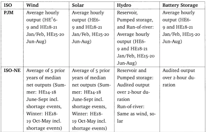
PJM calculates the qualifying capacity of VRE and energy storage resources from the average

hourly output during expected performance hours in winter and summer (PJM, 2017b). Wind and solar resources will be assigned a capacity value that is the average of three prior summer capacity values during performance hours (PJM, 2017c). For resources with less than three years of operating data, PJM uses a class average capacity factor determined by PJM for each summer of missing or incomplete data.

ISO-NE also calculates summer and winter qualifying capacity for existing wind and solar

resources based on the average of historical median output levels during performance and shortage hours over the previous five years (ISO-NE, 2016c). When determining the qualifying capacity of new wind or solar resources, ISO-NE uses an internal tool that considers project site conditions and data submitted by asset owners. ISO-NE had not qualified any battery resources by April 2017 but plans to qualify such resources as non-intermittent generators in similar fashion to conventional and pumped hydro (ISO-NE, 2016b).

MISO uses the ELCC approach to determine the qualifying capacity contribution of wind resources (MISO, 2016). MISO uses a LOLE target of i day in lo years, or o.1 days/year, in an annual calculation for each wind resource using the eight highest coincident-peak load hours of the year. A system-wide ELCC of wind resources is also calculated for new wind projects. The qualifying capacity of solar resources is based on the average output during summer performance hours for the prior three years. Units without a minimum of 30 consecutive days of operating data including these performance hours receive the system solar qualifying

capacity, calculated at 50 percent for 2016-2017. The qualifying capacity of reservoir and pumped storage hydro is determined by measuring the median head in summer performance hours over the past 5-15 years and converting to expected power output. A method for determining the qualifying capacity of batteries has not yet been specified.

NYISO calculates the qualifying capacity of wind and solar resources based on average output

during summer and winter performance hours in the previous six-month delivery period (NYISO, 2017). The qualifying capacity of reservoir and pumped storage hydro is the station-wide average output over a 4-h period with average stream flow and storage conditions. A methodology for determining qualifying capacity for batteries has not yet been specified.

CAISO does not have a centralized capacity market but does have regional resource adequacy

requirements. The ISO calculates the capacity value of wind and solar using an exceedance methodology to calculate 12 final monthly values, averaged over 3 years of production data

(CAISO, 2015). The value is based on the generation amount that a resource produces at

least 70 percent of the time during the performance hours, which vary seasonally. Added to this exceedance value is a share of the System Diversity Benefit. The monthly diversity benefit is the difference between the 70 percent exceedance of all wind (solar) resources as a group and the sum of the qualifying capacities of all individual resources. The share of the diversity benefit is the diversity benefit multiplied by the MWh produced during the included hours by that resource divided by the MWh produced by all wind and solar resources during the included hours. For new resources or resources with less than three years of operating data, missing monthly qualifying capacity values are calculated. The substituted value is the average calculated qualifying capacity of all existing wind (solar) resources in that month as a fraction of the available capacity of all existing wind (solar) resources in that month. CAISO calculates the available capacity of all same-technology resources as the 1 percent exceedance value of all hours in the month. Pumped hydro is treated as a dispatchable resource for qualifying capacity calculations, submitting a proposed value based on its tested maximum output and a deliverability assessment during a resource shortage condition performed by

CAISO. A methodology is not yet outlined for battery storage resources.

While ERCOT does not have a resource adequacy requirement, the ISO conducts analyses of the impacts of wind on reserve levels and reliability (ERCOT, 2015). To determine the system total capacity estimate in connection with the planning reserve margin, wind capacity during peak summer and winter loads is derated by the seasonal peak average available capacity

2.2. REVIEW OF CURRENT PRACTICE

during the 2o-highest system peak load hours for the season. The derated wind capacity is the average of up to io years of seasonal averages. For solar, 100 percent of the nameplate capacity of the first up to 200MW is used, and additional solar contributing capacity is calculated as the average capacity available during the highest 20 peak load hours for the prior three years. Hydro capacity contributions toward peak is the average capacity available during the 20

highest peak load hours for the prior three years. An ELCC methodology was used in 2013 to determine the capacity value of wind. Using fifteen years of hourly wind and load profiles, ERCOT assigned coastal wind a capacity value of 32.9 percent and western wind a value

of 14.2 percent (ECCO, 2013). No capacity value studies for battery storage resources were

found.

Table 2.1: Comparison of qualifying capacity valuation*

ISO Wind Solar Hydro Battery Storage

PJM Average hourly Average hourly Reservoir, Average hourly output (HEt6- output (HE6- Pumped storage, output

(HE6-9 and HE18-21 9 and HE18-21 and Run-of-river: 9 and HE18-21

Jan/Feb, HE15-20 Jan/Feb, HE15-20 Average hourly Jan/Feb, HE15-20 Jun-Aug) Jun-Aug) output (HE6- Jun-Aug)

9 and HE18-21

Jan/Feb, HE15-20 Jun-Aug)

ISO-NE Average of 5 prior Average of 5 prior Reservoir and Audited output years of median years of median Pumped storage: over 2-hour du-net outputs (Sum- net outputs (Sum- Audited output ration

mer: HE14-18 mer: HE14-18 over 2-hour du-June-Sept incl. June-Sept incl. ration

shortage events, shortage events, Run-of-river: Winter: HE18- Winter: HE18- Same as wind,

so-19 Oct-May incl. 19 Oct-May incl. lar shortage events) shortage events)

ELCC based

on 8 highest coincident-peak load hours of the preceding year

Average output (Summer:

HE14-18 Jun-Aug,

Win-ter: HE16-2o Dec-Feb) of preceding delivery period

Average hourly output (HE15-17 Jun-Aug) for prior

3 years

Average output (Summer:

HE14-18 Jun-Aug, Win-ter: HE16-2o Dec-Feb) of preceding delivery period

MISO Reservoir and Pumped Storage: Median head in prior 5-15 years (HE15-17 Jun-Aug) converted to expected output Run-of-river: me-dian output from prior 3-15 years (HE15-17 Jun-Aug) Reservoir and Pumped Storage: Average output over 4-hour pe-riod with average stream flow and storage conditions Run-of-river: av-erage output dur-ing 20 highest load hours in prior 5 capability periods (Winter: Nov-Apr, Sum-mer: May-Oct) NYISO Not defined Not defined

2.2. REVIEW OF CURRENT PRACTICE

CAISO Monthly 70% ex- Monthly 70% ex- Reservoir and Not defined ceedance value ceedance value Pumped Storage:

(averaged over (averaged prior Assessed max out-prior 3 years, last 3 years, HE17- put under

short-HE17-21 Nov-Mar, 21 Nov-Mar, HE14- age condition HE14-18 Apr-Oct) 18 Apr-Oct) + Run-of-river:

+ Share of system Share of system Same as wind, so-diversity benefit diversity benefit lar

of wind of solar

ERCOT ELCC with 15 All of first _{(Type unspeci- Not defined}

years of data; Av- 200MW; then, av- fied): Average erage of up to io erage available available capacity years of seasonal capacity during during 20

high-average capacity highest 20 peak est load hours for

during 20 high- load hours for _{prior 3 years}

est load hours for prior 3 years summer and

win-ter

* The PJM, ISO-NE, MISO, and NYISO portions of this table are drawn directly from Byers et al. (2018)

Hour Ending (HE) refers to the time at the end of each operating hour. For example, the operating period from 2:00pm to 3:OOpm is HE15.

2.2.2 Discussion

Table 2.1 summarizes the qualifying capacity evaluation procedures for VRE, hydropower, and batteries in the four different centralized capacity markets plus CAISO and ERCOT. Qualifying capacity calculations are primarily based on historical average output during a small number of peak system hours, often for the prior year only. This method could yield significantly different values year-to-year and between ISOs given the stochastic nature of wind and solar production. This method is unlikely to provide a good investment signal, since it is more of a historical assessment than predictive. The ELCC method employed by MISO and ERCOT for

wind better captures the correlation between load and wind output, but MISO and ERCOT both still rely on average hourly output for solar.

Table 2.2 compares the qualifying credits applied to new wind and solar resources in recent auctions. While we may expect to see a large spread of values varying by specific VRE resource and geographical location, it is unclear how reflective the wide range of values attained is of underlying value to the system. Notably, solar tends to be valued more highly than wind by these calculation methodologies.

Increased energy storage penetration will require careful consideration of how to properly credit a mix of VRE and storage, as storage technologies can be used to ensure delivery of energy from VREs during peak demand hours. Currently, most markets do not distinguish between reservoir and pumped storage hydro. CAISO's exceedance methodology and system diversity benefit share stand out, but it is unclear if this method of distributing a positive portfolio effect of capacity value is optimal. Only PJM and ISO-NE have explicitly defined methodologies for quantifying qualifying capacity from batteries. Future analysis may inves-tigate the possibility of allowing market participants to determine their own capacity offer commiserate with anticipated penalties.

Table 2.2: Recent qualifying capacity values assigned to new resources *

ISO Wind Solar

PJM 14.7-17.6% 38%-60%

ISO-NE 9-18% (summer) 27-33% (summer)

MISO 15.6% 50%

NYISO io% (summer) 26-46% (summer)

30% (winter) 0-2% (winter)

38% (offshore,

both seasons)

Ranges reflect different system configurations or geographic locations. References: PJM (2017a),

ISO-NE (2014), ISO-NE (2016a), MISO (2016), NYISO (2017)

Chapter 3

Methodology

This section describes a method for calculating the integrated capacity value of VRE resources in systems with energy storage and isolating the portfolio contribution to this value. Karier and Fazio (2017) propose a method of calculating the standalone and integrated capacity value of added VRE resources with a large existing hydropower fleet. We generalize this method to energy storage resources, adapt new reliability metrics, and explicitly explore the contribution of energy storage resources to the difference in value between the standalone and integrated capacity values, which we call the portfolio effect. We also propose a new method of converting the normalized expected unserved energy (EUE) metric for reliability to a capacity value. Chapter 5 explores numerical results in a simulated system using this method and the dispatch model described in Chapter 4.

In this method, both a standalone and an integrated capacity value is calculated for a marginal addition of VRE generation. A number of simulations must be run due to the stochastic but often-correlated nature of unit outages, load, and VRE generation, among other factors. The standalone value represents the capacity value of the resource, holding the operations of other units fixed. The integrated value represents the capacity value allowing for changes in the operation of existing resources. For instance, the energy storage resources may more optimally distribute the VRE over the time periods in the horizon under consideration. This would lead to a higher integrated value than standalone value. The difference between the integrated and standalone value is the portfolio effect, the additional capacity value gained by the synergy of

VRE and the existing fleet. The entire fleet should be considered in this portfolio effect if all units are allowed to change their operations in response to the new VRE generation. By fixing the output of energy storage resources to levels prior to the introduction of the additional VRE resource, we can isolate the contribution of energy storage resources to the portfolio

effect.

3.1

Capacity adequacy standards

We calculate an hourly loss of load expectation (LOLE), often referred to as loss of load hours (LOLH). The loss of load probability (LOLP) is conventionally calculated as using the peak load hour of each day (Billinton & Li, 1994; Ibanez & Milligan, 2014). LOLE typically refers to daily LOLE, the expected number of days per year in which available generation capacity is insufficient to meet the peak daily demand (NERC, 2016). Meeting peak demand does not imply meeting demand in other hours of the day with significant shares of VRE resources,

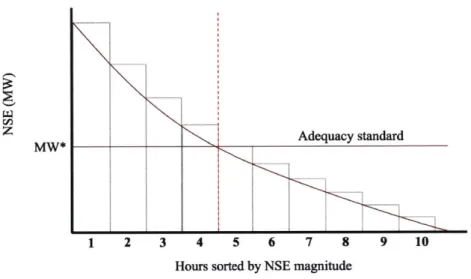
so an hourly LOLE (LOLH) may be a more suitable metric. A common industry standard for daily LOLE is 1 day in 10 years. Note that this daily LOLE standard of .1 events per year is not equivalent to 2.4 hours per year of unmet load (Keane et al., 2011; NERC, 2016). To translate daily LOLE to the expected number of hours in which available capacity is insufficient to meet load, we must assume an average duration of shortage events. The examples that follow assume a yearly LOLE of .1 and an average outage duration of 4 hours. If io yearly simulations at an hourly resolution are run, this translates to an hourly LOLE or LOLH of 4 hours. When calculating the additional capacity required to meet the LOLH target, all hours with nonserved energy (NSE) from all simulations are ranked by magnitude from highest to lowest, from left to right.1 The intersection of the target LOLH and the NSE curve is the capacity required. Figure 3-1 shows the corresponding required capacity MW* to meet an adequacy standard of

.4 LOLH per year with io yearly simulations (4 hours in io years).

While hourly LOLE accounts for the total duration of outages, neither of these metrics dis-tinguish between the magnitude of the nonserved energy in a shortage event. For instance,

LOLE would not distinguish between an hour with 20 MWh unserved energy and an hour with

'Note that Karier and Fazio (2017) use only the highest curtailment hour from each simulation instead of all nonserved energy hours due to the use of a different reliability metric. This metric is similar to a yearly loss of load events (LOLEV) metric.

3.2. STANDALONE CAPACITY VALUE

2000 MWh nonserved energy. Similarly, LOLE does not distinguish between system size; more

consumers are likely to experience a 2000 MWh outage in a given hour in a smaller system

than in a larger one. An alternative reliability metric is the normalized expected unserved energy (EUE), the expected number of megawatt hours of load not met by existing capacity normalized by the total megawatt hours of load (Pfeifenberger, Spees, Carden, & Winterman-tel, 2013; NERC, 2016). Normalized EUE may be expressed as an overall percentage of system load that cannot be served by existing capacity, e.g., 0.002% per year. By multiplying by the total megawatt hours of load and the number of yearly simulations, the allowable EUE target can be found. At the capacity level required to meet the target, the area under the NSE curve and above this capacity level will be equal to the EUE target, as shown in Figure 3-2. This level is found by searching through capacity levels C from the highest NSE value of each NSE curve and incrementally decreasing C in each iteration. The desired level MW* is found by taking the integral from hour 1 to the hour of intersection between the current capacity level C with the NSE curve, hour H. The difference between this value and the product of C * (H - 1) (note

that f(NSE) is a step function) yields the shaded area. When the shaded area is equal to the

EUE target EUE*, C = MW* has been found.

EUE = (f(NSE)) - C * (H - 1)

3.2

Standalone capacity value

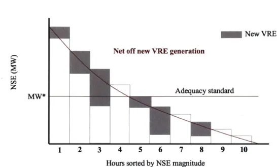
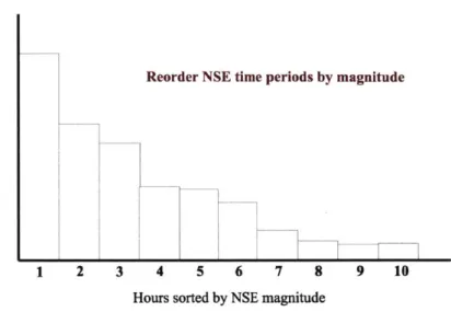
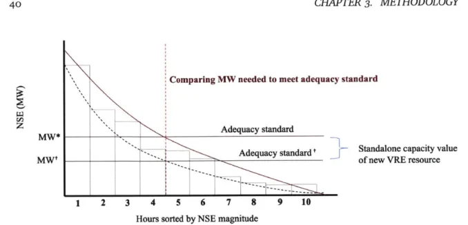
To calculate the standalone capacity value, first determine how much of the added VRE resource's generation occurred in each of the NSE time periods from the simulation and net off this generation from the NSE magnitude. This process is shown in Figures 3-3 to 3-5. Next, the NSE time periods are reordered so that they are again in order from highest magnitude to lowest magnitude, as shown in Figure 3-6. Figure 3-7 shows that the new capacity required to be added to meet the LOLH adequacy standard is MWt. The difference between MW* and

MWt is the standalone capacity value of the added VRE generation, seen in Figure 3-8.

U,

Adequacy standard

1 2 3 4 5 6 7 8 9 10

Hours sorted by NSE magnitude

Figure 3-1: Capacity addition required to achieve LOLH target

Adequacy standard

1 2 3 4 5 6 7 8 9 10

Hours sorted by NSE magnitude

Figure 3-2: Capacity addition required to achieve normalized EUE target

MW*

U,

3.2. STANDALONE CAPACITY VALUE

New VRE generation

Adequacy standard

1 2 3 4 5 6 7 8 9 10

Hours sorted by NSE magnitude

Figure 3-3: Capacity addition required to achieve LOLH target and co-incident VRE generation with

NSE time periods rz~

M4W*

New VRE generation Net off new VRE generation

Adequacy standard MW*

--1 2 3 4 5 6 7 8 9 10

Hours sorted by NSE magnitude

Figure 3-4: VRE generation co-incident with NSE time periods reduces NSE

Net off new VRE generation

1

Hours sorted by NSE magnitude

Figure 3-5: VRE generation netted off of NSE time periods

z

3.2. STANDALONE CAPACITY VALUE

z

z

Reorder NSE time periods by magnitude

1

Hours sorted by NSE magnitude

Figure 3-6: NSE time periods reordered by magnitude

Find new MWI that meets adequacy standard

Adequacy standardt

1 2 3 4 5 6 7 8 9 10

Hours sorted by NSE magnitude

Figure 3-7: New capacity addition required to meet LOLP target MWt

Comparing MW needed to meet adequacy standard

Z _{Adequacy standard}

MW*-T

MW-t Adequacy standard'

Standalone capacity value

of new VRE resource

1 2 3 4 5 6 7 8 9 10

Hours sorted by NSE magnitude

Figure 3-8: Standalone capacity value of added VRE generation

3.3 Integrated capacity value

To calculate the integrated capacity value, the simulations are re-run with the added VRE generation included. This allows other units, principally energy storage resources, to change their operations in response to the new VRE resource. Figure 3-9 shows the MW* of additional capacity necessary to meet the LOLH reliability target in this scenario. The integrated capacity value is the difference between the scenario without VRE and the scenario in which VRE is included in the dispatch simulation, seen via an illustrative example in Figure 3-10. Note that the optimization does not preferentially reduce NSE in hours that are high in NSE over hours that are low in NSE. While the total NSE (the area under the curve) for the integrated case must be less than or equal to that for the standalone case since a constraint has effectively been relaxed, it is possible that there will be individual hours with higher NSE in the integrated case than the standalone case.

3.3. INTEGRATED CAPACITY VALUE

Re-dispatch with new VRE resource

:1

Adequacy standard

1 2 3 4 5 6 7 8 9 10

Hours sorted by NSE magnitude

Figure 3-9: Capacity addition required to achieve LOLP target with new VRE generation included in dispatch simulations

LOLH*

_ Base case

--- Standalone Integrated

175MW due to portfolio effect 125MW standalone value

300 MW integrated value

LOLH

Figure 3-10: Portfolio effect as difference between standalone and integrated capacity values using the LOLH criterion

z

z

3.4

Portfolio effect

The difference between the standalone and integrated capacity values is the portfolio effect. The portfolio effect is the additional capacity value gained by the synergy of VRE and the existing fleet, hypothesized to be principally energy storage resources but also potentially including other units. Figure 3-10 shows a calculation of the portfolio effect in an illustrative example for the LOLH target and Figure 3-11 for the normalized EUE target. In Figure 3-11, each shaded region is equal-area, corresponding to the allowable EUE. All units in the fleet may contribute to the portfolio effect by changing their output in response to the added VRE resource. By fixing the output of energy storage resources and rerunning the integrated case dispatch model, we can isolate their contribution to the portfolio effect. In the case of a capacity market, how to distribute the portfolio capacity value among contributing units in the fleet and the added VRE resource must then be considered. Methods from cooperative game theory such as the Shapley value may be appropriate.

900 825 700 Base --- Stand - Integr

125 MW due to portfolio effect 75 MW standalone value - - - -200 MW inte case ilone ated grated value LOLH

Figure 3-11: Portfolio effect as difference between standalone and integrated capacity values using the normalized EUE criterion

Chapter 4

Dispatch model

4.1

Model description

The capacity value calculation methodologies examined require a least-cost dispatch solution subject to load, VRE resource production, and generator and storage resource constraints. This section describes the economic dispatch model that yields this dispatch solution, developed using a mixed integer programming (MIP) approach. To achieve a runtime reasonable to demonstration of the proposed methodology for capacity value calculations, the model assumes a single balancing area, omitting transmission constraints and nodal analysis. Demand is assumed to be perfectly inelastic. The model uses block loading, an approximation allowing a unit to come online in a single time step to a value between its minimum and maximum operating capacities. The model does not distinguish between cold, warm, and hot states of a unit. Maintenance scheduling and forced outage rates of thermal generators are also omitted in this illustrative model.

The model is written in Julia with options to use either the Gurobi solver or the open-source Compuational Infrastructure for Operations Research Branch and Cut (CBC) solver. The model uses a user-input solution horizon and look-ahead period. For instance, a user may choose to solve for 3 days at a time with a look-ahead period of 1 day, which requires the model to solve for 4 days and discard the last day before stepping forward 3 days. Carry-over parameters for, e.g., unit commitment and ramping constraints, may optionally be used but

are not included here. In this use case, the model is used to run parallel batches of problems without concern for accuracy of total startup costs or solution time horizon edge behavior, provided the solution horizon and look-ahead period are sufficient to adequately simulate unit commitment decisions. General problem formulation was influenced by Byers (2015) and Chang, Tsai, Lai, and Chung (2004). Storage constraints were influenced by Krishnamurthy,

Uckun, Zhou, Thimmapuram, and Botterud (2017), Li, Uckun, Constantinescu, et al. (2016),

and Wankmiller, Thimmapuram, Gallagher, and Botterud (2017). Notation was influenced

primarily by Byers (2015) and Chang et al. (2004).

4.2

Model formulation

4.2.1

Description of variables and parameters

Table 4.1 shows the decision variables and parameters for a simulation over a single horizon and look-ahead period.

Table 4.1: List of dispatch model variables and parameters

Variables

Definitions

Decision variables

Ui = 1 if generator i is on at time t, 0 otherwise

o" = 1 if generator i is turned on at time t, 0 otherwise

Off = 1 if generator i is turned off at time t, 0 otherwise

Pti Committed generation (MW) for generator i at time t

Ptw Generation for wind resource w at time t

Generation for PV resource v at time t