HAL Id: hal-01847521
https://hal.insa-toulouse.fr/hal-01847521
Submitted on 1 Apr 2019HAL is a multi-disciplinary open access archive for the deposit and dissemination of sci-entific research documents, whether they are pub-lished or not. The documents may come from teaching and research institutions in France or abroad, or from public or private research centers.
L’archive ouverte pluridisciplinaire HAL, est destinée au dépôt et à la diffusion de documents scientifiques de niveau recherche, publiés ou non, émanant des établissements d’enseignement et de recherche français ou étrangers, des laboratoires publics ou privés.
The impact of latent heat exchanges on the design of
earth air heat exchangers
Emanuel da Silva Diaz Estrada, Matthieu Labat, Sylvie Lorente, Luiz A. O.
Rocha
To cite this version:
Emanuel da Silva Diaz Estrada, Matthieu Labat, Sylvie Lorente, Luiz A. O. Rocha. The impact of latent heat exchanges on the design of earth air heat exchangers. Applied Thermal Engineering, Elsevier, 2018, 129, pp.306-317. �10.1016/j.applthermaleng.2017.10.007�. �hal-01847521�
1
The impact of latent heat exchanges on the design of Earth Air Heat Exchangers
Emanuel da Silva Diaz Estrada1, Matthieu Labat2, Sylvie Lorente2, Luiz Rocha3
1
C3, Universidade Federal do Rio Grande, Brazil
2
LMDC, INSA/UPS Génie Civil, 135 Avenue de Rangueil, 31077 Toulouse cedex 04 France.
3
Mechanical Engineering Graduate Program, Universidade do Vale do Rio dos Sinos, 93022-000 São Leopoldo, Rio Grande do Sul, Brazil.
Abstract:
The work documents the design of Earth-Air Heat Exchangers based not only on sensible heat
transfer, but also on latent heat exchanges. We compare the impact of the climate of Brazil and south
of France on the relevance of such systems. The duct length is determined in order to obtain
maximum underground heat exchanges. A time dependent model combined to actual weather data is
developed to show when an underground heat exchanger becomes a good option in a tropical
climate. The three-dimensional version of the model accounts for heat transfer in the soil and for heat
and moisture transfer along the underground pipe. The comparison with a 1D model allows to
propose a straightforward approach to assess the cooling/heating potential of different climatic
regions.
Keywords: underground heat exchanger, tropical climate, design
Nomenclature:
Latin Symbols Description Unit
2 cp Specific heat J·kg-1·K-1 D Inner diameter m Dv Mass diffusivity m2.s-1 f Friction factor m2.s-1 h Specific enthalpy kJ·kg-1
hc Convective heat transfer coefficient W·K-1·m-2
hm Convective mass transfer coefficient kg.m-2·s-1
k Thermal conductivity W·m-1·K-1
L Length m
Le Lewis Number -
Lv Latent heat kJ·kg-1
Mass flow rate kg·s-1
Nu Nusselt number -
p Perimeter m
P Pressure Pa
P’ Period hour
Pr Prandtl number -
Heat transfer rate W
ReD Reynolds number -
Sh Sherwood Number -
t time s
T Temperature °C
w Moisture content kgvapor/kgair
Greek Symbols
3 γ
ρ
Inverse of the damping depth
Temperature difference Coefficient (Eq. 5) Density m-1 K - kg·m-3 φ Relative humidity - Subscripts a Air ha Humid air in Inlet sat Saturation v Vapor w Wall
1. Introduction and background
An earth-air heat exchanger (EAHE) consists of one or several ducts buried in the ground, connected
from one end to the outdoor air, and to the other end to the ventilation system of a building. Because
of the high thermal inertia of the soil, the outdoor temperature variations are progressively smoothed
along with the soil depth. Therefore, the ground can be considered as a huge thermal reservoir, which
temperature remains milder and more stable than the outdoor air temperature all over the year. The
air temperature at the pipe outlet is different from the inlet thanks to the heat exchanges occurring
with the soil. This potentially allows reducing the heating or cooling loads at building scale.
Most cases are related to office buildings or typical residential buildings. A considerable number of
4
design stage, the impact of the pipes length, the number of pipes, the cross section of the pipe and the
pipe depth have to be determined in order to enhance the EAHE performances. The latter is of
significance. Most authors advise burying the pipes as deeply as possible in order to take advantage
on the ground thermal inertia. The excavation cost is the sole feature limiting the pipe depth, which
generally remains between 1 and 3 meters. As observed in [7], a deeply buried pipe should indeed be
effective at smoothing yearly temperature variations. However, it may be worth smoothing daily
variations instead, depending on the building loads and on the local climate. This could be easily
achieved by burying pipes less deeply.
Many authors rely on heat transfer calculations to give a comprehensive analysis of the thermal
behavior of EAHE and to improve its design. The methodology differs in terms of complexity and
computational time. For example, the transient heat transfer taking place in the pipe was solved
analytically in [8] under strong assumptions such as undisturbed soil surface temperature. Such an
approach allows to integrate easily the EAHE model in a building simulation tool, as exemplified in
[9,10]. Heat transfer in the ground was be modelled to obtain more realistic results, as in [4,11-13]. A
more refined approach was presented in [11], where a Computational Fluid Dynamic code was used
to model the air transfer in the pipes whereas heat transfer in the ground was modelled up to a depth
of 15m. However because of the high computational time, some simplifications were needed, like by
considering a smaller domain for heat transfer in the soil. A possible alternative is to use model
reduction techniques as presented in [14] in the case of borehole heat exchangers. The drawback of
these techniques is that they are time-consuming and should not be employed for feasibility studies.
The work presented in this paper takes place in the framework of a larger project which intends to
define the potential of EAHE in Brazil. Many EAHE were built over the world during the last
decades, which resulted in a wide range of systems installed under different climates: 18 examples
were reviewed in Santamouris et al. [1], examples of the Mediterranean climate can be found in [1–
5
studied in [11,18,19] (humid), and in [10,20] (dry). Most systems were designed under rather dry
climatic conditions, and humid climates, such as in Brazil, were not studied as intensively. Still, 8
Brazilian climates were compared in [19] and the potential benefits of EAHA was discussed. In the
state of Rio Grande Do Sul, Vaz et al. [18] indicated that the air temperature change from the pipe
entrance to its exit was on an average of 2K. Unlike under a continental climate where the soil
temperature can be, at an equivalent depth, up to 10K lower than the ambient temperature because of
seasonal time-lag, the Brazilian climate does not allow such temperature amplitudes. As a result, the
relevance of EAHE systems is not very clear under Brazilian climatic conditions. One of this study
objectives is to give insight on this issue.
A key feature is that the temperature decrease is not the sole impact of an EAHE in cooling mode;
the system may also influence the air moisture content, and as a consequence the indoor moisture
balance. The indoor relative humidity tends to increase during the night and to decrease during
daytime when using an EAHE. High indoor relative humidity is not desirable as it negatively impacts
indoor air quality [21], enhances fungal and mold growth [3] and may lead to sanitary problems [7].
Regarding energy savings however, the EAHE efficiency can be increased by 25% by mass transfer
in summer conditions, and decreased by 20% in winter conditions in central Europe (Switzerland), as
underlined in [8]. We considered that the influence of moisture transfer on the global performances
of an EAHE is sizeable and worth investigating for the specific case of Brazilian climates.
As underlined in [4,8,22], moisture transfer occurs along the pipe and may significantly influence the
efficiency of the heat exchanger. Condensation may happen if the dew temperature of air at the inlet
is higher than the surface temperature of the pipe. From a technical viewpoint, it means that the pipe
network should be embedded with a slight slope in order to drive the condensed water to a location
where it could be collected and pumped outside the network. This aspect is hardly accounted for in
the modelling or discussed in the result analysis. In a monitored greenhouse equipped with an EAHE
6
evaporation) represented 30% of the global energy balance. A similar ratio was computed in [8], yet
the authors indicated that the latent part of heat transfer was mostly dominated by water infiltrations
in the pipes, rather than condensation or evaporation. The analysis of the numerical results shows
that sensible heat transfer is predominant on the first 10 meters in the pipe, and that latent heat
transfer becomes dominant further.
In this work, we study the energetic potential of an EAHE not only based on sensible heat exchanges
but also on latent heat exchanges. We consider a building where a refrigerating unit is used to
permanently maintain comfortable indoor conditions. The EAHE is used in complement. More
precisely, we intend to find the conditions for which an EAHE system meets the objectives of
reducing the air conditioning needs under a climate such as the one of Brazil. Usually, cooling is
synonymous with decreasing the temperature between the inlet and the outlet of the pipe. As the
basic feature of an EAHE is to pre-cool the air blown into the house in summer, a decrease in the
energy consumption of the refrigeration system is expected. However, moisture condensation
happens almost systematically within a refrigerating unit and accounts for a large part of its energy
consumption. Using an EAHE may not systematically yield to lower the energy consumption of the
refrigerating unit, because of possible moisture increase through the pipe. The refrigerating unit must
remove the excess moisture which increases the overall cooling load. This can be simply illustrated
by considering the psychrometric diagram (Fig 1), which includes both the sensible and the latent
heat through the enthalpy of humid air. Let us assume that the temperature and relative humidity air
at the inlet of the pipe are Tin and RHin respectively. The dew point temperature is denoted by Tdew,
and the humid temperature is denoted by Thumid. If Tw is the temperature of the pipe wall and
assuming a perfect heat exchanger, one can distinguish 3 different configurations, represented by 3
areas in Fig 1:
Configuration A (Tw < Tdew): the moisture content at the outlet is lower than at the inlet,
7 Configuration B (Tdew < Tw < Thumid): the moisture content increased, but the enthalpy of
humid air is reduced, so the cooling load is still diminished.
Configuration C (Thumid < Tw < Tin): the moisture content increased in such a way that the
enthalpy is higher at the outlet, yet the temperature has decreased. Obviously, the EAHE
should not be used in this case.
These cases would be obtained if the wall was completely wet and the pipe was long enough. More
probably, the properties of humid air at the outlet will range between the ones at the inlet (hin) and
the pipe wall (hw). In sum, an EAHE will effectively reduce the cooling loads of a refrigerating unit
as soon as the wall temperature remains below the humid temperature of outdoor air. If the latter is
exceeded, the presence of water inside the pipe will increase the enthalpy, which will make the
EAHE inefficient. Yet latent heat is hardly considered in the design of EAHE.
This paper investigates how an EAHE would perform in a humid climate, and if its use would
effectively lead to energy savings. As Brazil is a country with a wide range of climates, the work is
not limited to one single location. For comparison purposes, the weather conditions of a European
country where it is acknowledged that EAHE systems perform well is also be considered. The study
starts with a simplified approach applied to a rather wide range of Brazilian climate, then the
complexity of the physics is progressively increased while focusing on the regional Brazilian
climates which seem the most promising for an EAHE implementation. The paper is divided as
follows: the next section is dedicated to the definition of the cooling potential of EAHE, based on
simple indicators which can be obtained from general climatic conditions. An analytical model of
EAHE accounting for heat and mass transfer within the pipe in steady state is presented in section 3.
The latter is used to highlight the influence of latent heat transfer in the global EAHE energy
performances and to set the length of the pipe. Next steps consist in the time-dependent modelling of
8
2. Cooling potential
2.1 Thermal characteristics in the French and Brazilian locations
We consider two different countries (Fig. 2): One is Brazil, while the other is France and more
specifically the region of Montpellier. Such locations correspond to the choice of places with
relatively hot temperatures in the summer and different moisture levels. For example, the annual
mean temperature and relative humidity are 23.15°C and 78.3% in Rio do Janeiro, and 14.82°C and
68.7% in Montpellier, while the annual temperature amplitude is 2.73 K for Rio do Janeiro, and 12.1
K for Montpellier.
The soil temperature is obtained from the analytical function [23]:
(1)
where is the soil temperature at time t and depth z, is mean temperature at the soil surface and t0 is the time lag needed for the soil surface temperature to reach . In Eq. (1) Az is the
amplitude of the temperature wave at a depth z, and time t, and decays exponentially with the depth
as follows:
(2)
The inverse of the damping depth, γ, is
(3)
where P’ is the period of the oscillation (1 year here, expressed in hours) and α is the soil thermal
one-9
dimensional and the surface temperature T(0,t) equals the air temperature [24]. The parameters Tm,
and A0 were extracted from weather data provided by the internet databases Energy Plus [25] and
INMET [26]. T(0,t) is obtained by curve fitting the weather data to get the parameters A0 and t0.
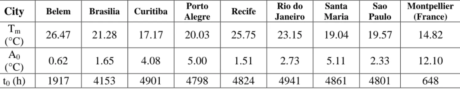
Table 1 shows the values used for each region. The soil thermal diffusivity was chosen identical in
all the cases (α = 0.0023 m2/h in Eq. (3)).
Table 1: Soil function parameters
City Belem Brasilia Curitiba Porto
Alegre Recife Rio do Janeiro Santa Maria Sao Paulo Montpellier (France) Tm (°C) 26.47 21.28 17.17 20.03 25.75 23.15 19.04 19.57 14.82 A0 (°C) 0.62 1.65 4.08 5.00 1.51 2.73 5.11 2.33 12.10 t0 (h) 1917 4153 4901 4798 4824 4941 4861 4801 648
Figure 3 shows the envelope of the extreme temperatures reached by the soil over the year for Rio do
Janeiro and Montpellier. See the large temperature amplitude of the soil temperature in the South of
France relatively to the values measured in Rio.
2.2 First estimation of the potential of EAHE
To give a first estimation of the potential of EAHE for reducing the cooling loads of a
refrigerating unit, we propose to rely on the assumption developed in the introduction: the use of
an EAHE is beneficial if the temperature of the wall of the buried pipe (Tw) is lower than the
humid temperature of outdoor air (Thumid). The latter was computed based on hourly climatic data
(relative humidity and dry bulb temperature). We considered that the pipe was buried at a depth of
about 3 meters following [27]. The pipe wall temperature Tw is assumed to be the soil temperature
at the considered depth, and is calculated based on Eq. (1). Assume is the temperature difference between Thumid and the wall.
10
(4)
A positive value means that the EAHE would help reducing the cooling load. η represents the time
(in %) in the month during which using the EAHE is beneficial.
(5)
Figure 4 allows to identify two different behaviors. η is lower than 5% all over the year in the
regions of Belem, Brasilia and Recife. Higher values of η were obtained for Curitiba, Rio, Porto
Alegre, Santa Maria and Sao Paulo (up to 79% for Curitiba in January). Given the criterion proposed
here (based on the humid temperature), it seems relevant to use an EAHE for these four locations,
yet for a limited period of time only. This result can be linked to the A0 parameter (see Table 1)
which represents the amplitude of the temperature variation over one year at the soil surface: the lowest values of η were obtained for locations with the lowest A0, meaning that the potential of the
EAHE for cooling decreases along with seasonal temperature amplitude. This approach does not give
any information on the energy savings potential. Yet, it clearly exhibits the differences between the
different Brazilian climates. Considering Fig.1 and Fig. 4, the EAHE energy savings potential is
greater in the southern part of the country.
3. Steady state analysis
This section details the heat and mass transfer model developed within the pipe. First, the
steady-state heat and mass balances are presented. This approach allows to determine one of the EAHE
design parameters: the pipe length above which no significant improvement would be observed.
3.1 Analytical model
A conceptual sketch of the earth air heat exchanger (EAHE) is shown in Fig. 5. The system consists
of a fan blowing air into a cylindrical duct. The exact position of the fan does not matter, as long as
11
be accounted for in the energy balance, and may influence the thermal efficiency of the heat
exchanger. For the sake of simplicity, the geometry of the system at the inlet and at the outlet was
not considered in this study; the region of interest is the horizontal part of EAHE of length L and
diameter D.
Consider the elemental volume of thickness dx represented in Fig. 5. We assume that the entire pipe
surface is wet because of water infiltration. For more details on this assumption, see [28]. This is an
extreme case, the opposite case (dry wall) will be considered later. The wall temperature is Tw. Air
enters the pipe at Tin and RHin, with Tin > Tw. If Tw is below the dew point temperature, because the
moisture content of the air at inlet is higher than the wall moisture content, the vapor carried by the
air flow along the duct will condensate.
The mass flow rate of humid air is written , and where is the dry air mass
flow rate and is the vapor mass flow rate. Mass conservation requires
(6)
where represents the condensed water in time along dx.
The energy conservation in steady state writes
(7)
where is the specific enthalpy. Equation (7) can be written as
12
The specific enthalpy of humid air is , where and are
respectively the heat capacity of air and vapor, is the water content, and is the latent heat of evaporation/condensation.
The heat transfer rate has two contributions. The first one is due to sensible heat transfer, while the
second contribution appears because of condensation: . The mass flow rate of condensed water in the elemental domain is given by
(9) where is the duct perimeter, is the mass transfer coefficient, is the humid air density. We have
(10)
where is the convective heat transfer coefficient. Equation (10) can also be expressed as
(11)
where is the Sherwood number, is the vapor diffusivity coefficient, is the Nusselt number, is the Lewis number, and is the humid air specific heat. In configurations such like ours, the ratio is
13 (12) or (13)
Considering that at the pipe inlet (x = 0) , we have
(14)
where for the sake of clarity we wrote , and .
Note that this approach is still valid if Tw exceeds Tin, meaning that is suitable if the EAHE is used
for pre-heating instead of pre-cooling.
3.2 Case studies
As an application, we consider now two case studies: The inlet conditions, representative of a
tropical climate (hot and humid), are Tin = 27°C and RHin = 85%, while they are Tin = 27°C and RHin
= 62% to be close to a continental climate in summer (hot and dry). In the latter, the ground
temperature is 19°C. A ground temperature of 23°C was picked in the first case, both corresponding
to a depth of almost 3 m underground (see Fig. 3) and equal to Tw. In accord with Fig. 1, these two
cases belong to configuration A. Under the drier climate, the wall temperature is nearing the dew
point temperature, while the difference between the two temperatures is more significant for the hot
14
Note that the objective here is not to model actual underground networks but rather to compare the
merit of the EAHE in two very different climatic conditions. To this sake, the pipe diameter was fixed to D = 10 cm and the mass flow rate was chosen to be 40 g/s. Keeping these values in mind, it is now possible to check the assumption that led to Eq. (10). In the case of a duct with a
uniform wall temperature in turbulent flow, the Nusselt number is given by the Dittus and Boelter
correlation [29]
(15)
Here 68.3, and 23 000.
By the same token, the Sherwood number can be obtained by substituting the Prandtl number by the Schmidt number ( )
(16)
Here . Because the Lewis number ( ) is 0.88, the ratio is indeed about 1. The analytical approach proposed so far assumes that the entire wall surface is wet. This is an
extreme case, the opposite one being that the duct surface remains dry. Hence, the total enthalpy
corresponding to such case is calculated by maintaining the latent contribution equal to the inlet
condition. We present in Fig. 6 the evolution of the total enthalpy along the duct in those two cases
as a function of the pipe length in the hot and dry climate (in summer). h1 is the total specific
enthalpy accounting for both sensible and latent heat transfers, while h2 represents the total specific
enthalpy when only sensible exchanges are considered ( ). The results are given in the
non-dimensional form defined in Eq. (14). In this case, the latent heat exchanges are not significant as the
15
Figure 7 shows the results for the humid climatic conditions. The latent heat exchange represents an
important share of the total heat exchange because the difference between the dew point temperature
and the wall temperature is higher. This is important because in most analysis of such EAHE, only
the sensible heat exchanges are accounted for, which may lead to the erroneous conclusion that the
implementation of the underground network is not worthy because of the low temperature decrease.
Cooling potential is not only about temperature decrease but also moisture content reduction. Figure
7 shows that in reality the underground heat exchanger can lower the water content of the air blown
at the exit of the pipe. As already mentioned in the introduction, this would not only lead to energy
savings, but also improve indoor thermal comfort and reduce the risk of mold development indoor.
Finally, Figs. 6 and 7 allow also to estimate the pipe length above which the total enthalpy remains
constant. According to the methodology presented here, this length is between 50 and 60m.
4. Time-dependent problem
First, we present a 3D model accounting for conduction heat transfer in the soil and combined to the
latent and sensible heat exchanges along the pipe. The results obtained with the 3D model are
compared to the results of the unsteady-state version of the model developed in Section 3.1. In the
former the wall temperature is calculated from the heat exchanges between the soil and the air
flowing along the pipe, in the latter Tw is given by Eq. (1) at the depth where the pipe is buried.
4.1 EAHE performances assessment including heat transfer in the soil
We consider a 3D model for the unsteady heat conduction in the soil, combined with a 1D model for
the pipe with an approach equivalent to what was developed in steady state. The soil volume is
parallelepiped of length L (variable), height H, and width W. We chose H = 15m, W = 5m [10]. The
soil thermal diffusivity is identical to the one previously chosen. The pipe of length L (obtained from
16
Fourier’s law of conduction is solved in 3D and non-steady state for the soil, while the presence of
the underground pipe acts as a heat source (or sink) to the ground. The heat emitted by the source (or
received by the sink) is calculated per unit length of pipe, once the energy balance is solved along the
pipe, keeping in mind that the ratio is about 1. The wall temperature needed to determine the wall enthalpy is calculated from the energy balance at the wall, stating that the heat
transfer from the soil is identical to the heat flux inside the pipe.
The energy balance which was defined initially in steady state in Eq. (13), becomes
(17)
which means that in this case, the duct wall is assumed to be wet all along. Here, A is the pipe cross
section. The pipe perimeter which appears in Eq. (17) is the same as in the steady state configuration
(diameter of 10 cm). The mass flow rate is kept at 40 g/s. Equation (17) was implemented in the PDE
(partial differential equations) module of a finite elements numerical code [30].
The boundary conditions are given by Eq. (1) at the soil surface (z = 0). A symmetry condition is
imposed on all the other faces of the soil volume. The air temperature and relative humidity are
provided at the entrance of the pipe from the weather data (Rio do Janeiro or Montpellier). A zero
enthalpy flux condition is chosen at the exit of the pipe. The initial temperature condition for the
entire domain is from Table 1, and the initial moisture content is determined at the same
temperature for a relative humidity of 100%. Mesh refinements were performed until the relative
difference in the total enthalpy at the exit of the pipe between two consecutive refinements was less
than 1.5%, at every time step for a 3 months simulation time.
We show in Figs 9 and 10 the results obtained respectively for the case in France (Montpellier) and
in Brazil (Rio do Janeiro). Here L is 50 m for the French case, and 60 m in the case of Brazil. The
results are given for one full year starting on January 1st, with a time step of 1 hour. Plotted in these
17
both sensible and latent heat transfers (h1) if the pipe wall is wet all along. Plotted also in Figs. 9 and
10 is the relative error made in solving the problem with the 1D model. In this case, we solved Eq.
(17) alone with the same initial conditions in the pipe and the same inlet and outlet boundary
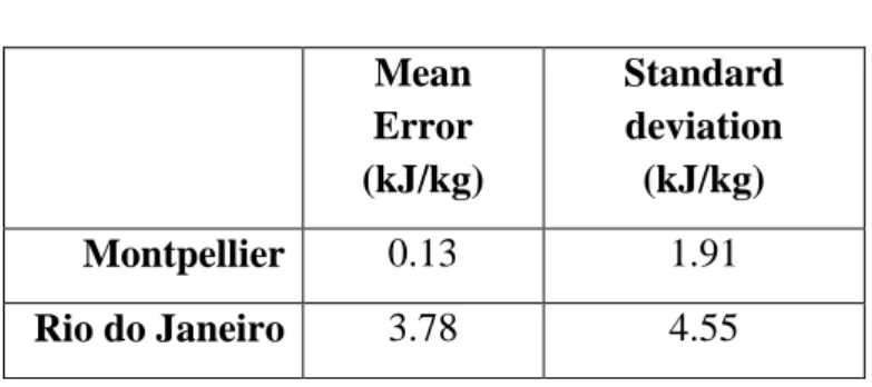
conditions. Eq. (1) was applied to calculate Tw at z = 3m. Table 2 shows the corresponding mean
error and the standard deviation
Table 2: 1D model Mean Error (kJ/kg) Standard deviation (kJ/kg) Montpellier 0.13 1.91 Rio do Janeiro 3.78 4.55
In sum, the 1D approach follows with a reasonable accuracy the enthalpies evolutions in time
predicted by the 3D approach.
4.2 EAHE performances by using an analytical model for the wall temperature
The 1D approach is pursued to assess the cooling/heating potential of different regions in Brazil.
Note that this approach is complementary to the one proposed in Section 2 and plotted in Fig. 4,
considering the enthalpy instead of the temperature. It gives information not only on the period when
the EAHE is relevant for cooling but also on the heat transfer intensity. Moreover the influence of
the pipe length can easily be studied.
The 1D model was run with several tube lengths: L= 20m, and 30m, together with the length
obtained from the steady state analysis. Plotted in Figs. 11 and 12 are the enthalpy changes over the
course of 1 year when sensible and latent heat exchanges are considered (h1), and when only the
sensible enthalpy exchange is accounted for, the latent enthalpy being kept at its entrance value (h2).
In the latter, the EAHE length is L = 50 m for the France case (Montpellier), and 60 m for Brazil
18
compared to the other Brazilian climates. The values presented in Figs. 11 and 12 are the inlet and
outlet enthalpies, together with the wall enthalpy, which is considered constant along the pipe. Recall
that this means that at every time step the moisture content is w(L) to calculate h1(L) whereas it is win
for h2(L). From the h1(L) curves we can see the effect of the tube length on the outlet total enthalpies:
they become controlled by the wall conditions when the pipe length approaches the value obtained
with the steady-state assumption. This latest result shows that the steady-state approach is relevant
for determining the maximal length of the EAHE. Figures 11 and 12 represent actually the envelope
between the two extreme cases.
To ease the analysis of the results presented in Figs. 11 and 12, the potential of heating and cooling
was determined by plotting the monthly average difference between the enthalpy at the heat
exchanger outlet and its inlet. Plotted are the total enthalpy differences together with the sensible
ones. Figures 13 and 14 correspond respectively to Montpellier and Rio do Janeiro.
During the fall and winter in France (Figs. 11 and 13), the global trend of the enthalpy demonstrates
the heating potential of the underground, as the enthalpy at the exit is higher than the one at the inlet.
Moreover, a difference is noticed when latent heat transfer is accounted for, as the system can benefit
from latent heat exchanges. From May to August, we see that that the results are very close on an
average, meaning that the latent heat exchanges are not significant. Still, the ground cooling potential
is clearly highlighted. The impact of latent exchanges is critical during the mid-season which
corresponds to the months of April and September. Accounting only for sensible heat transfer, the air
blown from the buried pipe would be considered as able to cool.
The trends exhibited in the case of Rio (Figs. 12 and 14) are drastically different. If the pipe is dry,
the air at the exit of the duct has a specific enthalpy (h2) lower than at the entrance during half of the
year. It is the opposite when accounting for the latent heat exchanges along the pipe, except
punctually in the very beginning of the Brazilian summer (November, see Fig. 12). The variability of
19
enthalpy can be decreased but the latent enthalpy is increased. Even though the EAHE can slightly
impact the sensible enthalpy of the air blown into the building in the case of the tropical climate, Fig.
14 (Rio) shows that the latent enthalpy is always increased. The direct consequence is that the power
of the air conditioning system needed in the building must be increased in order to dehumidify the
indoor air, leading to the exact opposite expected result.
What should be the conditions for which an EAHE system meets the objectives of reducing the air
conditioning needs under a climate such as the one of Brazil? Based on this idea, we looked for
conditions that would correspond to the methodology proposed in Fig. 1. The region around Porto
Alegre seems to be a good candidate. The mean annual temperature and relative humidity are 20°C
and 74%, the annual temperature amplitude is 5K, as indicated in Table 1. The cooling and heating
monthly potentials were plotted in Fig. 15. The results show that the EAHE allows to precool during
summer (December and January) the blown air, even when accounting for the latent heat exchanges.
Note that the decrease in enthalpy is lower for Montpellier (Fig. 13), yet the magnitude is of the same
order.
5. Concluding remarks
Earth-Air heat exchangers are an old technique known since the Roman empire around the
Mediterranean Sea. Today, with the increasing concern in global warming and the objective of
including renewable energy in the heating/cooling solutions for indoor comfort, EAHE experiences a
renewed interest in several countries including Brazil. In this work we developed a model to account
for latent and sensible heat exchanges between the buried pipe and the soil. By comparing the results
to the climate of south of France, we look for the conditions when EAHE is an interesting solution.
An example of tropical climate (Rio do Janeiro) was picked and the heat exchanges were envisaged
in 2 extreme cases: considering sensible enthalpy only and adding latent heat exchanges when the
20
may have: Even though in summer the air is blown into the house at a lower temperature than the
outdoor; the air is humidified to such an extent that the air conditioning system would have to spend
more power to maintain indoor comfort.
The 3D modelling of conduction heat transfer through the soil showed almost no difference with the
approach consisting in calculating the pipe wall temperature at its buried depth from an analytical
soil temperature function. The next step of this work will consist in including to the present study the
hydric state of the soil and modelling its impact on the overall heat transfer through the pipe.
Acknowledgments
The authors would like to thank the CAPES-COFECUB program (Ph 854-15) at the origin of this
work. E. Estrada’s one year visit in Toulouse was funded by CAPES, Brazil.
We would like to express our special thanks to Prof. Joaquim Vaz, Federal University of Rio Grande
(Brazil), for his interest in this work.
References
[1] Santamouris M, Mihalakakou G, Balaras CA, Argiriou A, Asimakopoulos D, Vallindras M. Use of buried pipes for energy conservation in cooling of agricultural greenhouses. Sol Energy 1995;55:111–24. doi:10.1016/0038-092X(95)00028-P.
[2] Santamouris M, Mihalakakou G, Balaras CA, Lewis JO, Vallindras M, Argiriou A. Energy conservation in greenhouses with buried pipes. Energy 1996;21:353–60. doi:10.1016/0360-5442(95)00121-2.
[3] Boulard T, Razafinjohany E, Baille A. Heat and water vapour transfer in a greenhouse with an underground heat storage system part I. Experimental results. Agric For Meteorol 1989;45:175– 84. doi:10.1016/0168-1923(89)90042-7.
[4] Boulard T, Razafinjohany E, Baille A. Heat and water vapour transfer in a greenhouse with an underground heat storage system part II. Model. Agric For Meteorol 1989;45:185–94.
doi:10.1016/0168-1923(89)90043-9.
[5] Kassem AS. Energy and water management in evaporitive cooling systems in Saudi Arabia. Resour Conserv Recycl 1994;12:135–46. doi:10.1016/0921-3449(94)90002-7.
21
[7] Hollmuller P, Lachal B. Air–soil heat exchangers for heating and cooling of buildings: Design guidelines, potentials and constraints, system integration and global energy balance. Appl Energy 2014;119:476–87. doi:10.1016/j.apenergy.2014.01.042.
[8] Hollmuller P, Lachal B. Cooling and preheating with buried pipe systems: monitoring, simulation and economic aspects. Energy Build 2001;33:509–18. doi:10.1016/S0378-7788(00)00105-5.
[9] Ascione F, Bellia L, Minichiello F. Earth-to-air heat exchangers for Italian climates. Renew Energy 2011;36:2177–88. doi:10.1016/j.renene.2011.01.013.
[10] Al-Ajmi F, Loveday DL, Hanby VI. The cooling potential of earth–air heat exchangers for domestic buildings in a desert climate. Build Environ 2006;41:235–44.
doi:10.1016/j.buildenv.2005.01.027.
[11] Brum R da S, Vaz J, Rocha LAO, dos Santos ED, Isoldi LA. A new computational modeling to predict the behavior of Earth-Air Heat Exchangers. Energy Build 2013;64:395–402.
doi:10.1016/j.enbuild.2013.05.032.
[12] Mihalakakou G, Santamouris M, Asimakopoulos D. Modelling the thermal performance of earth-to-air heat exchangers. Sol Energy 1994;53:301–5. doi:10.1016/0038-092X(94)90636-X. [13] Vaz J, Sattler MA, dos Santos ED, Isoldi LA. Experimental and numerical analysis of an earth–
air heat exchanger. Energy Build 2011;43:2476–82. doi:10.1016/j.enbuild.2011.06.003. [14] Kim E-J, Roux J-J, Rusaouen G, Kuznik F. Numerical modelling of geothermal vertical heat
exchangers for the short time analysis using the state model size reduction technique. Appl Therm Eng 2010;30:706–14. doi:10.1016/j.applthermaleng.2009.11.019.
[15] Pfafferott J. Evaluation of earth-to-air heat exchangers with a standardised method to calculate energy efficiency. Energy Build 2003;35:971–83. doi:10.1016/S0378-7788(03)00055-0. [16] Serres L, Trombe A, Conilh JH. Study of coupled energy saving systems sensitivity factor
analysis. Build Environ 1997;32:137–48. doi:10.1016/S0360-1323(96)00039-X.
[17] Paludetto D, Lorente S, Modeling the heat exchanges between a datacenter and neighboring buildings through an underground loop. Ren. Energy 2016;93:502-509.
doi.org/10.1016/j.renene.2016.02.081
[18] Vaz J, Sattler MA, Brum R da S, dos Santos ED, Isoldi LA. An experimental study on the use of Earth-Air Heat Exchangers (EAHE). Energy Build 2014;72:122–31.
doi:10.1016/j.enbuild.2013.12.009.
[19] Alves ABM, Schmid AL. Cooling and heating potential of underground soil according to depth and soil surface treatment in the Brazilian climatic regions. Energy Build 2015;90:41–50. doi:10.1016/j.enbuild.2014.12.025.
[20] Ozgener O, Ozgener L, Goswami DY. Experimental prediction of total thermal resistance of a closed loop EAHE for greenhouse cooling system. Int Commun Heat Mass Transf
2011;38:711–6. doi:10.1016/j.icheatmasstransfer.2011.03.009.
[21] Wolkoff P, Kjaergaard SK. The dichotomy of relative humidity on indoor air quality. Environ Int 2007;33:850–7. doi:10.1016/j.envint.2007.04.004.
[22] Soontornchainacksaeng T. Experimental and numerical study of the thermal behaviour of an Earth to Air heat exchanger designed for dwellings. INSA de Toulouse, 1993.
[23] Ozgener O, Ozgener L, Tester JW. A practical approach to predict soil temperature variations for geothermal (ground) heat exchangers applications. Int J Heat Mass Transf 2013;62:473–80. doi:10.1016/j.ijheatmasstransfer.2013.03.031.
22
[24] Hillel D. Introduction to soil physics. New York: Academic Press; 1982.
[25] Weather Data | EnergyPlus n.d. https://energyplus.net/weather (accessed May 27, 2016).
[26] :: INMET - Instituto Nacional de Meteorologia :: n.d. http://www.inmet.gov.br/portal/ (accessed August 10, 2016).
[27] Kepes Rodrigues M, da Silva Brum R, Vaz J, Oliveira Rocha LA, Domingues dos Santos E, Isoldi LA. Numerical investigation about the improvement of the thermal potential of an Earth-Air Heat Exchanger (EAHE) employing the Constructal Design method. Renew Energy 2015;80:538–51. doi:10.1016/j.renene.2015.02.041.
[28] Fan J, Ostergaard KT, Guyot A, Fujiwara S, Lockington DA. Estimating groundwater evapotranspiration by a subtropical pine plantation using diurnal water table fluctuations: Implications from night-time water use. J Hydrol 2016;542:679–85.
doi:10.1016/j.jhydrol.2016.09.040.
[29] Dittus FW, Boelter LMK. Heat transfer in automobile radiators of the tubular type. Int Commun Heat Mass Transf 1985;12:3–22. doi:10.1016/0735-1933(85)90003-X.
23
Figure captions
Figure 1 Identification of three areas in the psychrometric diagram for enthalpy variation in an
EAHE for cooling.
Figure 2 Montpellier (France) and Brazil (the latter is from Ref. 12).
Figure 3 Minimum and maximum soil temperatures for Montpellier (France) and Rio do
Janeiro (Brazil).
Figure 4 Estimation of η for Brazilian climates
Figure 5 EAHE system and model domain
Figure 6 Evolution of enthalpy in a continental climate zone.
Figure 7 Evolution of enthalpy in a tropical climate zone.
Figure 8 3D domain for the numerical simulations.
Figure 9 Difference between inlet and outlet enthalpies in the 3D case and in the 1D case, and
relative error in the Montpellier (France) configuration.
Figure 10 Difference between inlet and outlet enthalpies in the 3D case and in the 1D case, and
relative error in the Rio do Janeiro (Brazil) configuration.
Figure 11 Envelope of the enthalpy at the exit of the pipe, during one year in the case of
Montpellier, France.
Figure 12 Envelope of the enthalpy at the exit of the pipe, during one year in the case of Rio do
Janeiro, Brazil.
Figure 13 Cooling and heating potential in the case of Montpellier, France.
Figure 14 Cooling and heating potential in the case of Rio do Janeiro, Brazil.