Developement of a model for the near-exit plume
of a Hall thruster
by
Felix Ignacio Parra Diaz
Submitted to the Department of Aeronautics and Astronautics
in partial fulfillment of the requirements for the degree of
Master of Science in Aeronautics and Astronautics
at the
MASSACHUSETTS INSTITUTE OF TECHNOLOGY
January'2007
©
Massachusetts Institute of Technology 2007. All
Author ...
Department of Aenautics
rights reserved.
and Astronautics
January 31, 2007
()
Certified
by...
Manuel Martinez-Sainchez
Professor of Aeronautics and Astronautics
Thesis Supervisor
I) DI1
Accepted by ...
....
.. ....
...
.
.
. .
. .
.
.Peraire
Professor of Aeronautics and Astronautics
Chair, Committee on Graduate Students
?MS$ACHUSE1TB INSTMTUE OF TECHNOLOGY
MAR
2
8
2007
Developement of a model for the near-exit plume of a Hall
thruster
by
Felix Ignacio Parra Diaz
Submitted to the Department of Aeronautics and Astronautics on January 31, 2007, in partial fulfillment of the
requirements for the degree of
Master of Science in Aeronautics and Astronautics
Abstract
This thesis presents a fluid model for electron behavior in the near-exit plume of a Hall thruster. The model provides 3D results and allows to study the azimuthal asymmetry induced by the hollow cathode. The model is composed by the charge and energy conservation equations and is intended to solve for the electrostatic potential and the electron temperature. It relies on the results of an external model for the ion behavior. The fluid equations are diffusive and are justified in the limit of small elec-tron Larmor radius. They include the Hall transport, which is usually ignored in 2D approaches due to symmetry. The transport along magnetic field lines is high enough to convert the 3D problem into a 2D problem, where only the directions perpendicular to the magnetic field matter. In such a 2D formulation, the basic structure of the solu-tion for the potential is studied analytically, with the result that the lines of constant potential can be approximately predicted. The potential can be found numerically after transforming the charge conservation equation into a convective-diffusive equa-tion. The numerical results agree approximately with analytical predictions. The results suggest that the asymmetry induced by the hollow cathode mainly depend on how much the cathode perturbs the plasma density distribution.
Thesis Supervisor: Manuel Martinez-Sainchez Title: Professor of Aeronautics and Astronautics
Acknowledgments
I will never be able to thank enough my wife Violeta, my parents, Nieves and Ignacio, and my brother Braulio for their unconditional support. Violeta stood by my side on the good and on the bad days, and let me rob time from our common life. Her calm and lucid personality helped to keep things in perspective, and her warm love made all the long hours bearable. She, more than anything, is the foundation of this thesis. My mother understood my fears and managed to encourage me from the other side of the ocean. Her constant worries were a relief for me because they made me realize that, no matter what, she is the person I can count on. My father always had a calm and wise word, and was the support I needed when I thought I could not go on. My brother Braulio, even though he is a quiet person, let me know how much he believed in me when I was not feeling up to the task.
I also want to thank two excellent friends: Luis and Murat. Luis has been a loyal support, always confident on my abilities. His respect towards my work encouraged me because he is all I can expect to be one day. Examples like Luis make graduate school worth every hour. Murat took the place of the family I had to leave behind, specially my first year. His interest and curiosity led me to question an important part of what I knew; his answers to my doubts were always insightful and helpful.
Thanks to my office mates, Justin and Tanya. We had fun, and we survived together the sour times. This thesis owes a lot to them, too.
I would like to mention the contribution of Manuel. His influence in my work is too large to list here. Enough to say that this thesis would not be possible without his collaboration.
Last, but not least, thanks to Zoltan Spakovszky and Peter Catto, because without them, I would have not been able to stay at MIT, working on this thesis.
Contents
1 Introduction
1.1 Electric propulsion plume studies . . . .
1.2 Near-exit plume model for Hall thrusters 1.2.1 Hall thruster physics . . . . 1.2.2 Hall thruster modelling . . . .
1.2.3 Objectives of the model...
2 Electron fluid model
2.1 Electron equations . . . . 2.1.1 Charge conservation . . . . 2.1.2 Momentum conservation . . . . 2.1.3 Energy conservation . . . . 2.1.4 Sum m ary . . . . 2.2 Solution behavior . . . .
2.3 2D solution: integration along the lines . . . . 2.3.1 Integration of a divergence along the magnetic lines
2.3.2 Charge conservation in the new variables . . . .
2.3.3 Energy equation in the new variables . . . . 2.3.4 General considerations about the 2D equations . . . 2.4 Structure of the 2D solution . . . . 2.4.1 Including the energy equation . . . .
2.5 C onclusions . . . . 9 . . . . 9 . . . . 10 . . . . 10 . . . . 12 . . . . 13 15 . . . . . 16 . . . . . 16 . . . . . 17 . . . . . 19 . . . . . 22 . . . . . 22 . . . . . 24 . . . . . 26 . . . . . 28 . . . . . 30 . . . . . 32 . . . . . 34 . . . . . 41 . . . . . 42
3 3D potential distribution
3.1 Flow-Condition-Based Interpolation (FCBI) Finite Elements
3.1.1 Boundary conditions . . . .
3.2 First approximation to the 3D problem . . . . 3.2.1 Plasma density and ion current density profiles . . . 3.2.2 Magnetic coordinates . . . .
3.2.3 Diffusion coefficients . . . . 3.2.4 Boundary conditions for the thermalized potential . .
3.3 R esults . . . . 3.3.1 Effect of the cathode ion flow . . . . 3.4 C onclusions . . . .
4 Conclusions and Future Work
4.1 Conclusions ... ...
4.2 Future w ork . . . .
A Useful vectorial relations for variable changes
45 . . . . 45 . . . . 49 . . . . 50 . . . . 50 . . . . 56 . . . . 56 . . . . 58 . . . . 61 . . . . 65 . . . . 68 69 69 70 73
List of Figures
1-1 Sketch of a Hall thruster. . . . . 10
2-1 Near-exit plume diagram. The cathode induces a highly asymmetric profile. Due to the fast diffusion along the magnetic field lines, its effect extends far. . . . . 16
2-2 Magnetic coordinates A, and A2 in an axisymmetric, meridional
mag-netic field . . . . 25 2-3 Wall energy losses for a typical ceramic wall at different Te. The plasma
density is fixed at ne = 1017 M-3. . . . . 33
2-4 Hall thruster representation in a A1 - A2 plane. UH = const. lines are
plotted . . . . . 37 2-5 Coordinate system tangent to the boundaries. Note that the direction
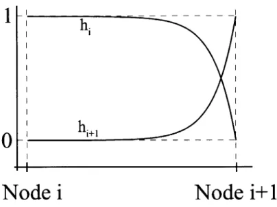
of UH = cOnSt. lines is given by angle a. . . . . 38 3-1 FCBI shape functions in a 1D mesh. . . . . 46
3-2 Galerkin-Petrov method. The Finite Volume is shown in dashed lines.
The interpolation used for computing the flow across the left panel is shown in (a). The interpolation used for the flow across the bottom panel is shown in (b). . . . . 48
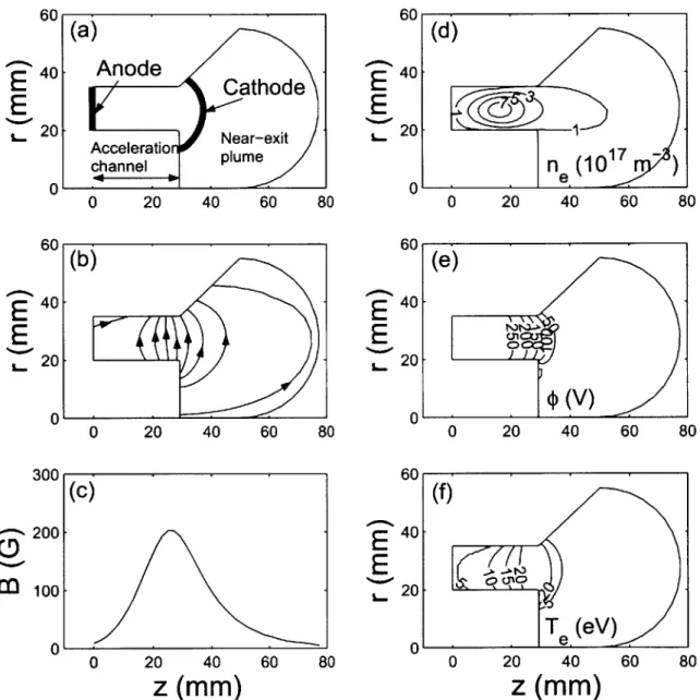
3-3 HPHall results for an SPT-70 thruster. (a) Geometry. (b) Magnetic field lines. (c) Magnetic field strength at r = 27.5 mm. (d) Plasma
density distribution. (e) Electrostatic potential. (f) Electron temper-ature. ... ... 52
3-5 Plasma density in different meridional planes. . . . . 55 3-6 Distribution of A. . . . . 56 3-7 Cathode position and YH distribution in the A - 0 plane. . . . . 59 3-8 Boundary conditions in the 3D physical space and in the A - 0 plane. 60 3-9 * distribution in the A - 6 plane. . . . . 61 3-10 * distribution near the hollow cathode. . . . . 62 3-11
#
distribution in different z = const. planes. The contour lines areseparated by 20 V. . . . . 63 3-12 Current across surfaces A = const. . . . . 64
3-13 0* distribution in a meridional slice that cuts through the cathode. 65
3-14 Potential distribution at the exit of the acceleration chamber (z =
29 mm) for different ionized fractions of the cathode mass flow. The
contour lines are separated by 20 V. . . . . 66 3-15 UH and potential distribution in the A -0 plane for two ionized fractions
Chapter 1
Introduction
1.1
Electric propulsion plume studies
A multiplicity of plume codes based on hybrid simulation have been developed by
many researchers [1, 2, 3, 4]. As these codes mature and comparisons are attempted to lab or space plume data, it becomes evident that one of the essential ingredients is the distributions of density, velocity and temperature of the ions at the initial plane, which is either the thruster exit plane, or a plane chosen some short distance downstream from the exit. Our work intends to improve present models for initial plane distributions in Hall thrusters by solving accurately the near-exit zone.
The near-exit plume is characterized by different aspects that are not covered in the usual plume models:
" Strong magnetic field. " Ionization.
* 3D effects in the electron population induced by the hollow cathode.
Such effects are dealt with in all the two-dimensional (axisymmetric) models that refer to the acceleration channel and a simplified near-exit plume [5, 6, 7]. Therefore, the approach of this work is extending the existing successful models for the plasma
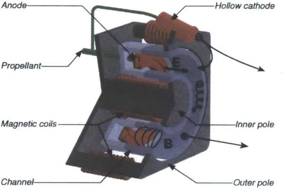
Hollow cathode
Inner pole
Outer pole
Figure 1-1: Sketch of a Hall thruster.
discharge inside the thruster to the near-exit plume, mainly in what is related to the
3D effects.
1.2
Near-exit plume model for Hall thrusters
In this section, the basics of Hall thruster modelling are covered. This brief synthesis of previous research intends to contextualize the present work and to narrow its objectives to the main difficulties in the modelling of the near-exit plume.
1.2.1
Hall thruster physics
The typical geometry of a Hall thruster is shown in figure 1-1. There are other possible shapes, but the most common is the cylindrical acceleration channel, which is shown in the figure. The acceleration channel is usually made of a dielectric ceramic (Boron Nitride is a common choice).
Propellant
Magnetic coils
Channel-A Hall thruster works by accelerating the plasma inside the acceleration channel
through a potential drop. The potential drop is maintained between the anode, at the end of the channel, and the exterior hollow cathode. Both the anode and the cathode are sketched in figure 1-1. The plasma is created by ionizing a neutral gas with low ionization energy cost, like Xenon. The gas is injected through injectors in the anode.
An almost axisymmetric magnetic field is induced by several magnetic poles. This axisymmetric magnetic field (shown in figure 1-1) confines the electrons in the accel-eration channel in order to make the ionization more efficient. The magnetic field is strong enough to confine electrons, but not so strong that it may affect the ions. Thus, the ion Larmor radius is large compared to the size of the thruster and the electron Larmor radius is small. The motion of the ions is just due to the acceleration in the potential drop.
The dynamics of both charged species, electron and ions, are very different. Ions are unmagnetized, and drop through the potential difference, getting accelerated. Most of the ions are created at the same potential (it will be shown in chapter 3). Thus, the ions are almost all at the same speed. They can be considered as a beam. The typical ion energy in these thrusters is on the order of hundreds of volts (the potential difference between anode and cathode), while the ion temperatures found are close to the electronvolt.
The electrons are completly magnetized. Electrons come out of the hollow cathode and fall towards the anode in the potential drop. The magnetic field created by the external poles is high enough to confine them; therefore, the electrons move with the
E x B drift. This drift is pointing in the azimuthal direction almost everywhere, because except for the hollow cathode, the thruster is axisymmetric and the electric field and magnetic field have the directions sketched in figure 1-1. Thus, the electrons can only reach the anode by collisions, since the drift does not lead them to it. The path of a electron is much longer than the size of the thruster because it will turn around the thruster several times before collisions move it towards the anode (the pressure is low enough so that the mean free path is large compared with the
size of the thruster). Actually, collisions are negligible in most of the thruster, and turbulence seems to be the main transport mechanism for the electrons [8, 9, 6].
1.2.2
Hall thruster modelling
There have been three different approaches for modelling Hall thrusters: fully fluid
[10, 11], fully kinetic [7] and hybrid fluid-kinetic [5, 6]. Fully kinetic codes use Particle-In-Cell (PIC) schemes. They contain the most physics, but they are costly and also noisy. Fully fluid models, on the other hand, present their own numerical problems (the ions are hypersonic) and are not justified, specially for the ions and the neutrals: the arguments of short mean free path or small Larmor radius do not apply for them.
Hybrid fluid-kinetic codes, on the other hand, are not as costly as fully kinetic models and can deal with ions and neutrals in a more complete way. The idea is that ions and neutrals must be treated kinetically (usually a PIC code, with maybe some MonteCarlo collisions) whereas electrons, which have a small Larmor radius, can be considered as a continuum. This model can be very accurate, but it depends a lot on the assumption for the behavior along the magnetic field lines. Several different important issues related to the dynamics along the magnetic field lines have been already identified. Almost all of them are related to the plasma-wall interaction: non-Maxwellian distribution functions, high energy electrons coming from secondary emission and backscattering at the wall, etc. These problems have been approached
by PIC simulation [12] and analytically [13, 14].
Even if these kinetic effects are not included in the models, the results are reason-able, with a much lower noise level. The computational time is shorter than for fully PIC codes.
It is important to point out that the models for far plume do not have to worry about the magnetic field because it is too low. That changes the whole approach. However, the near-exit plume discharge characteristics are closer to the features of the plasma in the acceleration channel and, therefore, it is interesting to review the models for Hall thrusters, and not those for far plume.
1.2.3
Objectives of the model
The present thesis is intended to propose a satisfactory approach for a model of the near-exit plume in Hall thrusters. The near-exit plume is specially difficult to model because the cathode induces a axial asymmetry and the problem becomes 3D. All the models mentioned in the previous section are either 1D or 2D, and all of them assume axisymmetry. Now, a 3D study of a Hall thruster is the first step to understand the near-exit plume.
As a first approach, an electron fluid model for a 3D problem will be developed. This is the main difference with previous models, because new physics come into play (Hall transport). A PIC scheme is easy to generalize to a 3D geometry, considering that the magnetic field is not important.
Thus, the main objective is to develop the simplest possible model for fluid elec-trons. Once this is obtained, the PIC model for ions and electrons should be added. This will provide a complete 3D model for the Hall thruster, including the near-exit plume. It will have the advantage of being fast to run (which is important since a dimension has been added) and it will contain most of the physics.
Adding collisions, more complete models for the electron distribution function and other features will allow to understand the relation between the cathode position and the performance of the thruster, the effect of charge exchange collisions in plume divergence, etc.
Chapter 2
Electron fluid model
This chapter is devoted to the presentation and analytical study of an electron fluid model valid for the near-exit plume.
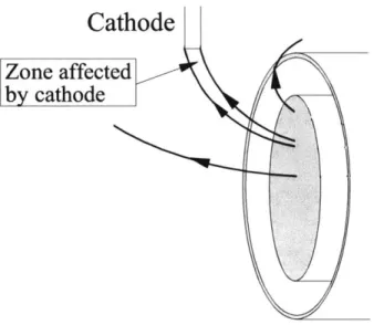
Figure 2-1 presents the typical geometry in the near-exit plume. Even though the geometry of the acceleration channel and the magnetic field is axisymmetric, the cathode induces asymmetry. The diffusion along the magnetic lines is much larger than the perpendicular diffusion. Thus, the effect of the cathode extends really far along the magnetic field lines. This effect and its range are difficult to model because the transport across the magnetic lines has two components very different in nature and value: the Hall transport, perpendicular to the gradients of plasma magnitudes, such as pressure, potential..., and the collisional perpendicular transport. The Hall transport is closely related to the E x B drift and it is connatural to the Larmor motion. The collisional perpendicular transport, much smaller in size, has to do with perturbations on the Larmor motion, such as collisions or turbulence. Note that in the axisymmetric models, the Hall transport lays in the azimuthal direction, balancing out. However, in a 3D case, such as this one, this transport has to be taken into account because it is the most important contribution in the direction perpendicular to the magnetic field.
In what follows we discuss the electron fluid equations and the special mathemat-ical difficulties that appear as a consequence of the combination of strong magneti-zation and three-dimensionality.
Cathode
Zone affected by cathodeFigure 2-1: Near-exit plume diagram. The cathode induces a highly asymmetric profile. Due to the fast diffusion along the magnetic field lines, its effect extends far.
2.1
Electron equations
Electrons are modelled as a continuum. The equations to be solved are charge, momentum and energy conservation.
Since the Larmor radius is really small compared to the typical length in the problem, a simple diffusive model is proposed for all these equations. Such an ap-proximation is acceptable for the motion perpendicular to the magnetic field lines, but it is not as correct along the lines. However, the proposed model is expected to yield results that contain most of the physics.
In the next subsections, the different equations are described and explained briefly.
2.1.1
Charge conservation
Assuming quasineutrality:
V -jj + V -je = 0 (2.1)
ji
is the ion current density, and it is obtained in the ion submodel.j,
= -eneve is the electron current density. It is one of the unknowns that must be obtained fromthe electron equations.
2.1.2
Momentum conservation
In the diffusive limit:
1 ern 1 1
0 = - V(neTe) + V + -Weje X
b
+ Veje (2.2)me me e e
where
#
is the electrostatic potential, T the electron temperature, we = eB/me is the gyrofrequency, b = B/B is the unit vector in the same direction as the magnetic field and ve is a frequency that measures the collisionality and turbulence.je can be solved from this equation:
je jeb -+ jeH + jeL, (2.3)
where
n. Te
Jeb -Urbb
[vq*
+1
(Inno
- I)V
]
(2.4) V + ne TjeH = -- H X
v*
+ In 1 V e) (2.5)no e
ne Te
jel = -- 1
vi#*
+ (ino - I) V1
(2.6)V1 = V -
b
- V is the gradient in the perpendicular direction to the magneticfield.
jeb is the current along the magnetic field line. jeH is the Hall component of the current. It contains the electron current due to the E x B drift, plus the curvature and VB drifts. jeL is the collisional perpendicular current. It accounts for collisions and turbulence.
It is important to point out that in axisymmetric cases, jeH is aimed in the az-imuthal direction, therefore cancelling exactly. Thus, it is not usually included in 2D models.
In these equations, the 'thermalized potential', q* is used. It is defined as:
= - In n (2.7)
e no
no is a constant that can have any positive value. It will be convenient to choose no as the maximum plasma density in the domain. Then, ln(ne/no) will be always negative and of order unity.
The conductivity for the plasma is different in the different spatial directions. In equations (2.4), (2.5) and (2.6), these conductivities are called Ob, GrH and u1:
e2 UD-e 2 e(28 Or = (2.8) meve e2 me We + Ve2 e 2 e Ve L = 2 2(2.10) me We + Ve
Considering that Ve < We near the exit:
Ob > H > 01 (2.11)
The ratio between these different conductivities is the Hall parameter, O3H
We/Ve.
For example, cb/H 1 OH, or UH/U 1 -
/-This means that the plasma tends to homogenize much faster along the magnetic lines, where cb is the conductivity. Then, along the magnetic lines:
b-VO* + In n 1 V ~ 0 (2.12)
(no e
Actually, from the energy equation, we will obtain that W VTe ~ 0, which means that (2.12) is:
b -V#* ~ 0 (2.13)
becomes indeterminate. It can be solved for together with 0* and Te. Plugging equation (2.3) into (2.1):
-V.-
(bOrHi X VO*) - V.- (U1ViqS*)--V - (7H X V(Te/e)) - V - (7VL(Tle/)) + V -ji + V -(bjeb) = 0 (2.14)
yj = cg (in -
),where
, j = H, I.It is important to note that in this equation there are terms of very different order of magnitude. The terms that contain gH and YH are larger by a factor we/ve,
provided the other factors in them are comparable to those in other terms.
Note that Jeb appears in the equation, and it is unknown. To deal with it, an integration along tubes defined by the magnetic field lines will be performed. This integration will eliminate the term that depends on Jeb and leave an equation only with 0* and T as unknowns.
2.1.3
Energy conservation
The energy conservation is given by:
(3neTe) + V - (-je + ge) = -je - V# - neviajiE (2.15)
ot 2 2 e
where q, is the electron heat conduction flux, and neviajEj are the ionization losses. The model for ionization losses is the same used by Fife [5].
The heat conduction can be obtained using a diffusive approximation, similar to the one used to obtain the electron current density (2.3):
qe = qebb + qeH + qe- (2.16)
where
qeb = -bb- VTe (2.17)
(2.19)
Thermal conductivity is highly anisotropic. The values of the different coefficients are: 5 nT, 2 meve 5 neTe We = 2 me w2
+
v2 5 neTe Pe 2me W + Ve (2.20) (2.21) (2.22)For we
>
ve, the coefficients have really different orders of magnitude:Kb >> KH >> KLI (2.23) As it happened with the electrical conductivities, the ratio between the different thermal conductivities is the Hall parameter.
Thermal diffusion is high in the direction of the magnetic field. That means that, as a first approximation, the temperature is constant along the lines:
b - VTe ~ 0 (2.24) Even though b VTe is almost zero, qeb is not zero. By using (2.24), qeb becomes indeterminate.
Now, let us rewrite (2.15) in terms of the variables 0* and Te:
(T)
+ v [fqeb-C
5 Te-
) jeb]
2 e
-V (bEH X VO*) -V - (EZ1V±*)
-STe
-(ene) + enevi
I-at e (2.25)
The first term in the LHS is just the time variation term for temperature. The second term is the energy transport along the magnetic field lines. We will eliminate
3 O -ene-2 at ge-L = -KIVITe X VTe) e -V -
(
Fy
2 e .#
this term by integrating along the magnetic lines. Note that the energy transport includes the potential energy, -e#. This potential energy transport can be obtained from the Joule heating term, as we will explain below. The rest of the LHS terms are transport terms for energy, depending on the gradient of 0* (which induces electron current, and, thus, electron enthalpy transport) and the gradient of Te (which induces electron current and heat conduction). In all these terms, potential energy transport is also taken into account. The RHS has two main contributions: the energy variation due to mass varying in time and the energy change associated to ionization. In the RHS the potential energy is also accounted for.
The coefficients in the equation are:
In - + #*1 c- (2.26) .n e 2 no Te 7(In ne )2) (1 .n -FJ7= 5- n *1ln (2.27) e 2 no no no where
j
= H, I.Equation (2.25) presents the energy equilibrium, but accounting for the potential energy too. The potential energy transport can be derived from the Joule heating term:
-je - V = -V -(jeq) + #V -je = -V -(je#) + #0 (ene) - /ene vi (2.28)
To get to the final result, the charge conservation for the electron species has been used:
-
(en,) + V -je= -ene Vi, (2.29)Note that including the Joule heating term as energy transport in the equations has changed the diffusion coefficients. It is important to pay special attention to the perpendicular energy conductivity, F . In a stable diffusive system, this coefficient should be positive everywhere. Considering that no has been chosen so that ln(ne/no) is always negative, I1 would be always positive if 0* is negative everywhere (Te, of
course, is positive). Since
#*
is defined based on#,
and#
is known except for an arbitrary constant, 0* can be chosen to be negative everywhere. Thus, the convenient choice of no and#*
allows to have F1 positive.Note that this formulation for the energy equation includes the Joule heating due to currents parallel to the magnetic field, whereas previous fluid formulations had to assume that this term was negligible [51, since jeb was not computed.
2.1.4
Summary
Equations (2.13), (2.14), (2.24) and (2.25) can be solved for 0*, T, jeb and qeb.
2.2
Solution behavior
Equations (2.14) and (2.25) have similar structures: extremely high diffusivity along the magnetic field lines, a Hall transport term and collisional perpendicular diffusion. For example, consider (2.14) for T and
ji
uniform. Then:-V - (buH X V#*) - V -(_LVb*) + V (bjeb) = 0 (2.30)
It is useful to consider the following property:
jeH -UH X * = V X (JH#*) - O*V X (hUH) (2.31)
This means that the Hall particle transport can be decomposed into two parts: a divergence-free particle flow, V x (buH*), and a convective-like term.
This decomposition is much like the regular decomposition of the diamagnetic flow in MHD into a divergence-free flow and the curvature and VB drifts:
-Vp x b = -V x (Q )+pV x ( ) =-V x (Q)±
+
V x ++
x nB(2.32)
be decomposed in parallel and perpendicular components:
V x b = bb - V x b + (V x -bb - V x b) (2.33)
The perpendicular component of the curl of b is related to the curvature:
Vx - V x = x [(V x ) x ] = x [$- V- -] = b x (.- Vb) (2.34)
Then, the diamagnetic drift can be decomposed into:
- Vpxb=-Vx
( f
+
T T T
+P bb-V xb+P bx (b-Vb)+p-bxVlnB (2.35)
Note the curvature drift, mb x (b. Vb), the VB drift, T b x V In B, and the parallel drift, T b - V x b.
By similarity with this example, -V x (bJH) can be considered the 'drift' velocity,
Vd, and the streamlines defined by this vector, 'drift lines'.
Using the decomposition in equation (2.31), equation (2.30) becomes:
V - [-#*V x (6eH)] - V ( . + +eb) = 0 (2.36)
Along with (2.13), this equation becomes a convective-diffusive equation for 0*. The diffusion is really high along the magnetic field lines, thus imposing constant 0* along them. The 'velocity' in the convective term is the divergence-free vector field
Vd = -V x (bcrH). The 'drift velocity' Vd draws a much more important transport than the perpendicular diffusion. Taking into account these orderings, the potential
0* tends to homogenize first along the magnetic field lines, where the diffusion is
really high, and, to a lesser extent, it flows along the 'drift lines' with the velocity Vd. Finally, to a much smaller degree, there is diffusion perpendicular to the magnetic field lines.
2.3
2D solution: integration along the lines
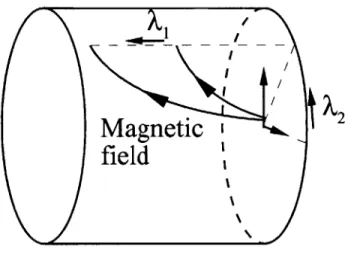
In this problem, two quantities, 0* and T, are almost constant along the lines. Thus, the problem is, basically, 2D. Considering this, the problem can be solved in some other, more natural, coordinates. Let us define A,, A2 and s such as:
b-VA, =0 (2.37)
- VA2= 0 (2.38)
Ox
=b9 (2.39)
as
where x = (x, y, z) are the spatial coordinates.
Note that each magnetic field line is defined by the two values A, and A2 (thus,
these variables are constant along magnetic field lines). s is the distance along each of these lines.
We require Vs - (VA, x VA2) > 0. We can also impose VA, -VA2 = 0, but this
last condition is very restrictive and can be relaxed.
As an example, consider a magnetic field with cylindrical symmetry and no az-imuthal component. In this case, the variables A, and A2 could be the magnetic flux
function and the azimuthal angle (see figure 2-2).
Using this new reference system, the equations can be cast into a form that deals with the anisotropy in particle and energy transport. Each magnetic line has a unique value of 0* and T. Thus, these variables are functions only of A1 and A2. The other
spatial variable, s, is not necessary to determine the spatial distribution of
#*
andTe. In order to simplify the problem, the equations are integrated along the magnetic field lines. 'Integration along the magnetic lines' is a short name for integration in the volume of a streamtube around the magnetic line (in the limit of a streamtube with infinitesimal section).
The integration along the magnetic lines of a quantity Q is:
im1 Ltemue 3)=[2
lim ft d3X
Q(x)
= 2 ds J(s, A,, A2) Q(s, A1, A2), (2.40)Magnetic
2field
Figure 2-2: Magnetic coordinates field.
A, and A2 in an axisymmetric, meridional magnetic
where the streamtube of infinitesimal section is defined by [Al, A + AA1] x [A2, A2 +
AA2], and J is the Jacobian of the transformation,
J (x, y, z) Ox Ox Ox
J(s,
A,
) A2 - O- - x .0 (s, A 1, A2) aS (OA, OA2)
(2.41)
The integration along the lines is useful because it eliminates two of the unknowns: the transport along the lines, geb and qeb.
Note that equations (2.14) and (2.25) contain, mainly, the divergence of differ-ent vectors (as they are conservation equations). Inside the divergence terms, the transport terms Jeb and qeb appear. Integrating along the field lines will eliminate such terms. The transport along the magnetic field lines can be recovered from the boundary conditions once 0* and T are known. No much information is lost when integrating over the lines and eliminating the terms that contain Jeb and qeb. Due to the high diffusion along the magnetic field lines, the only mission of these terms is to adjust so that the temperature and the thermalized potential are constant along the lines. Thus, once it is known that these magnitudes are constant along the lines,
eliminating the parallel transport is convenient.
In the rest of this section, first the divergence of a vector will be obtained for the new variables, s, A, and A2. In this new form, the process of integration along the
magnetic field lines will give a convenient form that simplifies the calculations. Once this general result is proved, it will be applied to equations (2.14) and (2.25).
2.3.1
Integration of a divergence along the magnetic lines
In the new variables, the divergence of a vector V is:V -V = Vs - + VA - + VA2
-Os OA1 OA2
Then, the integral of the divergence of V must be:
82 ds O si Os (Ox Ox 0A1 0A2) Vs- +VA, Os OV OAi (2.42) +VA2 -
v]
A2 (2.43) To simplify this expression, first consider the following equivalences (these equiv-alences are proven in appendix A):Ox Os Ox (Ox as (OA1 x 11 ) Vs = Ox Ox OA, 0A2 rx OA2) Ox
\
x OA2 Ox Ox Os 0A2 Ox Ox VA2 =- x Os 0Ai Ox 1 1S0A 2) Vs -(VA1 x VA2) -IVA, x VA21
(2.44)
(2.45)
(2.46)
(2.47)
Using equations (2.44), (2.45), (2.46) and (2.47), we can simplify (2.43):
Sds
JV-V j82 Si S ds-[aBs
(
VAVs-V1 x VA21) O VA -V 0A VA1x VA2! _ VA2 V _)] OA2 I VAI x VA21 (2.48)J
812 dsJV-V= Ox (Ox s 0A, Ox OA,ax
ax
as (aA1
To get to this equation we have used:
A Vs
V x VA +
(
VA, A) +0A1 IVA x VA21
O
(
VA2 0A2 IVA1 x VA21 Ox 4 -x O 11 ) +OA 8x x \0OA,
= 0 (2.49)Equation (2.48) is important because it allows us to simplify the equations. Inte-grating in s, that is, along magnetic field lines:
I d[( Vs -V
+
V -V
SO
as
IVA1 x VA21 OA1 IVA x VA21Vs - V OsB VA, - V
IVA, x VA21 OA, IVA, x VA21
+ 0 fds V, + OA, I VA x V VA2 O A
(
VA
2 V ) 2 IVA, x VA21 asB VA2 -V i 0A2 IVA x VA21 S(1si VA2 - V A2 So IVA x VA21)2.50) Here, SB(A1, A2) is the equation that describes the boundaries of our domain. SBcan be so or si.
Considering that F = s - sB(A1, A2) = 0 is the equation for the boundary:
VF Vs - OsB
VA-OA, OSBVA = 0A2 kN
where
N
is the normal to the boundary, and k is simply the magnitude of the vector. It is also true that:k -
N
= b Vs - asBOA1
0B
OA2 *VA2 = Os .Vs = 1 Then, k = 1/(b -
N)
and we can write:Vs- VA,
OaA
OsB __N
OA
2 b- NFinally, the integral of the divergence of V along the magnetic field lines can be
0s (2.51) (2.52) (2.53) as OA, 0 ( x OA, as
written as:
S2 VN +
N +
sJ (b N)IVA, x VA21 (=-
N)-VA,
x VA21 =+ ds VAV + ds VA2 V (2.54)
j sO IVA x VA2 ) 0A2
(Lo
IVA x VA21where VN = V -N.
N
is defined to be the normal pointing out of the domain. Therefore, -N
has different sign on both endpoints of the magnetic field line.2.3.2
Charge conservation in the new variables
Let us apply the divergence integrated along the magnetic lines to equation (2.14). It is important to notice that this equation contains three different types of terms: Hall terms, where the vector inside the divergence is, for example, V = -b0H X VO*; perpendicular collisional terms, where the vector inside the divergence is, for example, V = -a IVi#5*; and parallel transport terms, where V = bjeb. Let us deal with an example of each of this type of terms.
First, consider that b. V#* = 0 and b -VTe = 0, which means:
ao*
ao*
V#*
= V 5 + V* (2.55)VTe = VA, + VA 2 (2.56)
Now, let us work with the Hall term for
#*.
In the new variables, and after integration along the lines, it is:a
([Sids JHVA1 -(1 x Vq*) 9 ([ dsJHVA
2 X Vq*) (2.57)d4
sO 1VA x VA21 - sO VA1 x VA2I
Considering that b - (VA, x VA2) = IVA x VA21 (see Appendix A):
9(f1 _HV_1 - Xs x *) u 1 ds HVA2 - X Vq*)
9A, &A2) cH =
/
dso~H where _(#*
a U :Ha9A
2OA,)
This expression for the Hall term can be made more compact if we define the operation (vI, v2) x (wI, W2) = v1w2 - v2w1, and the operators VA = (0/0A1, a/OA2)
and Vx\ = (-a/A 2, O/A,). The Hall term becomes:
-VA -(5HVx#b*) = -VA7H VxA# = *x VAH (2.60)
This means that the divergence of the Hall current is zero if
#*
= f(5H). More will be said in the next section about this.Now, working on the perpendicular collisional term for 0*:
a
([S1 0A, IOOA,
-LVl -V ds V VA2#* OA24 OA_ -a (U-L,125)
OA _ A#* 12 '9 A ds -O =-V2- dVA1 x VA21(
,22 2.61) wherei1,=ij ds o VA- VA for i = 1, 2, j = 1, 2 (2.62)
SO IVA x VA2
In a case where VA, -VA2 = 0, the equations are simpler because 3i1,2 = a1,2 1 = 0, I,l = f -IVAI/IVA2Ids and 61,22 = f oLIVA21/IVAIds.
This term can be also made more compact by using the matrix b1
EU
1,2 1 1,22(2.63)
-VA
-
(5-
-VA#*)Finally, let us consider the parallel transport term:
ds jebb
VA,
1VA x VA2I + a( OA2 so ds Jebb VA2 IVA x VA2I0 (2.58) (2.59) ax (1:1 a8 i (2.64)0#*
'"L, II9A)This cancellation is the main advantage of integrating along the lines. Working all terms similarly, equation (2.14) becomes:
Te Te (2.65) where yH = - dsrH I-n ne )(-26 ) \ no V
aI
=( ,Sd , = - ds o 1 - In (2.67) 771, 12 '71,22 S- 1 ds V ,a
ds (2.68)aK
L
0 IVA, x VA2 aA2 so IVA x VA21SW= - YjiN + YeN iN + jeN
(b - N)IVA, x VA2 I (b- N)IVA, x VA21
Si is the divergence of the ion current, taken here as a given quantity. S, is the wall charge loss. It depends on the interaction plasma-wall. Around the walls, non-neutral sheaths form. The behavior of the plasma in those sheaths and their effect on the quasineutral plasma determine the charge and energy flows to the wall. In the case of dielectric ceramic walls, the current to the walls is zero. Then, wall charge loss is S,, = 0. For a conductor wall, the condition is not that simple. However, only
the anode and the cathode are conductors in usual Hall thrusters, and these elements are dealt with independently, not as source terms.
2.3.3
Energy equation in the new variables
Similarly, equation (2.25) becomes:T T
C e - VA -(HVxXO* ~ VA -HVxA
at
e e-VA - (!!- - VAO*) -VA -L - VA =e Et + Ej + Ew (2.70) e
[ 1 3 e ns soo 2 1VA X V A2 d Te [d[s n + EH e JLuH2 oJ 0* 1* s Jd H ds VA VA In -e + jVA x VA21 2 no I +#*JdscujL7)i . VA3 IVA x VA21 (In ' )2] F1 , 11 1,12 1 1) I 9
I
Te + (In n )21I
ds aL VAj VA1x VA21 - 0*J
ds ds [(3 IVA x VA21 2 Is1 ds E=- enevi ,0 IVA1 x VA2 E = QeN (1 N)IVA x VA21 =,oE5
VAj - VA-cVA1 x VA21 7 2 1 in-+ In + no ne no] - #5*1 (ene) Otai
+0*+
e Te In he e no QeN (N)IVA, x VA21 8=QeN is the total energy flux perpendicular to the boundary:
( Te
QeN
= qeN - jeN -*)
5
-) = eN - jeN 2~
Et is the change in energy due to the variation of electron density. Time variation of the electron density implies time variation of the electron thermal capacity, and, therefore, a change in temperature. Ej is the ionization loss. The model used is the same as in [5]. where EI,11 E1,12 (2.71) (2-72) z 1,12 E-, 2 2 dsUH 15
I
- = 7 2 - Te eI
(2.73) (2.74) Et = -so1 (2.75) (2.76) (2.77) (2.78) (2-79) I I - ' I - In ne T no) e - In n e no) e dsUH 1- In n I no]E, is the energy wall loss. It depends on the non-neutral sheath behavior. A
good model is the one proposed by Ahedo et al. [15]. This model takes into account the electron secondary emission from the wall. The secondary emission may be quite large for ceramic walls, and it has an important effect: the Charge Saturation of the non-neutral sheath. The Charge Saturation is reached when a small potential well is formed in front of the wall by accumulation of electrons there. That small well repels most of the secondary emission back to the wall and keeps the electron current coming out from the wall almost equal to the incoming current (see [15] for more details).
Charge Saturation is important because the outgoing electron current is large and almost cancels the current of electrons originated in the plasma, allowing for an incoming electron current much larger than the incoming ion current. That huge electron current carries the energy from the electrons into the wall, giving place to a
rather large energy loss once the Charge Saturation is reached.
Figure 2-3 shows this effect. Note that the Charge Saturation Limit (CSL) is reached for Te ~ 20 eV. Around that temperature, the energy wall losses grow drastically. That tends to keep the temperature under 20-30 eV because the energy losses above these values are much bigger than the energy sources in the system. This is important in the physics of Hall thrusters, because it keeps the electron temperature at low values.
2.3.4
General considerations about the 2D equations
Equations (2.65) and (2.70) are equations for 0* and T. Before, jeb and geb were also unknowns, but integrating along the lines has eliminated these variables. This integration has also eliminated the dependence with s. Only the dependence with Al and A2 is left. These variables determine uniquely each magnetic line. The best way to visualize these variables is considering an axisymmetric magnetic field. Then, any cylindrical surface is cut once and only once by each magnetic line, and each point in the cylindrical surface corresponds uniquely to a magnetic line. That is what is plotted in figure 2-2. Al is equivalent to the axial coordinate in the cylinder, and A2
I I I I I
n.
=10 m CSL I I - I-5 10 15 T (eV) 20 25 30Figure 2-3: Wall energy losses for a typical ceramic wall density is fixed at ne = 1017 m-3.
at different T. The plasma
is equivalent to the azimuthal angle.
It is interesting to take a look into the form of the equations. There are terms derived from the Hall transport, such that
-VA -(HVxAO*) = VAH X VO* (2.80)
These terms are characterized by the lack of second derivative and they are usually the higher order terms in the equation (by a factor we/ve).
The collisional perpendicular transport terms are diffusion-like, such that
-V,\ (57L I ,\* (2.81)
Since these equations have been integrated along the magnetic lines, the flows across the boundaries appear:
jiN + jeN JiN + jeN
(b -N)1V1A x VA2I +, (b -N)IVA, x VA2 j 250 200- 150- 100-C" 501F OL 0 (2.82) I .I I I I
Any other term is just the corresponding contribution from equations (2.14) and (2.25). Finally, let us sketch how to recover Jeb and qeb. Using equation (2.48), but without integration along s, equation (2.14) can be rewritten as:
(( jeb
)
09s IVA x VA21a(
VA1 -jrest
+A
1IVAi
xVA
21
+ (VA2 - rest ) ++- 0 ( s -irest
0s IVA1 x VA2I = 0
irest = JeH + Je-L + i (2.84)
jrest
is known once q* and Te are found. Then, jeb can be calculated along each magnetic field line by integrating in s. Only one boundary condition is needed. The boundary condition can be found from the known value jeN + JiN at one of the endpoints of the magnetic field line:jebls=so =
(JeN + iN) s=so irest s=so N
(2.85)
geb can be found in a similar fashion:
qeb - (2e/J)jeb VA1 x VA21
)
+ VA, -Qrest +A a VA x VA2I)a
Vs
Qrestas
IVA x VA2/
a
(VA 2 - Qrest + aA2 VA1 x VA2Ia
+ -t
3 - ene -Te = Ei, whereQrest
is known once q* and Te are known.2.4
Structure of the 2D solution
Both equations (2.65) and (2.70) have similar structure. To study the possible solu-tions, let us take equation (2.65) for the simplified case Te = const. and VA1 -VA2 = 0: -VA -(_6:VxAq5*) - VA -
(&-
-VXO*~) = S (2.87) where(2.83)
a
as
(
where UH, &_ = ± '11 and S are known functions of \1 and A2.
[0
5:1,22]Note that what was pointed out for the 3D equations is still valid. The Hall transport term can be rewritten in a more convenient way:
-HVxAO = -= xAH + xH*V (2-88)
This means that the Hall current can be divided into two parts: a divergence-free current and a term that looks like convective transport for
#*.
This term has a 'drift velocity', VdA = VxA5H. Now, plugging this back into the equation:VA - (O*VxA&H) - VA -(6;- .VA\*) = S (2.89)
Looking at the order of magnitude of the different coefficients, the term that contains YH is much larger than any other term by a factor we/le. This means that, to zeroth order:
VA - (O*V x:H) -- VAH X VA# = + -- ~ 0 (2.90) 0&\1 0A2 +&A2 &A1
This equation imposes that
#*
is constant along the lines H = constant. The convection-like transport makes the thermalized potential, 0*, uniform along the 'drift lines'. The 'drift lines' are the lines parallel to VdA. These are lines in the A, - A2plane, which are magnetic flux surfaces in the 3D problem.
Note that equation (2.90) may not (and usually will not) be enough to determine
#
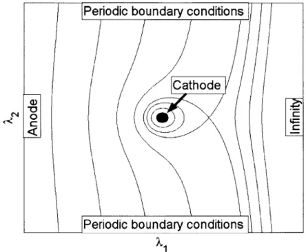
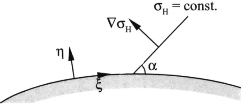
since its variation across 'drift lines' is left indeterminate by the neglect of the higher order terms. Let us look at a usual Hall thruster configuration plotted in aA1-A2 plane (see figure 2-4). Assume that A, and A2 are the axial and azimuthal
coordinates that locate the magnetic field lines (as seen in figure 2-2). A typical configuration of DH = const. lines is plotted in the A plane. The definition of UH is
given by (2.59) and (2.9). Considering that ve< we:
/en
Jen
- IBe ds (2.91)
Note that TH is almost azimuthally symmetric far from the cathode. The effect of the cathode is a peak in UH, due to the increase in electron density in its vicinity. There is a saddle point after the cathode and away from the anode. This is due to the competition between the growth of UH as we get away from the thruster and
the decrease of the same quantity as we get away from the cathode. UH increases away from the thruster because the magnetic field strength decreases. Hall thrusters have a dipole-like magnetic field that decay as r-3, where r is the distance from the thruster. The density, modelling the expansion of the plasma as if the pressure followed a simple politropic law, p oc ny, decays as r- 4/(l+,). That means that for
r -* oc: 4
/ene
r I+, 4-_H Br- d oc r3 r = r 4+y (2.92)
Since 7y> 1, UH grows as we go away from the thruster; therefore, there is a saddle
point produced by the two counter tendencies: the decrease of 5H when moving away from the hollow cathode and the increase due to the drop in magnetic field strength when far enough from the thruster.
The boundary conditions are imposed on the boundaries A, = const. and on the contour of the image of the hollow cathode in the A, - A2 plane. That means that
only some of the lines UH = const. have information for
#*.
The thermalized potential in the other lines has to be determined by the next order equation, which contains diffusion terms. Chapter 3 is devoted to solving this problem numerically.The question about the validity of this approximation naturally arises. We have to pay special attention to the boundaries and the points where the gradient of UH
Periodic boundary conditions
Cathode
Periodic boundary conditions
Figure 2-4: Hall thruster representation in a A1 - A2 plane. iH = const. lines are
plotted.
Solution at the boundaries
At a boundary, a thin layer will develop. The physical meaning of such a layer will be discussed later. Now, the mathematical solution in such a layer will be studied.
In the 2D space A1 - A2 it is possible to define, at least locally, two variables, and
q (see figure 2-5), such that the boundary that we are studying is a line rj = const.
and is a variable independent of q that follows the boundary.
In such variables, and considering that the gradients along q are much larger than along , the equation for q* would be:
H a _o - 92,7$ =
0
(2.93)
(sin a -±2osa., - _
=
where
/
+ ,22 (2.94)GH
COnst.
vG HFigure 2-5: Coordinate system tangent to the boundaries. Note that the direction of cYH = const. lines is given by angle a.
oH sin a =H + (2.95)
8Ai &A2. aA2 9Ai
HH
cos a = + (2.96)
aAj oA 2 0A2 &
51,7i7, 6c &H and a can be considered functions of only. These parameters do not
change appreciably in 71-direction compared to what they change in i-direction. Considering that , H Ve/e < 1, there are two possible cases:
Sa > ve/We. In this case, the 5H = const. lines are far from being parallel to
the boundary. That means that the equation for the solution near the boundary can be written as:
+ 6oH sin a = 0 (2.97)
Since F,,,,, 6dH and a are only functions of 6, the general solution to this equation is:
= A(6) + B(6) exp 6_ Sin , (2.98)
which shows a boundary layer of thickness 0±,,,/( 65H sin a) (if this is positive).
be an exponential growth. This means, basically, according to equation (2.95):
____H O9 8H 0
a0 19TI +H > 0 (2.99)
&Aj 0A2 OA2 01
where q(A,, A2) = 0 is the boundary we are interested in, and the vector
(&97/9Aj, &97/&A2) points inwards in the plane A, - A2.
If condition (2.99) is not satisfied, there is continuity between the boundary
condition and the solution because there is no boundary layer solution, that is, the boundary layer solution has exponential growth. This means that the value of q* in each iH = const. line is given by the boundary conditions on the boundaries that DO NOT SATISFY condition (2.99). The boundary con-ditions on the boundaries where (2.99) is true do not necessarily determine the thermalized potential in the H = const. lines.
* a ~ Ve/We. In this case, the UfH = const. lines are almost parallel to the boundary. Then, the equation for * is:
0'1 + 5-H sin a
+
cosa =0 (2.100)This is a parabolic equation, where not only the y dependence is important. No general conclusions can be drawn from this equation. However, the boundaries are not expected in general to be parallel to the cYH lines, except in small zones.
The mathematical solution of the problem makes necessary the presence of these boundary layers. The thickness of these layers is 6 = LVe/We in general, and 6 = L /ve/We when the boundary and the UH = const. lines are parallel. L is the
charac-teristic length in the problem, associated to the density and magnetic field gradients. The thickness of the layers can be written in terms of the collision mean free path,
Amfp, and the Larmor radius, PL. In such variables, 6 = PLL/Amfp. If Amfp is assumed to be the mean free path of classical electron-neutral collisions, the thickness 3 would be a small fraction of the Larmor radius, which makes no physical sense since the