IdEP Economic Papers
2019 / 01
G. Masiero, M. Santarossa
Earthquakes, grants and public expenditure:
how municipalities respond to natural disasters
Earthquakes, grants and public expenditure: how
municipalities respond to natural disasters
∗Giuliano Masiero1,2 and Michael Santarossa3
February 2019 Draft version
1Department of Management, Information and Production Engineering, University of Bergamo, Italy 2
Institute of Economics (IdEP), Universit`a della Svizzera italiana (USI), Switzerland
3Department of Economics and Management, University of Pavia, Italy
Abstract
We analyze the response of municipalities to the occurrence of natural disasters (earth-quakes) in Italy, in terms of spending behavior, use of upper tier transfers and recovery. We find evidence of increasing expenditure for about 12 years after the shock, with asym-metric responses between matching (earthquake-related) and unconditional grants, and heterogeneous flypaper effects across the country. While in Northern municipalities ex-penditure tends to regress to pre-treatment levels, i.e., before the earthquake occurrence, Southern municipalities react to the drop of grants showing inertia in expenditure lev-els. This evidence is coupled with a faster recovery of private income and housing prices in Northern municipalities. Our analysis exploits balance sheet data of about 8000 mu-nicipalities for the period 2000-2015 and encompasses the universe of earthquake events defined using alternative intensity measures. We apply a matching approach to disentan-gle earthquake-related grants (mostly matching grants) from other grants, and to define a control group of non-treated municipalities. The spatial and temporal variation in ex-penditure and transfers between treated and not-treated governments are then examined using panel data models on the universe of municipalities as well as on a matching sample of municipalities.
Keywords: Natural disasters, Local expenditure, Intergovernmental transfers, Matching grants, Flypaper effect, Economic growth
JEL codes: H52, H72, R7
∗
Corresponding author: Giuliano Masiero, Department of Management, Information and Production Engineering, University of Bergamo, via Pasubio 7b, 24044 Dalmine (BG), Italy (giuliano.masiero@unibg.it). We are grateful to Massimo Filippini and Fabrizio Mazzonna for con-structive suggestions and useful advice for further improvement of the preliminary analysis. Also, we thank Rosella Levaggi and other participants to the DREAMT Workshop 2019 in Pavia, and to the XXX SIEP Conference in Padova for numerous helpful comments.
1
Introduction
Natural disasters have several implications on affected economies and society. In-frastructures get damaged and need to be repaired, people get injured or die, economic activities are unable to operate and inequalities may worsen (Bui et al., 2014; Kahn, 2005; Str¨omberg, 2007). Whether it is because of legal rules, solidarity or to raise the consensus of the electorate, public authorities commonly intervene by means of higher spending levels and transfers of financial resources from the central government to disaster areas (Barone and Mocetti, 2014; Noy and Nualsri, 2011).1 It has been noted that expenditure on post-disaster relief is generally less efficient and effective than expenditure on prevention (Healy and Malhotra, 2009; Skoufias, 2003). However, governments prefer to deal with disaster relief measures since the electorate is more likely to perceive (or misperceive) the benefits and, therefore, to provide political consensus (Zaman et al., 2010). Despite the involve-ment of local authorities and their role as the main channel of interaction between citizens and regional/central governments to face natural disasters, there is lacking evidence on the response of local public expenditure in terms of resources use and timing, and the subsequent impact on recovery (Bevan and Cook, 2015).
This paper investigates the response of local government expenditure to natural dis-asters exploiting detailed data on expenditure and transfers from the universe of Italian municipalities for a 16-year period (2000-2015), and a large historic data set of seismic events since 1000 AD. To this aim, we estimate expenditure variation following earthquake occurrence using panel data regression models on the universe of municipalities as well as on a matching sample, focusing on immediate and medium-run effects of earthquakes. Further, we exploit the variability in transfers received for earthquake damage recovery to identify a possible source of inefficiency in post-disaster interventions, i.e., the overre-action to transfers from upper tiers to lower government levels that can offset the growth of income - the so called flypaper effect (see e.g., Gennari and Messina, 2014; Hamilton, 1983). Due to their essential matching-grants nature and their duration, the response to earthquake-specific transfers may be more pronounced as compared to other sources of transfers, implying both an income and a substitution effect (Bailey and Connolly, 1998) and leading to persistent path-dependency of local governments expenditure over time.
1
In Italy - a country frequently struck by earthquakes - the central government allocated almost 100 billion Euro at 2014 prices to fund disaster relief just for the five largest seismic events that occurred between 1968 and 2002 (Di Giacomo, 2014).
We apply a matching procedure to disentangle different types of grants and explore dif-ferences in the response to earthquake-specific and general grants. Then, we investigate the asymmetric responses to increasing and decreasing grants and between Northern and Southern municipalities in terms of resources allocation and recovery.
We find that an earthquake increases local government expenditure immediately after the shock by about 2%, following an inverse U-shaped trend, which persists for about 11-12 years since the disaster. This increase is mainly driven by transfers of financial resources from the central and regional governments. Further, we find evidence of flypaper effects with asymmetric responses to matching (earthquake-related) and unmatching grants and to increasing and decreasing grants. Finally, we testify differences in the response of Northern and Southern municipalities, suggesting that the less efficient use of earthquake-specific grants by Southern municipalities lead to poor economic outcomes.
Despite the size of public resources employed in the recovery from losses of natural disasters and the long-lasting effort of public authorities, only a few studies analyze the response of public expenditure to natural disasters and its impact. Melecky and Raddatz (2011) investigate the effect of natural disasters on fiscal sustainability using data on a number of high and middle-income countries for the period 1975-2008, and show that public expenditure grows to allow for recovery. Noy and Nualsri (2011) find that govern-ments of developed countries tend to support more disaster areas by means of transfers of financial resources, while governments in developing countries are less committed or even contract the resources transferred to disaster areas. Other studies focus on the impact of natural disasters on economic growth and show that economic gains are context related (e.g. Barone and Mocetti, 2014; Cavallo et al., 2013; Skidmore and Toya, 2002). Looking at two Italian regions struck by severe earthquakes in 1976 and 1980, Barone and Mocetti (2014) show that in the medium-run (i.e., the first 5 years after the disaster) transfers from the central government allow to entirely cover the losses, but remarkable differences are observed between the two regions in terms of ability to recover. Hornbeck and Keniston (2017) find that Boston city reconstruction after the 1872 fire is an example of successful recovery with beneficial effects on land and house values and urban growth, while Horwich (2000) finds that the port of Kobe in Japan, struck by a severe earthquake in 1995, was able to recover from damages within one year, but economic growth slowed down because part of economic activities moved to other port cities.2
2Note that Horwich (2000) uses information on 19 months after the disaster. This does not exclude that
Our analysis contributes to a deeper knowledge of the effects of post-disaster public spending, which helps policy makers to design more effective and efficient relief measures. Usually, natural disasters affect a limited area of a country and, even if an event is not catastrophic, damages may be remarkable at local level. Hence, observing the conse-quences of these events from a within-country perspective may improve the precision of the analysis. The large majority of studies mentioned above focus at country level and analyze the economic impact of the largest natural disasters, neglecting smaller but harm-ful disasters. Clearly, cross-country studies can only exploit a limited number of rare and big events, which may undermine the validity of the results. Our approach allows to cap-ture the effects of relatively small events since we exploit data for the universe of Italian municipalities and a unique historic data set of all seismic events. Italy is an ideal setting because the country was struck by several hundreds of earthquakes over the last decades, out of which only 19 were large catastrophic events.3 Moreover, local governments are responsible for housing services, urban road maintenance, economic development, social protection and education, all aspects that are likely affected by catastrophes.
The rest of the paper is structured as follows. Section 2 describes the institutional setting and how public authorities respond to natural disasters. Section 3 presents the data and some descriptive evidence on the incidence of earthquakes and changes in public expenditure. Section 4 defines the empirical strategy and Section 5 presents the main results on expenditure behavior and provide some robustness checks. In Section 4.2, we extend the analysis to investigate the role of transfers, and in Section 5.3 we explore differences in the response to earthquakes, i.e. asymmetric responses to increasing and decreasing grants and heterogeneous flypaper effects across municipalities. Finally, in Section 5.4, we further explore differences in the response of Northern and Southern local governments in terms of timing and spending composition, and the effects on economic growth. Section 6 concludes.
(2002) after city bombings in Japan during World War II.
3
Our elaboration on data provided by the Center for Research on the Epidemiology of Disasters (CRED) (Guha-Sapir et al., 2017).
2
Institutional and seismic background in Italy
2.1 Exposure to earthquake risk
Italy is a country with a high frequency of earthquakes. The country is almost contin-uously exposed to minor earthquakes and several large events occurred both recently and in the past. However, it is necessary to distinguish the physical strength of an earthquake from the damages it causes. A very strong earthquake that occurs in a not populated area without infrastructures may not cause any damage, while a mild earthquake that strikes a town with weak infrastructures may cause human losses and large damages. The 2017 earthquake of Ischia was a relatively weak earthquake (moment magnitude 4), but very destructive because of poor building standards present in the area. This distinction is of relevance also because Italy is rich in cultural heritage, which is difficult to protect against natural disasters.
Figure 1 illustrates the frequency of earthquakes with intensity equal or bigger than 5 at municipality level for the period 1985-2015. Intensity 5 is the lowest level at which damages occur (see Section 3.2 on earthquake measurement for details). The map highlights that earthquakes occur across the entire country. One-third of municipalities were struck at least once by a seismic event over the considered period and almost half of them in the period 2000-2015. The areas most frequently affected are the regions Emilia-Romagna in the North, Umbria, Marche, and the municipality Rome in the Center, Abruzzo, Basilicata, Northern Puglia and Eastern Sicily in the South.
The exposure to earthquake risk leads to the classification of municipalities into seismic zones. In 2004, the Italian Institute for Geophysics and Volcanology (INGV), a unit of the Civil Protection with the task to increase the knowledge on the Earth system and its phenomena and to monitor seismic and volcanic events, analyzed the probability to face large earthquakes based on the movement speed of the ground and defined, accordingly, 4 seismic zones. A more detailed classification with sub-categories was realized in 2015. This classification is of interest for the central government because it allows to address policies to the most exposed areas. One of these policies defines building standards that must be fulfilled in high-risk seismic zones. Moreover, the central government allocates funds for infrastructure maintenance to prevent disaster damages based on the classification.
2.2 Administrative organization and response to natural disasters Italy is a decentralized country where the public administration consists of 4 levels: the central government, the region, the province, and the municipality. The main task of regions is the provision of services in the health care sector. Provinces are responsible for the maintenance of non-urban roads, environmental protection and secondary education. Municipal governments are required to offer a number of services, among which the most relevant are local transports, urban road maintenance, waste disposal, housing, social protection, and primary education.
Since the early ’90s, the administrative organization has changed. The Law 142/1990 started a decentralization process of powers from the central government towards local authorities with the attempt to increase the autonomy of local governments. This implied a change in the composition of funding sources. Since 1992, an increasing share of local government revenues derived from the withholding of tax revenues, mainly from property taxes and surcharges on income taxes, and from the revenues generated by local service provision. However, decisions on local tax rates are constrained by national regulation that limits the extent to which local governments can leverage on taxation. The central government reallocate resources among local governments with the purpose to grant equal access to essential services across the country. In 2002, a fund for equalization was es-tablished. The resources are distributed to local governments, both directly and through regional governments, so that governments with insufficient own resources are able to pro-vide the necessary services to the population.4 To grant equal access to basic services across the country, the central government funds up to 70% of the expenditure reported in the balance sheet of the year before.5 The other services need to be funded with own resources.
In 2015, local governments spent 83 billion Euro, which is 10% of total public expen-diture in Italy. Transfers of financial resources from the central and regional governments and from other public institutions account for 14% of current revenues. These transfers are mainly unconditional. Current transfers represent on average 70% of total transfers and
4
The benchmark adopted by the central government is the average revenue of municipalities of a given demographic class. Decree Law 267/2000 (Testo unico delle leggi sull’ordinamento degli enti locali ) classified municipalities into 12 demographic classes based on the size of the resident population and defined regulation accordingly, because population size determines differences in needs.
5
Since 2009, services provided by local governments are divided into basic services and other services. Basic services are general administration, local police, education, local transport, social protection and local services. Local services are housing, Civil Protection, waste disposal, water services, and services for environmental protection.
they are generally non-earmarked transfers, while the remaining share represents capital transfers, which are generally distributed for specific projects, such as the construction of infrastructures. The remaining 86% of local government revenues is composed of own resources. Almost half of own resources are produced by local taxation (ISTAT, 2017).
The response of public authorities to natural disasters consists of two phases. Imme-diate aid is provided to meet short-run needs, such as the provision of food and medicals, the preparation of emergency camps, and the inspection and evaluation of damages to infrastructures. Later on, effort is put in the recovery from losses and in the prevention of future disasters. Generally, funds for recovery from damages are matching grants, i.e., they meet spending requirements for specific projects proposed by local public authorities. Although central authorities are not obliged to intervene in the case of natural dis-asters, usually they offer immediate support through the Civil Protection Department.6 Moreover, the law empowers the central government to claim the state of emergency and define its duration and the involved area (Art. 5 of Law 225/1992). This claim has two main implications. First, the central government can recur to decrees to face the situa-tion notwithstanding the current regulasitua-tion. In this way, public authorities can intervene immediately without the need to recur to legislative procedures, which could impede a prompt and proper response to the catastrophe. The second implication is that the state of emergency allows to transfer financial resources from the fund of the Civil Protection to the affected areas. However, this procedure can have a drawback in terms of timing. The central government can claim the state of emergency only upon request from regional gov-ernments through the Civil Protection. Commonly, regional govgov-ernments decide whether to ask for the state of emergency based on the size of damages. They delegate the collec-tion of informacollec-tion from the citizens to local governments, a procedure that could delay effective intervention.7
For medium and long-run support to disaster areas, the central government needs to follow ordinary legislative procedures. Based on the size of damages resulting from inspec-tions, financial resources for the reconstruction of capital and the recovery of economic
6The Civil Protection Department, which is administered by the Presidency of the Council of Ministers,
guides the prevention, response, forecast and risk monitoring activities related to both natural and man-made disasters through central and local units across the country.
7
In 2002 and 2003, further regulation was introduced in order to reduce the time of response and the exposure to seismic risk. In case of extreme events that threaten lives of individuals, the government can assign special powers to a delegate even before claiming the state of emergency (Art. 3 of Law 245/2002). Also, an additional fund, managed directly by the premiership, was established to transfer resources to regional and local governments for both prevention and disaster relief (Art. 32-bis of Decree Law 269/2003).
activities are allocated by means of decree laws. A final tool at government disposal is the yearly financial law, which allows to allocate additional resources to the areas affected by catastrophic events.
3
Data and descriptive evidence
3.1 Data
In this study we use 3 main data sets: (1) local government balance sheet data, (2) data on earthquake occurrence, and (3) data on municipality characteristics. Data on local government expenditure are available for 7997 Italian municipalities observed for 16 years (2000-2015).8 The panel data set is obtained from the Italian Ministry of the Interior and contains detailed information on expenditure as well as revenues of local governments for each year.9 Our measure of expenditure (revenues) is the sum of current and capital expenditures (revenues) registered in the competence and residual accounts in each year.10,11
We gathered data on earthquakes from two databases available from INGV that collects information on earthquake occurrence between 1000 and 2014.12 The first database is the parametric catalog of earthquakes CPTI15 (Rovida et al., 2016) that includes detailed information on each earthquake (e.g., magnitude, maximum intensity, coordinates of the epicenter). The second database is the macro-seismic database DBMI15 (Locati et al., 2016), which reports local earthquake intensity measures. The selection criteria for the inclusion of an earthquake in the databases are either a maximum intensity equal to or greater than 5 on the Mercalli scale, or a moment magnitude equal to or greater than 4.13 Although data on earthquakes for 2015 are not available, their impact is likely negligible
8
A small number of municipalities merged over this period. Therefore, to construct a homogeneous panel over the entire period, we aggregate the data of merged municipalities in the years before the merger. We replicate the 2016 municipality structure because some data are available only for that level of aggregation.
9Actually, we have data for the period 1990-2015 but differences in the statistics before 1998 and the
lack of data on household income in 1998 and 1999 advise not to use those data before 2000.
10The competence account registers expenditures and revenues related to cash flows, while the residual
account registers transactions for which the cash flow has not occurred yet.
11For the years 2000 and 2001 currency values expressed in Italian Lira were converted to Euro using
the fixed exchange rate of 1,936.27.
12
https:// emidius.mi.ingv.it/ CPTI15-DBMI15/ .
13
The intensity is measured on the Mercalli scale and quantifies the observed effects of an earthquake on a scale from 1 to 12. The moment magnitude is a logarithmic scale that measures the energy released by an earthquake. A unit increase in the scale corresponds to 101.5 times higher released energy. While
the magnitude is measurable with instruments, the intensity is an evaluation performed by experts based on the observable effects on humans, infrastructures and objects.
since INGV stated that fewer earthquakes occurred than in 2014 and only 18 shocks had a magnitude equal to or above 4, no one bigger than 5.
The third data set includes socioeconomic, sociodemographic, and environmental char-acteristics of Italian municipalities between 2000 and 2015. In particular, the data set contains data on income levels, sourced from the Department of Finance of the Ministry of Economics and Finance, data on population size, age structure and environmental char-acteristics sourced from the Italian Institute for Statistics (ISTAT), and political charac-teristics sourced from the Italian Ministry of Interior. Moreover, we use data on minimum and maximum housing prices (per square meter) provided by the Real Estate Market Ob-servatory of the Italian Revenue Agency. These data are collected twice a year and are complete since the second semester of 2003.
The total number of observations (municipality×year) is 127,952. Balance sheet data and political variables are not complete for 8,076 observations. Therefore, our final data set is an unbalanced panel composed of 119,876 observations.
3.2 Measurement of earthquake occurrence
Two measures of earthquake occurrence can be used to identify municipalities affected by earthquakes (treated municipalities): the magnitude and the intensity. The magnitude is an objective measure of the strength of an earthquake and its ability to serve as a proxy for damages to human and physical capital may be questioned. Since the magnitude is a space-invariant measure, some assumptions on the propagation of the effect in terms of distance and direction are required to assign earthquake events to municipalities. Gen-erally, the propagation of earthquake waves depends on the depth of the epicenter and on the characteristics of the soil. Instead, intensity is the result of the evaluation of the observable impact performed by experts, who usually inspect disaster areas immediately after the shock. One cannot exclude that this evaluation is to some extent affected by sub-jective judgment driven by emotional involvement (e.g., attachment to the disaster area or to people who live there) or even corruption (e.g., the overestimation of the impact of an earthquake could allow to attract more financial resources from upper-level govern-ment). However, intensity is assessed for each municipality affected by an earthquake and allows easily to identify towns affected by damages due to the shock. In our analysis, we prefer the intensity-based measure of earthquake occurrence because this is a qualitative measure of the local impact of an earthquake and varies among municipalities. The use
of fixed effects in our econometric models should address any claim of systematic bias in the measurement of earthquake occurrence due to subjective judgment correlated with the geographical/institutional setting. More than that, we perform robustness checks of our results based on the described magnitude-based measure of earthquake occurrence under different assumptions of propagation. We provide a more detailed description of this approach later on in Section 5.1.1.
We assign treatment if a municipality is struck by at least one earthquake with intensity >5 in a given year. We choose this threshold because 5 is the lowest intensity level at which damages usually occur, and because it is the minimum intensity level for which we have complete data. Then, we define a set of treatment dummies EQi,t−j = 1, where i denotes the municipality and t the year, if the local maximum intensity of earthquakes occurred in the year t − j (with j >0) is >5. This set of variables allows to capture the impact of an earthquake at different points in time before the current year t. Our treatment variables show that 2658 municipalities are struck by an earthquake at least once over the period 1985-2015, and 1129 out of these municipalities are affected at least once over the period 2000-2015.
3.3 Descriptive evidence
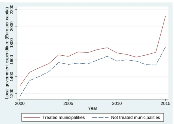
As preliminary suggestive evidence we compare the per capita local government expen-diture of municipalities struck by at least one earthquake over the period 1985-2015 with the expenditure of municipalities that did not face any earthquake during the same pe-riod. Figure 2 shows that, on average, municipalities affected by earthquakes spend more than other municipalities, with a mean difference for the period 2000-2015 of 106 Euro per individual at 2010 prices. In 2015, local governments increased expenditure by 10% on average because the central government loosed the constraints on capital expenditures, which were limited as a consequence of the economic crises in order to attempt to reduce public debt. Clearly, we cannot exclude that this difference is due to factors other than earthquake occurrence, such as institutional differences or historical spending behavior. Indeed, local government expenditure varies both across and within Italian regions, which may be due to factors such as geographical and institutional characteristics and economic development (see Figure A.1 in the Appendix).
To identify the impact of earthquakes on local government expenditure, it would be de-sirable to observe the same municipality under the two scenarios of treatment (earthquake
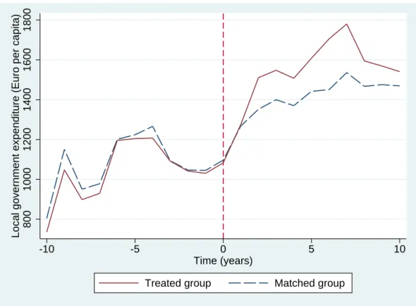
occurrence) and no treatment. Clearly, this is not possible but may not represent a prob-lem if earthquakes are randomly assigned to municipalities. The assumption of random assignment is challenged by earthquake occurrence over time since some areas are more exposed than others. However, a matching procedure that enhances the comparability of municipalities may grant sufficient strength to the analysis. Therefore, we sharpen the evidence of Figure 2 and reduce the unobserved variability, by comparing municipalities that are similar in the period before the occurrence of an earthquake. To do this we construct a counterfactual group of municipalities that allow us to analyze post-treatment variations of spending levels and to claim a causal relationship with earthquakes. Figure 3 illustrates the average spending trend of 517 treated municipalities, before and after the occurrence of a shock, with 517 matched municipalities. We identify matched mu-nicipalities with coarsened exact matching on average financial, sociodemographic and socioeconomic pre-treatment characteristics (see the Appendix Section A.1 for further in-formation on the matching procedure and Table A.1 for the balancing properties). Note that, before treatment occurs, average per capita local government expenditure is almost identical in the two groups. Starting from the first year after the treatment period (period 0), expenditure sharply diverges. Treated municipalities seem to spend much more than the counterfactual group. Spending trends start to converge again from the 7th year after the disaster, though not completely.
Table 1 provides some descriptive statistics on the characteristics of 1129 municipalities struck by an earthquake over the period 2000-2015 and 5339 unaffected municipalities. We observe that in the year before the occurrence of an earthquake, municipalities do not significantly differ in terms of per capita expenditure and revenues, while the revenue composition tends to differ in treated municipalities. Treated municipalities collect less local taxes than the control group, which could be due to the lower household income and the higher share of low-income population.14 The lower amount of local tax revenues is partially offset by increased transfers of financial resources from the central and regional governments. The aggregate revenues from local taxation and transfers account for about 60% of total revenues.
After an earthquake, both local government expenditure and revenues significantly
14We define the share of low-income population as the share of individuals earning a yearly income less
than or equal to 10,000 Euro. Note that our income data is structured in 8 income classes and for each class we have information on the total amount of income and the number of individuals. According to our definition, the low-income individuals are those of the two lowest income classes representing about 39% of the total number of individuals.
increase by 198 and 185 Euro per capita, respectively. The immediate increase of revenues allows to limit losses. Additional revenues are composed for more than 60% of transfers from the central and regional governments. Revenues from local taxation, instead, do not vary significantly on average. As for the population size and age structure, treated municipalities are almost twice as populated as other municipalities and, before the shock, they have a slightly higher fraction of the youngest and oldest age cohorts. Population size does not significantly vary after the shock, but the age structure changes since the percentage of young people tend to shrink, while the elderly share increases. This could suggest that elderly people are less mobile because of physical limitations, or stronger emotional attachment to their town.
This preliminary evidence suggests that the comparison of expenditure levels between municipalities affected and not affected by earthquakes should carefully address differences in terms of characteristics that could confound expenditure variations. The following em-pirical strategy controls for those observable characteristics as well as other unobservable time-invariant characteristics.
4
Empirical strategy
4.1 Earthquakes and spending levels
To assess the impact of earthquakes on local government expenditure, we regress per capita expenditure against earthquake measures and control for characteristics of munici-palities and local institutions that may affect spending levels as well as for time-invariant heterogeneity.15 We specify the following model:
yit = Tit0α + x 0
itβ + θt+ γi+ εit (1)
where yit is the natural logarithm of per capita expenditure of municipality i in year t. Tit0 is a vector of treatment variables, i.e., earthquake indicators, and x0it is a vector of time-varying controls, including the intercept term. Controls (x0it) include income, population age structure, geographic and political characteristics, and funding sources from the central and regional governments. α and β are the vectors of parameters to be estimated. θt are time fixed effects, γi is a municipality-specific time-invariant element,
15
The literature has suggested several features of local governments that are likely to affect the expen-diture. See for instance Gennari and Messina (2014) and Lundqvist (2015).
and εit is the idiosyncratic error term.
In our baseline specification Tit0α is defined as:
Tit0α = 1 X j=0
αjEQi,t−j+ EQi,t−d× (αd1Distit+ αd2Dist2it+ αd3Dist3it) (2)
where EQi,t−j and EQi,t−d are the dummy treatment variables described in Section 3.2. More precisely, the two terms in the summation, EQit and EQi,t−1, capture the effect of an earthquake occurred in the current year and one year before, respectively. The shocks occurred earlier (more than one year before) are captured by EQi,t−d, where d is the temporal distance from the most recent earthquake before t − 1 (1 < d 6 15). We define Distit = d if EQi,t−d is equal to 1, and 0 otherwise. Therefore, the distance polynomial of third degree (within brackets) is a non-linear time-trend capturing medium-run marginal effects of earthquakes on expenditure. We consider a non-linear time-trend to capture a possible inverse U -shaped effect and a tail of earthquakes on expenditure.16 Indeed, our descriptive statistics suggest that expenditure initially grows and then tends to converge to pre-treatment levels. We impose Distit 6 15 since beyond this period we generally observe a convergence of expenditure to pre-treatment levels, as suggested by the descriptive statistics in Section 3.3.17
The covariates that compose the vector x0itare a set of time-varying financial, political, socioeconomic, and sociodemographic variables, and a set of time-invariant environmental characteristics. Financial variables include the natural logarithm of per capita transfers from the central and regional governments, and the natural logarithm of per capita rev-enues from local taxation. Political variables include the vote-share concentration of the local government Council, the number of years before municipal elections, a dummy vari-able equal to one if the incumbent government is center-right oriented, and a dummy variable equal to one if the incumbent mayor reached his term limit. Socioeconomic vari-ables include the natural logarithm of average yearly per capita income and the share of low-income population, and sociodemographic variables include the share of the youngest (0-14 years) and oldest (>65 years) age cohorts. Environmental characteristics are
cap-16
We use a third-order polynomial time-trend because, according to preliminary findings, it is the most suitable specification to capture the effect of an earthquake on local government expenditure. Indeed, in what follows we use also a model specification including yearly lags of earthquake occurrence measures (see Section 5.2).
17Preliminary findings suggest that spending levels tend to converge to pre-disaster levels between the
10thand the 15thyear after an earthquake. Moreover, the impact of an earthquake is fully observed for a maximum of 15 periods in our panel.
tured by dummy variables equal to 1 indicating whether a municipality is a partially mountainous jurisdiction, a mountainous jurisdiction, or a coastal jurisdiction.
To estimate the parameters of our model we use three methods: pooled OLS, ran-dom effects, and fixed effects regressions. Pooled OLS provides consistent parameters but treats observations as mutually independent and does not account for serial dependence of observations. Hence, the main limitation of the pooled OLS model is that possible unobserved heterogeneity among municipalities is neglected (γi= 0). However, both OLS and random effects regressions include a region-specific time-invariant effect.18 The ran-dom effects model treats unobserved heterogeneity of municipalities as a ranran-dom shock and requires the assumption that γi is iid. The fixed effects model relaxes this assumption by allowing γi to be correlated with the other exogenous variables, but it does not allow to include environmental time-invariant characteristics and region fixed effects.19 The random effects model is more efficient, but if the assumption on the independence of the time-invariant error is violated, the estimates are biased. In that case, the fixed effects model should be preferred because it estimates consistent parameters. Since several unob-served factors could lead to differences in spending levels (e.g., geographic characteristic, touristic attractiveness, economic development), we expect the fixed effects model to be more appropriate. We formally test this assumption using the Hausman test.
In addition, we specify a first-order autoregressive model and include the lag of the dependent variable as a regressor in Equation 1. This specification allows to capture the persistence of local government expenditure that may be driven by historic and in-stitutional factors. We estimate this model with municipality fixed effects. Since serial correlation and heteroskedasticity may affect the estimation of the standard errors, we use robust standard errors clustered by municipality in all specifications.
An issue that needs to be discussed is the possible endogeneity of upper-level gov-ernment transfers. In Equation 1, we assume that transfers are exogenous, and hence transfers lead to a variation of local government expenditure because more resources are available, as literature in this field suggests (e.g. Gennari and Messina, 2014; Revelli, 2006). However, variations of transfers from upper-level governments may not be completely
ex-18
Note that region-specific time-invariant effects account for heterogeneity between ordinary and au-tonomous regions with special statute (i.e. the regions Valle D’Aosta, Friuli Venezia Giulia, Sicily and Sardinia, and the provinces of Bolzano and Trento), such as differences in the funding mechanism of public expenditure. Moreover, conditional on region-specific time-invariant effects, our regression results are not sensitive to the inclusion/exclusion of autonomous regions with special statute.
19
Two municipalities of the region Marche became part of Emilia-Romagna in 2010. However, this change is not significant.
ogenous to expenditure variations if they are influenced by higher spending requirements (Lundqvist, 2015) or by the ability of politicians to attract financial resources from upper-level governments (Galletta, 2017). In this case, OLS and GLS estimates could be biased because the assumption on the independence of the error term (E[εit|X] = 0) is violated. The within-estimator of the fixed effects model partially accommodates this problem since it accounts for time-invariant factors that lead to the endogeneity of transfers. We further address this issue by a two-stage instrumental variable (IV) approach discussed in Section 5.1.
We test the robustness of our identification strategy by defining other criteria for the assignment of treatment. We use different earthquake-intensity thresholds and magnitude-based measures to define treated municipalities. Note, however, that raising the intensity threshold implies a reduction in the number of treated municipalities. Over the period 2000-2015, municipalities struck by an earthquake with intensity > 6 are 213, and only 46 with intensity > 7. Such a low number of treated municipalities could have some drawbacks in the econometric estimation. If we raise the intensity cut-off and sharpen our sample of affected municipalities we expect to observe a larger impact of earthquakes on expenditure. Finally, to confirm our evidence, we repeat the analysis using the sharper sample of matched municipalities defined in Section 3.3, which is likely less exposed to unobserved heterogeneity but also more prone to dim the effect due to proximity between treated and matched municipalities.
4.2 Asymmetric and heterogeneous responses to grants
Descriptive evidence in Section 3.3 suggests that central and regional governments largely contribute to local disaster relief through the transfer of financial resources to municipalities. To better understand how earthquakes, local government expenditure and transfers are related to each other, we run a preliminary analysis using two models, where the dependent variable is either local government expenditure (as in the previous Equation 1) or transfers. To see the impact of earthquakes in different years, we use a linear vector of all earthquake occurrence dummies in the last 12 years, T0α =P11
j=0αjEQt−j, instead of the polynomial specification of Equation 2. Therefore, we estimate the yearly ATT of an earthquake on both expenditure and transfers. We limit the analysis to the 11th year after the disaster since previous results suggest that after that period the effect of one
single earthquake is negligible.20
One interesting aspect on the effect of grants is the comparison between earthquake-related grants (mostly matching grants) and other types of grants (mostly unconditional grants). The literature on flypaper effects generally suggests that matching grants have greater influence on expenditure than unconditional grants, since the former combine an income and a substitution effect (Gramlich, 1977).21 To provide empirical evidence on the flypaper effect in Italy, Gennari and Messina (2014) focus on unconditional grants and, therefore, try to exclude outlier observations due to shocks to avoid any confounding factor related to matching grants. We can contrast this approach by exploiting the large and unique dataset of earthquake occurrences to separate (earthquake-specific) matching grants from unconditional grants. This allows us to disentangle heterogeneous flypaper effects and asymmetric responses to different types of grants. Since data on earthquake-specific grants are limited and incomplete, we use the control group of not treated munic-ipalities identified by the matching procedure above to predict the average growth rate of (unconditional) transfers if earthquakes would not have occurred.22,23
We can now use predicted grants of different types to expand the linear flypaper effect model (Gennari and Messina, 2014) as follows:
Yit= α1M Git+ α2M Ait+ α3U Git+ α4U Ait+ Xit0 β + θt+ γi+ εit (3)
where Yitis the level of per capita expenditure of municipality i in year t, M Gitis the level of (earthquake-specific) matching grants and U Gitis the level of unconditional grants. Xit0 is the vector of control variables as in Section 4. θtand γi are time and municipality fixed effects, and εit is an iid error term.
The variables M Ait and U Ait measure the decrease of matching and unconditional grants relative to the previous year (t − 1), respectively, and are specified as M Ait = M Dit(M Git− M Gi,t−1) and U Ait = U Dit(U Git− U Gi,t−1) ,with M Dit and U Dit being dummy variables equal to one if the respective grants are decreasing, and 0 otherwise.
20
We also perform the analysis with j = 15, but coefficients for j > 11 are not significant.
21This is because public goods relative prices tend to fall, which shifts resources away from private
goods.
22
Balance sheet data does not allow to identify transfers received for disaster relief. The Department of the Civil Protection provides reports on the allocation of earthquake relief funds, but these documents cover only the period 2012-2015 and detailed information on the resources received by each local government is not always available.
23
Barone and Mocetti (2014) compare the effects of two large earthquakes in Italy by means of a synthetic control approach based on regional data.
Therefore, M Ait and U Ait capture the asymmetric response of expenditure to variations in the two types of grants. In accordance with Gennari and Messina (2014), not significant estimates of the parameters α2 and α4 imply that local governments react similarly to increases and decreases in transfers. Conversely, significant estimates of α2 and α4 imply that α1+α2measures the expenditure response to decreasing matching grants, and α3+α4 is the response to decreasing unconditional grants. Negative and significant parameters α2 and α4 suggest that local government expenditure is more sensitive to increases than to decreases in transfers, while positive and significant estimates suggest the opposite. In the literature on flypaper effect, the former type of response is known as the ”fiscal replacement” effect (Gramlich, 1987), while the latter type of response is the so-called ”fiscal restraint” effect (Gamkhar and Oates, 1996).
The final part of our empirical strategy hypothesizes that the response of local gov-ernments to earthquake shocks differs across the country, between Northern and Southern municipalities. To this aim, we modify the above Equation 3 to include the interaction terms between grants (both unconditional and earthquake-specific grants) and a dummy variable equal to one if a municipality is located in Southern regions, namely Abruzzo, Molise, Campania, Puglia, Basilicata, Calabria and Sicily.24 The two asymmetry variables are now dropped.25 For simplicity, we will use North and Northern to refer to all other regions. A further distinction between North and Center has been considered but did not provide significant differences.
5
Results
5.1 The impact on spending levels
The effect of earthquake shocks on local government spending from the estimation of Equation 1 using pooled OLS, random effects, fixed effects, and autoregressive fixed-effects regressions is summarized in Table 2.26 Since the dependent variable, i.e., the per capita local government expenditure, is log-transformed, coefficients multiplied by 100 can be interpreted as percentage changes of expenditure after the occurrence of an
24This classification is provided by ISTAT, except for Sicily which is classified as Island together with
Sardinia. However, Sicily is commonly identified as a Southern region because of its geographical location and cultural and environmental aspects.
25Note that the two asymmetry variables are not significantly different between municipalities in the
North and in the South (results not reported here).
26Note that the lag of the dependent variable in the autoregressive model is grouped with the financial
earthquake. The coefficients of earthquake occurrence in the current and the previous year (EQtand EQt−1) can be interpreted as average treatment effects on treated municipalities (ATT). The coefficients of all treatment variables are highly significant, slightly less for the immediate effect EQt. The OLS results are basically in line with panel data models although repeated observations over time and possible correlation between the treatment variables and unobserved characteristics of municipalities are not taken into account. Only the coefficient of the immediate effect, EQt, is likely overestimated.
The estimates from the random and fixed effects models are very similar. However, we can easily reject the null hypothesis of the Hausman test, which suggests that the fixed effects model should be preferred.27 The fixed effects specification controls for time-invariant municipality-specific characteristics such as geographical seismic zones.28 All the coefficients are slightly lower in the autoregressive specification (column 4), which suggests that earthquake measures partially capture the effect of persistent spending.
In the fixed effects specifications, the immediate impact of an earthquake on local government expenditure is between 1.90% and 1.94%, which roughly corresponds to 27-28 Euro per capita. After one year, the effect of the shock is three times larger with a shift of local government expenditure between 6.03% and 6.60% (98-108 Euro per capita). This is an expected result for a developped country according to Noy and Nualsri (2011). Since local governments may not respond immediately to the shock and the budget needs some time to be adjusted, we observe that the impact is higher one year after the event. The local government may rather decide to respond immediately by changing the spend-ing composition and reallocate the resources destined to services that cannot be offered anymore due to unavailable infrastructures or loss of human capital. Other spending cat-egories (e.g. local services, social protection) may now require more resources to tackle the consequences of the seismic event. After one year the expenditure tends to increase because of investments in disaster relief, e.g. cleaning, reconstruction and reimbursement of damages to citizens. Moreover, the delay in the increase of expenditure may be due to the timing of external aid from upper-level governments and from charity.
Differences in spending levels between treated and unaffected municipalities are not limited to the short-run. The first-, second- and third-order interaction terms between
27The Hausman test returns the statistic χ2(29) = 10, 709.28, and the critical value in a 99.9% confidence
interval is χ20.001(29) = 58.30.
28Note, however, that the inclusion of seismic zones into OLS and random effects models does not affect
earthquake occurrence and time passed since the latest shock suggest that the effect on spending levels tends to increase in the years after the event, but then expenditure slowly converges to pre-disaster levels (negative coefficient of second-order interaction and posi-tive coefficient of the third-order interaction). The estimates show that expenditure con-tinues to grow until 4-5 years after the disaster and then regresses to pre-disaster levels after 11-12 years.29
To correct the estimates for possible endogeneity of transfers from central and regional governments, we use an IV approach and estimate the model in column 3 using 2SLS and the second lag of transfers received by neighboring jurisdictions as an exogenous instrument.30 The estimates for the parameters are reported in column 5. Diagnostic tests confirm that transfers are endogenous and that the IV specification provides consistent estimates compared to the fixed effects specification. The coefficients of all earthquake-occurrence variables are lower in absolute values and EQtloses significance. This is most likely determined by the fact that transfers from central and regional governments increase when an earthquake occurs and, given that the first-stage regression of the IV approach accounts also for earthquake variables, exogenous transfers in the second stage regression capture part of the effect of an earthquake on expenditure. Nevertheless, the coefficients still show that the effect of an earthquake on expenditure lasts for 11-12 years.
5.1.1 Robustness checks
The robustness of our main results is ensured by an alternative approach to identify the effect of earthquakes on local government expenditure based on the matching sam-ple described in Section 3.3 (see also the Appendix Section A.1 for information on the matching procedure). Moreover, we consider several different criteria for the assignment of treatment. When we run regressions using the sample of matched municipalities (see Table A.2 in the Appendix) we obtain similar results, but the coefficients of the treat-ment variables are slightly larger. This is because the prevalence of municipalities struck by stronger earthquakes is greater in the matching sample than in the full population of
29We compute the growing period by looking at the maximum of the estimated function defined by the
two interaction terms (d = (−2 ˆαd2−p4ˆα2d2− 12 ˆαd1αˆd3)/6 ˆαd3, with ˆαd1, ˆαd2 and ˆαd3being the estimates
of the parameters αd1, αd2 and αd3 in Equation 2, respectively) and calculate the convergence period by
computing the zeros of the same function (d = (− ˆαd2−p ˆα2d2− 4 ˆαd1αˆd3)/2 ˆαd3).
30Differences are negligible indeed if we repeat the estimation using the first or the second temporal lag
Italian municipalities.31 Exception is the pooled OLS model (column 1) which provides a significant estimate only for the coefficient of EQt−1, but the limitations of this model have been described in Section 4.1.
We run a second robustness check using higher minimum intensity levels (6 and 7 instead of 5) to assign treatment (see Table A.3, columns 1 and 2, in the Appendix). The results are in line with our baseline results, although the effects are much larger due to the focus on stronger earthquakes. Also, spending levels reach pre-treatment levels 15 years after the shock, three years later than previous estimates suggest.
Finally, we define earthquake occurrence measures based on the magnitude of the earth-quake. We select earthquakes with moment magnitude >4 because this is the minimum magnitude for which the INGV includes earthquakes in the database. The magnitude is generally more objective than the intensity, but we need to assume that the energy released by an earthquake propagates homogeneously from the epicenter in all directions since it is measured at the epicenter only.32 Therefore, we considered municipalities within some distance from the closest epicenter. In particular, we use 10 km, 20 km, and 30 km distance thresholds between the epicenter and the centroid of each municipality. As shown in Table A.3, columns 3-5, in the Appendix, our baseline results are confirmed. The es-timates show that the greater the distance from the epicenter, the lower is the impact on local government expenditure (moving from column 3 to column 5). In particular, the model using the 20-km range for the assignment of treatment (column 4) provides simi-lar estimates to those obtained in Table 2. This implies that municipalities struck with intensity >5 are located, on average, within 20 km from an epicenter with magnitude > 4.
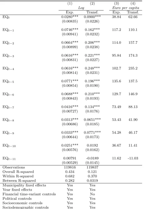
5.2 The role of grants
The role played by grants from upper-level governments in raising expenditure follow-ing an earthquake is summarized by the results reported in Table 3. Column 1 shows fixed effects estimates on the natural logarithm of per capita local government expendi-ture, and column 2 on the natural logarithm of per capita transfers. The coefficients of treatment variables are significant until the 10th year after the disaster for local govern-ment expenditure, similarly to the results obtained in Table 2, and until the 9th year for
31In the total population of municipalities, 19% of the treated municipalities are struck by an earthquake
with intensity equal to 6, and 4% with intensity > 7. In the matching sample, these percentages increase to 20% and 5%, respectively.
32
In 2017, an earthquake struck the isle of Ischia in the Campania region with a relatively low magnitude of 4, but caused relevant damages.
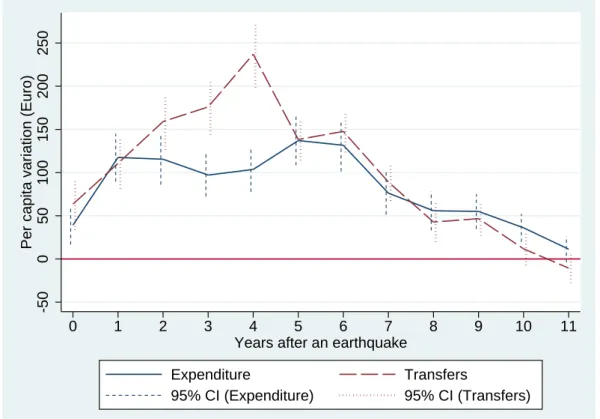
transfers. Moreover, transfers of financial resources grow initially faster than local govern-ment expenditure after an earthquake, and absolute per capita variations (in Euro) show that transfers increase more than expenditure between the 2nd and the 7th year after an event (see columns 3 and 4 of Table 3).33 This evidence is illustrated in Figure 4 with 95% confidence intervals. While the increase in per capita expenditure is roughly stable between the 2nd and the 6th year after an earthquake, transfers from central and regional governments follow a different trend. Central and regional governments tend to respond immediately to the higher spending requirements of treated municipalities. Then, from the 8th year after the event, additional transfers fall below the increase in expenditure. Overall, the increase in transfers overcomes the increase in expenditure.
Over the overall period (11 years), treated municipalities spend 952 Euro per individ-ual more than not affected municipalities, while per capita transfers are 1201 Euro higher. Hence, transfers of financial resources from central and regional governments seem to ex-ceed expenditure by 249 Euro per individual. If we consider that the average population of a treated municipality between 2000 and 2015 is about 10,000 individuals and 1129 mu-nicipalities are struck by an earthquake, the difference between transfers and expenditure amounts to almost 2.8 billion Euro. Generally, policy makers at central and regional levels allocate grants to municipalities affected by earthquakes mainly in the form of matching transfers. Although local governments are supposed to make use of these resources over time, some amount remains on hold and does not translate into higher expenditure for several years. Actually, an effective monitoring system on how resources are spent is still not in place, and transfers may also partially compensate lower revenues from local taxa-tion, since the central government can allow to postpone the payment of taxes for people residing in disaster areas.
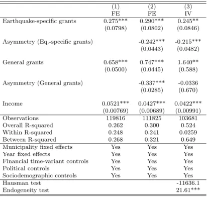
5.3 Flypaper effect and asymmetric response
The effects of earthquake-related grants (matching grants) and unconditional grants on local government spending are compared in Table 4. This table reports the results from fixed effects regressions using Equation 3. In column 1 the two asymmetry variables are initially excluded from the estimation. Note that both earthquake-specific and un-conditional grants stimulate expenditure more than income. The expenditure response
33
We transform the estimates of the treatment variables in columns 1 and 2 into real per capita variations usingAT Tˆ t−j = (1 − e− ˆαj)¯yt−j, with y identifying either per capita expenditure or per capita transfers
to one additional Euro of unmatching grants is almost 13 times larger than the response to income.34 Our estimated coefficient is slightly different from the coefficient estimated by Gennari and Messina (2014). This is because we use a fixed effects specification and data for a different period, and aggregate central and regional government transfers and current and capital transfers. However, our results are similar to the results obtained by Gamkhar and Oates (1996). Although the impact of matching grants is more than 5 times the effect of income, the multiplier is smaller than the multiplier of unconditional grants (about half). This is apparently surprising since the theory suggests that specific transfers should have at least the same effect on expenditure as unconditional transfers (Bailey and Connolly, 1998). However, as we will see later in Section 5.4, this is an average effect that does not account for heterogeneity in the response across the country, likely due to remarkable variation of efficiency in the use of earthquake-specific transfers.
In column 2, we extend the model to include the two asymmetry variables that capture different effects between increasing and decreasing transfers. The negative and significant coefficient of the asymmetry variable relative to unconditional grants suggests that there is a replacement effect when transfers decrease, i.e., expenditure is sticky to decreasing unconditional grants, a result in line with the findings of Gennari and Messina (2014). Sim-ilarly, expenditure is less responsive to decreasing than to increasing earthquake-specific grants, although this asymmetric response is more pronounced than the response to un-conditional transfers. The sum of the estimated parameters of earthquake-specific grants ( ˆα1) and their asymmetry variable ( ˆα2) is close to zero and suggests that a reduction in the transfers for earthquake recovery has negligible effects on spending levels.
In column 3, we report the results from the estimation of a 2SLS fixed effects regression instrumenting general transfers and the relative asymmetry variable with the second lag of general transfers and the second lag of general transfers of neighboring municipalities (2-years spatial lag).35 Diagnostic tests confirm that general transfers are endogenous and that the instrumental variable approach yields consistent estimates. We can see that the effect of general grants on spending levels is more remarkable than in column 1 and 2, and the coefficient of the asymmetric response to decreasing grants loses significance. These coefficients are very close to the estimates of Gennari and Messina (2014). Conversely, the
34The coefficient of unmatching grants does not change if we estimate Equation 3 using only the
sub-sample of municipalities not affected by earthquakes.
35To enhance the comparability of our results with those obtained by Gennari and Messina (2014),
we repeat the estimation using the first and the second temporal lag of transfers, but differences are insignificant.
estimated parameters of earthquake-specific grants and their asymmetry variable are very close to the coefficients reported in column 2. Overall, these results allow to conclude that there is evidence of flypaper effect for both types of grants. However, we find inconclusive evidence of an asymmetric response to increasing vs. decreasing unconditional transfers (fiscal replacement), similarly to most previous studies but differently, for instance, from Levaggi and Zanola (2003), who testify a fiscal restraint type of asymmetry on regional health care expenditure in Italy. Conversely, the fiscal replacement effect is remarkable for earthquake-specific matching grants, suggesting that public officials may exploit the oc-currence of earthquakes to maintain higher spending levels. Moreover, local governments are apparently unable to fully exploit upper-level government transfers to increase expen-diture when struck by an earthquake. This suggests a delay in the response to increasing grants, leading to an inefficient use of resources for disaster relief. We further address this aspect in the next Section 5.4.
5.4 The North-South divide 5.4.1 Timing of the response
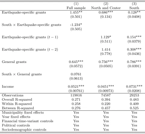
Local governments may differ in the response to earthquake recovery measures. Sev-eral aspects, such as culture, history and institutional quality, may affect this response. Barone and Mocetti (2014) argue that these differences influence economic outcomes af-ter an earthquake. They compare two big earthquakes in Italy and show that the lower institutional quality in the South worsened after the shock and led to a lower economic growth (for a discussion on the regional divide in Italy, see for instance Felice (2018) and Gonz´alez (2011)). Following this evidence and inspired by the above findings on asymmet-ric and heterogeneous flypaper effects, we analyze how the response of local governments to earthquake shocks differs between Northern an Southern municipalities. The results from the estimation of the extended Equation 3 to include the interaction terms between grants and location are reported in Table 5.
As for unconditional grants, we do not observe a significantly different effect be-tween Northern and Southern municipalities (in column 1, the coefficient of the inter-action term between the South dummy and unconditional grants is not significant). Con-versely, earthquake-specific grants show a significantly different effect between Northern and Southern municipalities. In the North, one additional Euro of transfers for earthquake recovery raises expenditure by 1.43 Euro, while in the South the effect is significantly lower
(0.22 Euro, i.e., the sum of the coefficient of earthquake-specific grants and the interaction term). Therefore, municipalities in the North seem to overreact to transfers for earthquake recovery, while expenditure in the South is much more sticky. Note that Northern munici-palities are generally less dependent on transfers and their spending levels are lower, which may suggest a lower inertia to changes in transfers. Also, the slower use of earthquake-related resources by municipalities in the South may be the consequence of higher levels of corruption (Mauro, 1995).
The possible delay in the utilization of earthquake-related funds is worth of further analysis. The model in columns 2 and 3 includes the first and second lag of earthquake-specific grants and runs separate regressions for Northern and Southern municipalities. In the North, the inclusion of past matching grants in the regression reduces the estimated coefficient of current-period grants below 1, while the coefficient of the first lag is significant and equal to 1.1, and the coefficient of the second lag is not significant. This suggests that Northern local governments have at most one-year delay in the reaction to additional resources from upper-level governments. Instead, in the South, the immediate response to matching grants is lower (0.128 vs. 0.686), and both the first and the second lag of grants are significant. Moreover, both lag coefficients are below 1 and lower than the estimated coefficients for the North, suggesting that a larger amount of financial resources received by local governments is not spent in the short-run. This may indicate that municipalities in the South are affected by poorer institutional quality, which in turn may cause only partial or delayed recovery from earthquake damages and hinder local economic growth in the future.
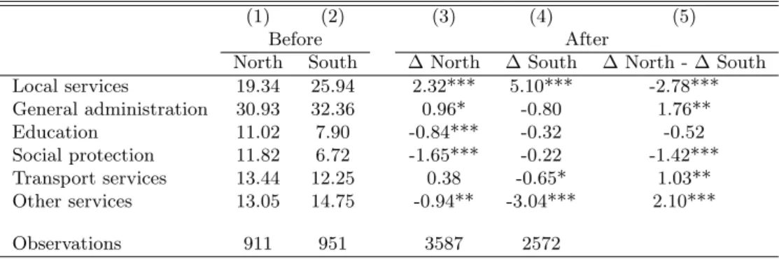
5.4.2 Spending composition and growth
To further explore possible inefficiencies in local government response to earthquake shocks, we analyze how disaster relief resources are allocated to different spending cate-gories. In Table 6, we compare variations in the spending composition between munic-ipalities in the North and in the South in the 5 years before and after the occurrence of an earthquake.36,37 Before the shock, municipalities in the South spend on average 25.9% of the total budget on local services, which exceeds by 6.6% the budget allocated
36The spending category Other includes local police, justice, culture, sports and economic development
which aggregated account on average for less than 10% of the total budget.
37Table 6 in the Appendix reports variations before and after the shock and between municipalities in
by municipalities in the North. Not surprisingly, after the shock, the expenditure share of local services grows in both macro regions since it includes expenditure on public infras-tructures, water supply and waste disposal. More precisely, municipalities in the North allocate 2.32% and 0.96% significantly more resources to local services and administra-tion, respectively, while the budget share for the other spending categories significantly decreases, except for transport services. Instead, the share allocated to local services by Southern municipalities increases by 5.1%, which goes to the detriment of the budget share allocated to the other spending categories (a significant decrease for transport ser-vices and other serser-vices). Therefore, the main difference in the spending composition between Northern and Southern municipalities lies in the remarkable increase of funds for local services in the South, and a relatively more equal allocation of resources across spending categories in the North. While the response of local governments to earthquake shocks in Northern municipalities encompasses all areas of government action, Southern municipalities put their effort mainly in the enhancement of local services.
The heterogeneous response to earthquake shocks observed between the North and the South in terms of timing in the use of resources and their allocation points at the most efficient recovery from earthquake shocks. Therefore, we relate the availability and allocation of earthquake-specific resources to economic growth and compare treated and matched unaffected municipalities in the North and in the South.38 We use personal income and mean housing prices as proxies for local economic growth since data on gross domestic product (GDP) are not available at municipality level.39 The trends of these variables are illustrated in Figure 5. Note that, in the North, personal income grows faster in struck municipalities than in unaffected municipalities in the first decade after an earthquake (Figure 5a). Conversely, in the South, the two groups of municipalities have identical income trends (Figure 5b). Similarly, housing prices (per square meter) in the South do not change significantly between struck and unaffected municipalities (Figure 5d). Instead, in the North, housing prices start to grow faster after 4 years in struck municipalities as compared to unaffected municipalities (Figure 5c). This evidence is even more pronounced if we limit the focus to earthquakes with intensity equal or greater than 6. It appears that the result is related to different responses to earthquake shocks between
38In this part of the analysis we exclude municipalities from the region Abruzzo because the 2009
earthquake that affected this region is an outlying shock with strong damages and large financial windfall for reconstruction from upper-tier governments.
39
See, for instance, Cheung et al. (2018) and Naoi et al. (2009) for an examination of the effects of earthquakes in terms of house and land values.
municipalities in the two macro-regions. Transfers from central and regional governments in the North (Figure 6a) grow after the occurrence of an earthquake, but converge to pre-earthquake levels after 6 years. Conversely, in the South, struck municipalities remain persistently more dependent on upper-tier government transfers for at least 10 years (see Figure 6b) and allocate a large share of additional resources to local services (Figure 6c and 6d).
This evidence obtained from the large dataset of all Italian municipalities and earth-quake events between 2000 and 2015, seems to confirm the heterogeneous effects between North and South found by Barone and Mocetti (2014) in their deep investigation of two Italian earthquakes. Even if a larger amount of resources for recovery is allocated to dis-aster areas in the South, these jurisdictions seem unable to exploit the financial windfall to recover from damages and improve economic growth. Conversely, local governments in the North appear more efficient in exploiting transfers from upper-level governments to expand expenditure and recover from damages. This translates into new infrastructure and the replacement of obsolete technologies destroyed or damaged by the earthquake, which allows to foster local economic development and to accelerate growth. Likely, the allocation of resources among spending categories in the North speeds up recovery and fosters local economic growth. The higher increase in the expenditure share for local ser-vices in the South could suggest that resources are not used efficiently or favor corruption. Indeed, although local services represents the spending category mostly affected by earth-quakes (urban road maintenance and the maintenance/construction of public buildings), the construction industry is also well exposed to corruption scandals.
6
Concluding remarks
Local governments differ in the response to economic and social damages caused by natural disasters (earthquakes), in terms of spending behavior and the use of grants from upper tiers. Earthquake-related grants (matching grants) may also differ from other types of grants (mostly unconditional) in terms of stimulatory power, and expenditure may differ in the response to increasing and decreasing grants, leading to asymmetric and heterogeneous reactions (different flypaper effects). We explore these differences using municipality data and all earthquake shocks from a country largely exposed to seismic events - Italy - between 2000 and 2015.