Bridging adaptive estimation and control with modern machine learning : a quorum sensing inspired algorithm for dynamic clustering

Bridging Adaptive Estimation and Control with

Modern Machine Learning:

A Quorum Sensing

Inspired Algorithm for Dynamic Clustering

by

Feng Tan

Submitted to the Department of Mechanical Engineering

in partial fulfillment of the requirements for the degree of

Master of Science in Mechanical Engineering

at the

MASSACHUSETTS INSTITUTE OF TECHNOLOGY "_L

September 2012

@

Massachusetts Institute of Technology 2012. All rights reserved.

Author ...

Department of Mechanical Engineering

August 20, 2012

OCT 2 2 2012

RARIES

Certified by...

...

7Th

/

.-... . . ..

Jean-Jacques Slotine

Professor

Thesis Supervisor

Accepted by ...

David E. Hardt

Chairman, Department Committee on Graduate Students

Bridging Adaptive Estimation and Control with Modern

Machine Learning: A Quorum Sensing Inspired Algorithm

for Dynamic Clustering

by

Feng Tan

Submitted to the Department of Mechanical Engineering on August 30, 2012, in partial fulfillment of the

requirements for the degree of

Master of Science in Mechanical Engineering

Abstract

Quorum sensing is a decentralized biological process, by which a community of bac-terial cells with no global awareness can coordinate their functional behaviors based only on local decision and cell-medium interaction. This thesis draws inspiration from quorum sensing to study the data clustering problem, in both the time-invariant and the time-varying cases.

Borrowing ideas from both adaptive estimation and control, and modern machine learning, we propose an algorithm to estimate an "influence radius" for each cell that represents a single data, which is similar to a kernel tuning process in classical machine learning. Then we utilize the knowledge of local connectivity and neighborhood to cluster data into multiple colonies simultaneously. The entire process consists of two steps: first, the algorithm spots sparsely distributed "core cells" and determines for each cell its influence radius; then, associated "influence molecules" are secreted from the core cells and diffuse into the whole environment. The density distribution in the environment eventually determines the colony associated with each cell. We integrate the two steps into a dynamic process, which gives the algorithm flexibility for problems with time-varying data, such as dynamic grouping of swarms of robots. Finally, we demonstrate the algorithm on several applications, including bench-marks dataset testing, alleles information matching, and dynamic system grouping and identication. We hope our algorithm can shed light on the idea that biological inspiration can help design computational algorithms, as it provides a natural bond bridging adaptive estimation and control with modern machine learning.

Thesis Supervisor: Jean-Jacques Slotine Title: Professor

Acknowledgments

I would like to thank my advisor, Professor Jean-Jacques Slotine with my sincerest

gratitude. During the past two years, I have learned not only knowledge, but also principles of doing research under his guidance. His attitude to a valuable research topic, "Simple, and conceptually new", although sometimes "frustrating", is inspiring me all the time. His broad vision and detailed advice help me all the way towards novel and interesting explorations. He is a treasure to any student and it has been a honor to work with him.

I would also like to thank my parents for unwavering support and encouragement. All the time from childhood, my curiosity and creativity were so encouraged and my

interests were developed with their support. I feel peaceful and warm with them on my side as always.

Contents

1 Introduction 1.1 Road Map ... 1.2 M otivations . . . . 1.2.1 Backgrounds. . . . . 1.2.2 Potential Applications . . . . .

1.2.3 Goal of this thesis . . . . 1.3 Clustering Algorithms . . . . 1.3.1 Previous Work . . . . 1.3.2 Limitations of Current Classical 1.4 Inspirations from Nature . . . . 1.4.1 Swarm Intelligence . . . . 1.4.2 Quorum Sensing . . . . 13 14 . . . . 15 . . . . 15 . . . . 16 . . . . 17 . . . . 17 . . . . 18 Clustering Techniques . . . . 23 . . . . 24 . . . . 25 . . . . 26

2 Algorithm Inspired by Quorum Sensing 2.1 Dynamic Model of Quorum Sensing . . . . 2.1.1 Gaussian Distributed Density Diffusion . 2.1.2 Local Decision for Diffusion Radius . . . 2.1.3 Colony Establishments and Interactions 2.1.4 Colony Merging and Splitting . . . . 2.1.5 Clustering Result . . . . 2.2 Mathematical Analysis . . . . 2.2.1 Convergence of Diffusion Tuning . . . . . 2.2.2 Colony Interaction Analysis . . . . 29 . . . . 29 . . . . 31 . . . . 33 . . . . 35 . . . . 36 . . . . 37 . . . . 39 . . . . 39 . . . . 43

2.2.3

Analogy to Other Algorithms . . . .4

3 Experimental Applications 3.1 Synthetic Benchmarks Experiments . . . . 3.2 Real Benchmarks Experiments . . . . 3.3 Novel Experiment on Application for Alleles Clustering 3.4 Experiments on Dynamic System Grouping . . . . 3.4.1 M otivation . . . . 3.4.2 Application I. Clustering of mobile robots . . . 3.4.3 Application II. Clustering of adaptive systems . 3.4.4 Application III. Multi-model switching . . . . . 4 Conclusions 4.1 Summary . . . . 4.2 Future Work. . . . . 49 . . . . 49 . . . . 56 . . . . 59 . . . . 70 . . . . 71 . . . . 72 . . . . 75 . . . . 79

83

83

86

46

List of Figures

1-1 Quorum sensing model . . . . 2-1 The interactions between two colonies . . . .

3-1 3-2 3-3 3-4 3-5 3-6 3-7 3-8 3-9 3-10 3-11 3-12 3-13 3-14 3-15 3-16 3-17 3-18 3-19

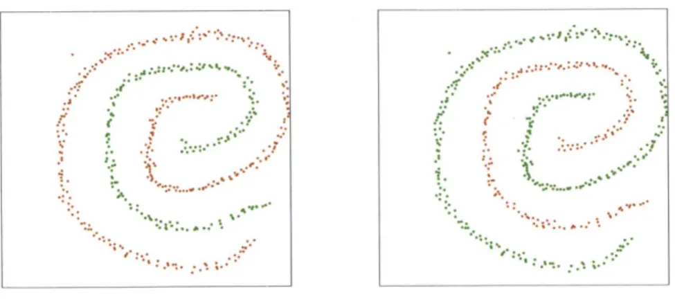
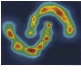
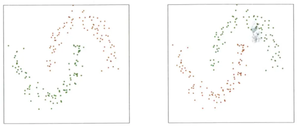
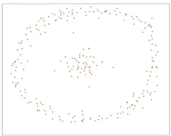
The two-chain shaped data model . . . . Density distribution of two-chain shaped data model Clustering result of the two-chain shaped data model The two-spiral shaped data model . . . . Density distribution of two-spiral shaped data model Clustering result of the two-spiral shaped data model The two-moon shaped data model . . . . Density distribution of two-moon shaped data model Clustering result of the two-moon shaped data model The island shaped data model . . . . Density distribution of island shaped data model . . . . Clustering result of the island shaped data model . . . The clustering result of Iris dataset . . . . The distribution map of data and density in 14 seconds Variation of density and influence radius of a single cell Cluster numbers of over the simulation time . . . . Initial parameters configuration of the 60 systems . . . Cluster numbers during the simulation . . . . Parameter estimations of the real system . . . . 3-20 Density of the real system

27 46 . . . . 50 . . . . 50 . . . . 51 . . . . 51 . . . . 52 . . . . 52 . . . . 53 . . . . 53 . . . . 54 . . . . 55 . . . . 55 . . . . 56 . . . . 57 . . . . 73 . . . . 74 . . . . 74 . . . . 78 . . . . 78 . . . . 80 . . . . 8 0

3-21 Trajectory of the real system . . . . 81 3-22 Error of the real system . . . . 81

List of Tables

3.1 Clustering result of Pendigits dataset . . . . 58

3.2 Clustering result comparison with NCut, NJW and PIC . . . . 59

3.3 Clustering result of the alleles data . . . . 61

3.4 Clustering result match-up of alleles clustering . . . . 70

Chapter 1

Introduction

This thesis is primarily concerned with developing an algorithm that can bridge adap-tive estimation and control with modern machine learning techniques. For the specific problem, we develop an algorithm inspired by nature, dynamically grouping and co-ordinating swarms of dynamic systems. One motivation of this topic is that, we will inevitably encounter control problems for groups or swarms of dynamic systems, such as manipulators, robots or basic oscilators, as researches in robotics advance. Conse-quently, incorporating current machine learning techniques into the control theory of groups of dynamic systems would enhance the performance and achieve better results

by forming "swarm intelligence". This concept of swarm intelligence would be more

intriguing if the computation can be decentralized and decisions can be made locally since such mechanism would be more flexible, consistent and also robust. With no central processor, computational load can be distrbuted to local computing units, which is both efficient and reconfigurable.

When talking about self-organization and group behavior, in control theory we have the ideas about synchronization and contraction analysis, while in the machine learning fields, we can track the progress in a lot of researches in both supervised or un-supervised learning. Currently researches are experimenting with various methods on classification and clustering problems, such as Support Vector Machine[1], K-Means clustering[2], Spectral clustering[3] [4], etc. However, rarely have these algorithms been developed to fit into the problems of controling retime dynamic systems,

al-though successful applications in image processing, video and audio recognition have

thrived in the past decades.

The main challenge that we will consider in this thesis is how to modify and

fomulate the current machine learning algorithms, so that they can fit in and improve

the control performance of dynamic systems. The main contribution of this thesis

is that we develop a clustering algorithm inspired by a natural phenomenon-quorum

sensing, that is able to not only perform clustering on benchmark datasets as well

as or even better than some existing algorithms, but also integrate dynamic systems

and control strategies more easily. With further extensions made possible through

this integration, control theory would be more intelligent and flexible. With the

inspiration from nature, we would like to discuss more about the basic concepts

like what is neighborhood, and how to determine the relative distance between data

points. We hope these ideas provide machine learning with deeper understandings

and also find the unity between control, machine learning and nature.

1.1

Road Map

The format in Chapter 1 is as follows: we will first introduce the motivations of

this thesis, with backgrounds, potential applications and detailed goal of this thesis.

Then we will briefly introduce the clustering alogorithms by their characteristics and

limitations. Finally, we will illustrate our inspiration from nature, with detailed

description of quorum sensing and the key factors of this phenomenon that we can

extract to utilize for developing the algorithm.

Beyond the current chapter, we will describe detail analysis of our algorithm in the

second chapter. We will provide mathematical analysis on the algorithm from both

views from machine learning and dynamic system control stability. Then clustering

merging and splitting policies will be introduced along with comparison with other

clustering algorithms. In chapter three, we will put our clustering algorithm into

actual experiments, including both synthetic and real benchmarks experiments,

ex-periments on alleles classification, and finally on real time dynamic system grouping.

In the last chapter, we will discuss about the results shown in the previous chapters

by comparing the strengths and weaknesses of our proposed algorithm, and provide

our vision on future works and extensions.

1.2

Motivations

Control theory and machine learning share the same goal, which is to optimize certain functions to either reach a minimum/maxmimum or track a certain trajectory. It is the implementing methods that differs the two fields. In control theory, since the controled objects have the requirements of real-time optimization and stability, the designed control strategy starts from derivative equations, so that after a period of transient time, satisfying control performance can be achieved. On the other hand, machine learning faces mostly with static data or time varying data where a static feature vector can be extracted from, so optimization in machine learning is more direct to the goal by using advanced mathematical tools. We think if we can find a bridge connecting the two fields more closely, we can then utilize the knowledge learned from past to gain better control performance, and also we can bring in the concepts like synchronization, contraction analysis, and stability into

machine learning theories.

1.2.1

Backgrounds

Research in adaptive control started in early 1950's as a technology for automatically adjusting the controller parameters for the design of autopilots for aircrafts[5]. Be-tween 1960 and 1970 many fundamental areas in control theory such as state space and stability theory were developed. These progresses along with some other tech-niques including: dual control theory, identification and parameter estimation, helped scientists develop increased understanding of adaptive control theory. In 1970s and 1980s, the convergence proofs for adaptive control were developed. It was at that time a coherent theory of adaptive control was formed, using various tools from nonlinear control theory. Also in the early 1980s, personal computers with 16-bit

microproces-sors, high-level programming languages and process interface came on the market.

A lot of applications including robotics, chemical process, power systems, aircraft

control, etc. benefitting from the combination of adaptive control theory and com-putation power, emerged and changed the world.

Nowadays, with the development of computer science, computation power has been increasing rapidly to make high-speed computation more accessible and inex-pensive. Available computation speed is about 220 times what it was in the 1980's when key adaptive control techniques were developed. Machine learning, whose ma-jor advances have been made since the early 2000s, benefitted from the exploding computation power, and mushroomed with promising theory and applications. Con-sequently, we start looking into this possibility of bridging the gap between machine learning and control, so that the fruit of computation improvements can be utilized and transferred into control theory for better performance.

1.2.2

Potential Applications

Many potential applications would emerge if we can bridge control and machine learn-ing smoothly, since such a combination will give traditional control "memory", in-telligence and much more flexibility. By bringing in manifold learning into control, which is meant to find a low dimentional basis for describing high dimentional data, we can possibly develop an algorithm that can shrink the state space into a much smaller subset. High dimensional adaptive controllers, especially networks controllers like[6] would benefit hugely from this. Also we can use virtual systems along with dynamic clustering or classification analysis to improve performance of multi-model switching controllers, such as [7] [8][9] [10]. This kind of classification technique would also be helpful for diagnosis of control status, such as anonaly detections in [11]. Our effort presented in developing a clustering algorithm that can be incorporated with dynamic systems is a firm step right on building this bridge.

1.2.3

Goal of this thesis

The goal of this thesis is to develop a dynamic clustering algorithm suitable to imple-ment on dynamic systems grouping. We propose this algorithm with better clustering performances on static benchmarks datasets compared to traditional clustering meth-ods. In the algorithm, we would like to realized the optimization process not by direct mathematical analysis or designed iterative steps, yet by derivative equations conver-gence, since such algorithm would be easily combined with contraction analysis or control stability analysis for coordinating group behavior. We want to develop the algorithm not so "artificial", yet in a more natural view.

1.3

Clustering Algorithms

When thinking about the concept of intelligence, two basic parts contributing to in-telligence are learning and recognition. Robots, who can calculate millions of times faster that human, are good at conducting repetitive tasks. Yet, they can hardly function when faced with a task that has not been predefined. Learning and recog-nition requires the ability to process the incoming information, conceptualize it and finally come to a conclusion that can describe or represent the characteristics of the

perceived object or some abstract concepts. The concluding process requires to de-fine the similarities and dissimilarities between classes, so that we can distinguish one from another. In our mind we put things that are similar to each other into a same groups, and when encountering new things with similar charateristics, we can recognize them and classify them into these groups. Furthermore, we are able to rely -on the previously learned knowledge to make future predictions and guide future behaviors. Thus, it is reasonable to say, this clustering process, is a key part of the learning, and further a base of intelligence.

Cluster analysis is to separate a set of unlabeled objects into clusters, so that the ob-jects in the same cluster are more similar, and obob-jects belonging to different clusters are less similar, or dissimilar. Here is a mathematical description of hard clustering problein[12]:

Given a set of input data X = ₁

,x

₂

,x

₃

,

... N,

Partition the data into K groups:

C1, C2, C3, ...CK,

(K

;

N), such that

1) Ci

#

0,

i = 1,

2,

..., K;

K

2) U Ci = X;

3)

Ci

(~

Cy

= 0,

i, j

=

1, 2,7... K, i

# j

Cluster analysis is widely applied in many fields, such as machine learning, pattern

recognition, bioinformatics, and image processing. Currently, there are various

clus-tering algorithms mainly in the categories of hierarchical clusclus-tering, centroid-based

clustering, distribution-based clustering, density-based clustering, spectral clustering,

etc. We will introduce some of these clustering methods in the following part.

1.3.1

Previous Work

Hierarchical clustering

There are two types of hierarchical clustering, one is a bottom up approach, also

know as "Agglomerative", which starts from the state that every single data forms

its own cluster and merges the small clusters as the hierarchy moves up; the other

is a top down approach, also know as "Divisive", which starts from only one whole

cluster and splits recursively as the hierarchy moves down. The hierarchical

clus-tering algorithms intends to connect "objects" to "clusters" based on their

dis-tance. A general agglomerative clustering algorithm can be summarized as below:

1. Start with N singleton clusters.

Calculate the proximity matrix for the N clusters.

2. Search the minimal distance

D(Ci, C₃) = min1<m, 1N,1mD(Cm,

C

1)

Then combine cluster Ci, Cj to form a new cluster. 3. Update the proximity matrix.

4. Repeat step 2 and 3.

However, the hierarchical clustering algorithms are most likely sensitive to outliers and noise. And once a misclassification happens, the algorithm is not capable of correcting the mistake in the future. Also, the computational complexity for most of hierarchical clustering algorithms is at least O(N 2). Typical examples of hierarchical

algorithms include CURE[13], ROCK[14], Chameleon[15], and BIRCH[16].

Centroid-based clustering

The Centroid-based clustering algorithms try to find a centroid vector to represent a cluster, although this centroid may not be a member of the dataset. The rule to find this centroid is to optimize a certain cost function, while on the other hand, the be-longings of the data are updated as the centroid is repetitively updated. K-means[2] clustering is the most typical and popular algorithm in this category. The algorithm partition n data into k clusters in which each data belongs to the cluster with the nearest mean. Although the computation is NP-hard, there are heuristic algorithms that can assure convergence to a local optimum.

The mathematical model of K-means clustering is:

Given a set of input data X - _Y2, 1, X ₃, ...XN, Partition them into k sets C1, ... CK, (K <

N), so as to minimize the within cluster sum of squares:

k

argmirnc

S(

|x- ti||2

i=1 xjGCi

where pi is the mean of points in Ci

Generally, the algorithm proceeds by alternating between two steps:

Update step: calculate the new means m =Ct) -- 1

xjEC~t)

However, the K-means algorithm has several disadvantages. It is sensitive to initial

states, outliers and noise. Also, it may be trapped in a local optimum where the

clustering result is not acceptable. Moreover, it is most effective working on

hyper-spherical datasets, when faced with some dataset with concave structure, the centroid

information may be not precise or even misleading.

Distribution-based clustering

Distribution based clustering methods are closely related to statistics. They tend to

define clusters using some distribution candidates and gradually tune the

parame-ters of the functions to fit the data better. They are especially suitable for artificial

datasets, since they are originally generated from a predefined distribution. The most

notable algorithm in this category is expectation-maximization algorithm. It assumes

that the dataset is following the a mixture of Gaussian distributions. So the goal of

the algorithm is to find the mutual match of the Gaussian models and the actual

dataset distribution.

Given a statistical model consisting of known data X =1, 2, X₃, ...XN,, latent data

Z, and unknown parameters

0,

along with the likelihood function:

L(; X, Z) = p(X, Z|0)

and the marginal likelihood

L(O; X) = p(XI) =

(Zp(X,

Z|0

Z

The expectation-maximization algorithm then iteratively applies the following two

steps:

Expectation step: calculate the expected value of log likelihood function

Maximization step: Find the parameter to maximize the expectation

W'+) = argmarg.Q( I9(t)

However, the expectation-maximization algorithm is also very sensitive to the initial selection of parameters. It also suffers from the possibility of converging to a local optimum and the slow convergence rate.

Density-based clustering

Density based lustering algorithms define clusters as areas of higher density than the remainder area. The low density areas are most likely to be bonders or noise region. In this way, the algorithm should handle the noise and outliers quite well since their relevant density should be too low to pass a threshold. The most popular density based algorithm is DBSCAN[17)(for density-based spatial clustering of applications with noise). DBSCAN defines a cluster based on "density reachability": a point q is directly density-reachable from point p if distance between p and q is no larger that a given radius E. Further if p is surrounded by sufficiently many points, one may consider the two points in a cluster. So the algorithm requires two parameters: e and the minimum of points to form a cluster (minPts). Then the algorithm can start from any random point measuring the c neighborhood. The pseudo-code of the algorithm is presented below:

DBSCAN(D, e, MinPts)

C = 0

for each unvisited point P in dataset D mark P as visited

NeighborPts = regionQuery(P, 6)

if sizeof (NeighborPts) < MinPts mark P as NOISE

else

C = nextcluster

add P to cluster C

for each point P' in NeighborPts

if P' is not visited

mark P' as visited

NeighborPts' = regionQuery(P', E) if sizeof (NeighborPts') >= MinPts

Neighbor Pts = NeighborPts joined with NeighborPts'

if P' is not yet member of any cluster

add P' to cluster C

regionQuery(P,

e)

return all points within P's e-neighborhood

It is good for the DBSCAN that it requires no specific cluster number information

and can find arbitrarily shaped clusters. It handles outliers and noise quite well.

However, it depends highly on the distance measure and fails to cluster datasets with

large differences in densities. Actually, by using a predefined reachability radius, the

algorithm is not flexible enough. Also, it relies on some kind of density drop to detect

cluster borders and it can not detect intrinsic cluster structures.

Spectral clustering

Spectral clustering techniques use the spectrum(eigenvalues) of the proximity matrix

to perform dimensionality reduction to the datasets. One prominent algorithm of this

category is Normalized Cuts algorithm[4], commonly used for image segmentation.

We will introduce the mathematical model of the algorithm below:

Let G

=

_{(V, E) be a weighted graph, and A and B as two subgroups of the vertices.}

AUB =V,AfB =0

cut(A, B)

=

E

w(u, v)

uEA,vEB

assoc(A, V)

=

E

w(u, t) and assoc(B, V)=

Z

w(v, t)

uEA,tEV vEB,tEV

then Ncut(A, B)

= cut(A,B) + cut(B,A)

Let d(i) = wi and D be an n x n diagonal matrix with d on the diagonal, then

after some algebric manipulations, we get

minANcut(A, B)

=

ming V ,

where

yJ E {1, -b} for some constant b, and yfD1 = 0

To minimize g (-W, and avoid the NP-hard problem by relaxing the constraints

on g, the relaxed problem is to solve the eigenvalue problem (D - W)g = AD' for

the second smallest generalized eigenvalue.

And finally bipartition the graph according to this second smallest eigenvalue.

The algorithm has solid mathematical background. However, calculating the eigen-values and eigenvectors takes lots of computation. Especially if there are some tiny

fluctuations in the data along time, the whole calculating process must be redone all over again, which makes calculations in the past useless.

1.3.2

Limitations of Current Classical Clustering Techniques

With the introduction and analysis on current existing clustering algorithms, we can conclude with some limitations of current classical clustering techniques:

1. Many algorithms require the input of cluster number. This is acceptable when

the data is already well known, however, a huge problem otherwise. 2. The sensitivity to outliers and noise often influences the clustering results.

3. Some of the current algorithms can not adapt to clusters with different density

or clusters with arbitrary shape.

4. Almost all algorithms adopt pure mathematical analysis, that are infeasible to be combined with dynamic systems and control theory. The lack of time dimen-sion makes most of the algorithms a "one-time-deal", of which past calculations can not provide reference to future computations.

Actually, there are many examples in nature, like herds of animals, flocks of birds, schools of fish and colonies of bacteria, that seem to deal quite well with those

prob-lems. The robustness and flexibility of natural clusters far exceed our artificial algo-rithms. Consequently, it is natural to take a look at the nature to look for inspirations of a new algorithm that handles those problems well.

1.4

Inspirations from Nature

Nature is a great resource to take a look at when we want to find a bridge between computational algorithms and dynamic systems. On one hand, a lot of biological behaviors themselves are intrinsically dynamic systems. We can model these biologi-cal behaviors into physibiologi-cal relations and moreover into dynamic equations. Actually, many biomimic techniques such as sonar technology and flapping aircrafts are devel-oped following this path. The close bonding between biology behaviors and dynamic systems makes it possible to not only simulate biology processes through dynamic models, but also control such processes toward a desired goal or result. Thus, it would be highly possible to develop control algorithms for biomimic systems in a biological sense, which is able to achieve efficient, accurate and flexible control performance.

On the other hand, computer science has been benefitting from learning from the nature for a long history. Similar mechanisms and requirements are shared by computational science and biology, which provide a base for cultivating various joint applications related to coordination, network analysis, tracking, vision and etc.[181. Neuro networks[19][20], which has been broadly applied and examined in machine learning applications such as image segmentation, pattern recognition and even robot control, is a convincing example derived from ideas about the activities of neurons in the brain; Genetic algorithms[21], which is a search heuristic mimics the process of natural evolution, such as inheritance, mutation, selection, and crossover, have been widely applied over the last 20 years. Also, there have been many valuable researches motivated by the inspirations of social behaviors existing among social insects and particle swarms, which we will discuss in details in the following section 1.4.1.

There are several principles of biological systems that make it a perfect bridge con-necting dynamic system control and machine learning algorithms[18]. First, dynamic

systems require real-time control strategy, which most modern machine learning algo-rithns fail to meet because that advanced and resource-demanding mathmetical tools are involved. However, a machine learning algorithm inspired by biology process is most likely to be feasible to be converted into a dynamically evolving process, such as ant colony algorithms and simulated annealing algorithms. Secondly, biological pro-cesses need to be able to handle failures and attacks successfully in order to survive and thrive. This property shares the same or similar concept with the robustness requirements for computation algorithms and also stability and resistance to noise for dynamic systems control strategy. So we may use the biological bridge connecting these properties in different fields and complement them with each other. Thirdly, biological processes are mostly distributed systems, such as molecules, cells, or or-ganisms. The interaction, coordination, among the agents along with local decisions make each agent not only an information processing unit, but also a dynamic unit. This is very promising for connecting information techniques with dynamic control, and also for bringing in more intelligence into mechanical engineering field.

These shared principles indicate that bridging dynamic system control with ma-chine learning through biology inpired algorithms is very promising. Such connection may improve understanding in both fields. Especially, the computational algorithms focus on speed, which requires utilizing advanced mathematical tools, but simultane-ously makes the algorithm less flexible to time varying changes from both data side and environments. Since biological systems can inherently adapt to changing envi-ronments and constrains, and also they are able to make local decisions with limited knowledge, yet optimize towards a global goal, they are ideal examples to learn from for machine learning algorithm to realize large scale self organizing learning. In the following section 1.4.1, we will introduce some previous work utilizing this fact for

building swarm intelligence.

1.4.1

Swarm Intelligence

Swarm intelligence is a mechanism that natural or artificial systems composed of many individuals behave in a collective, decentralized and self-organized way. In swarm

intelligence systems, a population of simple agents interact locally with each other and with the environment. Although there is no centralized control structure dictating individual behavior, local interactions between the agents lead to the emergence of global intelligent behavior. This kind of simple local decision policy hugely reduces the computational load on each information processing unit. Such mechanism pervades in nature, including social insects, bird flocking, animal herding, bacterial growth, fish schooling, and etc. Many scientific and engineering swarm intelligence studies emerge in the fields of clustering behavior of ants, nest building behavior of termites, flocking and schooling in birds and fish, ant colony optimization, particle swarm optimization, swarm-based network management, cooperative behavior in swarms of robots, and so on. And various computational algorithms have been inspired by the facts. For the swarm intelligence algorithms, we now have: Altruism algorithm[22],

Ant colony optimization [23], Artificial bee colony algorithm[24], Bat algorithm[25], Firefly Algorithm[25], Particle swarm optimization [26], Krill Herd Algorithm[27], and

so on.

The natural inspiration that we take in this thesis is Quorum Sensing, which will be described in details in section 1.4.2.

1.4.2

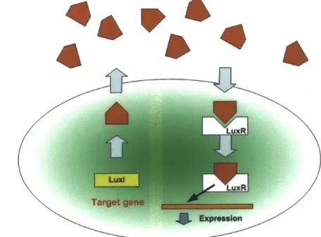
Quorum Sensing

Quorum Sensing[28] [29][30][31] [32] [33][34][35] is a biological process, by which a

com-munity of bacteria cells interact and coordinate with their neighboring cells locally with no awareness of global information. This kind of local interaction is not achieved through direct cell-to-cell communication. Actually, each cell sends out signaling molecules called autoinducers that diffuse in the local environment and builds up local concentration. These auto inducers that carry introduction information can be captured by the receptors, who can activate transcription of certain genes that are equipped in the cell. In V. fisheri cells, the receptor is LuxR. There is a low likelihood of a bacterium detecting its own secreted inducer. When only a few cells of the same kind are present in the neighborhood, diffusion can reduce the density of the induc-ers to a low level, so that no functional behavior will be initiated, which is "energy

efficient". However, when the concentration of the surrounding area reaches a

thresh-old, more and more inducers will be synthesized and trigger a positive feedback loop,

to fully activate the receptors. Almost at the same time, specific genes begin being

trascripted in all the cells in the local colony, and the function or behavior expressed

by the genes will be performed collectively and coordinatedly in the swarm. For

in-stance, if only one single Vibrio fischeri exists in the enviroment, then producing the

bioluminescent luciferase would be a waste of energy. However when a quorum in

vicinity is confirmed, such collective production can be useful and functional. Fig.1-1

gives a pictorial view of the process in Vibrio fischeri.

LuxR

Figure 1-1: Quorum sensing model

In this context, quorum sensing is applicable in developing clustering algorithms,

since the cells can sense when they are surrounded in a colony by measuring the

autoinducer concentration with the response regulators. A clustering method inspired

by quorum sensing would have the following advantages:

1. Since each cell makes decision based on local information, an algorithm could

be designed to fit parallel and distributed computing, which is computationally

efficient.

2. Since quorum sensing is a naturally dynamic process, such algorithm would be

flexible for cluster shape-shifting or cluster merging, which means a dynamic

clustering algorithm would be possible to develop.

3. Since the whole process can be modeled in a dynamic view, it would be much

easier to incorporate the algorithm into real dynamic swarms control, such as

groups of oscillators or swarms of robots, where most of current algorithms

fail. So our thesis targets on the problem of developing a clustering algorithm

inspired by quorum sensing and connects it with dynamic control strategies.

Chapter 2

Algorithm Inspired by Quorum

Sensing

In this chapter, we are going to present the proposed algorithm inspired by quorum sensing. To design the algorithm, we need to first model the biological process of quo-rum sensing, including the pheromone distribution model, the local reacting policy, the colony establishments, the interactions between and inside colonies and colony branching and merging processes, which will be introduced respectively in section 2.1. For the algorithm inspired by nature, we provide adequate mathematical analysis on the diffusion tuning part and the colony interaction part. In the end of this chapter, we will compare with existing algorithms, to show that our algorithm is reasonable from both a biological view and a mathematical view in section 2.2.

2.1

Dynamic Model of Quorum Sensing

To model quorum sensing into a dynamic system, we need to have a review of the characteristics of the process, make some assumptions and also define our goal for the algorithm. For the quorum sensing, we can extract the following key principles

by analyzing the process:

environment or medium. This kind of interaction is undertaken through

tun-ing the ability to secrete pheromones that carry some information introductun-ing

themselves for species or some other genetic information.

2. For all the cells, they only know their local environment with no global

aware-ness: where the other cells live and how they behave are unknown to any single

cell. It is this global unawareness that makes it possible to make decisions

locally and keep the whole process decentralized.

3. When the local density exceeds the threshold, it is confirmed that the cell

currently lives in a colony, then relevant genes will be transcripted and all the

cells in this colony will perform collective behavior.

4. Cells of certain species can sense not only pheromone molecules of their own

kind, they can also receive autoinducers of other species to determine its local

environment as enemy existing or other status.

Based on the principles introduced above about quorum sensing, we are proposing

an algorithm to mimic the bio-behavior realizing dynamic clustering:

1. Every single cell expands its influence by increasing an "influence radius" as -in

its density distribution function. This can also be regarded as the exploration

stage, since all the cells are reaching out to check whether there is a colony

nearby.

2. When the density of some cells reaches a threshold, a core cell and a colony are

established simultaneously, then it begins to radiate certain kinds of "pheromones"

to influence its neighboring cells and further spread the recognition through

lo-cal affinity. Any influence from an established colony would also stop the other

cells from becoming new core cells, so that there are not too many core cells

nor too many colonies.

3. Colonies existing in the environment interact with each other to minimize a

some colonies may be merged into others and some may even be eradicated by others.

4. Finally get the clustering result by analyzing the colony vector of each cell. We will introduce each part of the above proposal in the following sections 2.1.1-2.1.5.

2.1.1

Gaussian Distributed Density Diffusion

To simulate the decentralized process of quorum sensing, we are treating every data as a single cell in the environment. And to describe secretion of pheromones, we are using the Gaussian distribution kernel function as:

(x-xg) 2

f

(x, xi) = e

i

(2.1)

We are using the Gaussian distribution here because:

1. The Gaussian distribution constrains the influence of any single data in a local

environment, which is an advantage for developing algorithms since outliers would have limited impact on the whole dataset.

2. The Gaussian kernels have also been broadly used in supervised learning meth-ods like Regularized Least Squares, and Support Vector Machines, for mapping the data into a higher dimension space, in which clusters are linearly separable. While in these algorithms, learning is achieved by tuning a coefficient vector corresponding to each data, in our algorithm, we are proposing to tune the

oi's for each data which is a deeper learning into the topology structure of the

dataset.

3. Gaussian distribution is a proper model for quorum sensing. The ai's can be

considered as "influence radius" representing the secreting ability of each cell. Also, the influence from one cell to another is naturally upper bounded at 1, even if two cells are near each other and the influence radius is very large.

By using the Gaussian kernel function, we can map all the data into a kernel matrix

Mx, where for i

z

j,

(Xj -X,) 2

mij =

f(Xi,

x) = e 0

U (2.2)

So

mi

is the influence of pheromones from cell

j

to cell

i,

while we make mi = 0 since cells tend to ignore their self secreted auto-inducers. Also, by treating

f(x,

xj) =

(XxXj )2

e

-J2 as cell i's influence on environment,

mi

is the indirect influence on cell

j

from the environment owing to the impact from cell i. Moreover,

n n (zj-x4)2

mi = I e

72

(2.3)

is the influence on cell i from all other cells, or in another word, the local density of cell i in the environment. We use a density vector

d=

M x 1nx1, where di E mij to

represent the density of all the cells. The density of a cell describes the "reachability" of a cell from others. In a directed network graph scenario, it's the total received edge weights of a single node. Also it represents the local connectivity of a cell which is quite meaningful if we think of a cluster as a colony of locally and continually connected data. If the density of a certain cell is high, we can say this cell is "well recognized" by its neighbors, and for the cell itself, it can make the judgment that it is located in a well established colony. One thing also worth noting is that, since we only want the cells connected with their local neighbors, it will be wiser to set a threshold on mij to make the matrix M much sparser, such as if mij < 0.1 then update mij as zero in the M matrix.

So the upcoming problem is how to develop the local policy for tuning the -i's, which will influence the density vector, to simulate quorum sensing and eventually realize data clustering. This problem will be introduced in the following section.

2.1.2

Local Decision for Diffusion Radius

We propose the local tuning policy as the following evolution equation:

o = M(a - 1nx1 - M - + #(M - D)d +

fat

(2.4)

As introduced in the previous section, M - Inxi represents the local density of all the cells. So if we set a density goal vector as a - Inx1, then a - 1nxi - M -

inxi

is the difference vector, which can also be considered as the "hunger factor" vector. If the hunger factor of a certain cell is zero, above zero or below zero, we can say this cell is well recognized, over recognized or poorly recognized by the environment respectively. The "hunger factor" information can be carried in the secreted molecules since all the needed inputs are the local density which can be sensed from local environment. Moreover, M(a -fnxi - M - f x1) is the local hunger factor vector accumulated in the

location of all the cells, which is the actuation force tuning the d. When the local environment appears to be "hungry" (local hunger factor is positive), the cell tends to increase its influence radius to satisfy the demand, and on the hand when the local environment appears to be "over sufficient" (local hunger factor is negative), the cell

tends to decrease its influence radius to preserve the balance.

For the second component in the evolution equation,

#(M

- D)9, we add in the term based on the assumption that cells in a neighborhood should share similar secreting ability. The D matrix here is a diagonal matrix, with the entries Di=

n n

E mij. So actually, the ith term in the vector

#(M

- D)U3 equals to E mijo-(u - o-),

which is diffusive bonding that is not necessarily symmetric. Adding this term here would help keep influence radius in a neighborhood similar with each other. In the nature, cells belonging to the same colony share similar biological characteristics, which in our case, can be used to restrain the influence radius to be similar with the neighborhood. Also, in the nature, any cell has an upper bound for the influence radius. No cell can secrete enough auto-inducers to influence all the cells in the whole environment, due to its capability and environment dissipation. Since we are not aware of this upper bound, or in a statistics view, the variance in a local environment,

it is hard to find a proper parameter to describe the upper bound. Actually, this is

also a huge problem for many other Gaussian kernel based algorithms, since there is

no plausible estimation for the oi's in the Gaussian kernel. In our algorithm, we use

this mutual bonding between cells to provide a local constraint on the upper bound

of the oi's. It also helps to bring the dynamic system to stability, which will be

explained later in the mathematical part.

The third part of the equation provides initial perturbation or actuation to the

system, and it will disappear when the system enters into a state that we can consider

most of the cells living in a local colony. When the system starts from 6 = 0, or a very

close region around the origin, it is obvious that for all the entries in the M matrix,

mij ~ 0, and also

#(M

-

D)G53 ~ 6, so that the system will stay around the origin

or evolve slowly, which is not acceptable for an algorithm. So we add in this initial

actuation term finit = 0.5a x 1nxi - M x

fnx1,

which is used to measure whether

a cell is already recognized by other cells, so that for the neighbors around cell i,

n

the incoming density E mij reaches a certain level. When fit reaches around 0, the

j:Ai

former two components in the evolving equation have already begun impacting, so the

initial actuation can disappear from then on. Consequently, we can choose a standard

EZdi

when the initial actuation disappears, such as if -n > 2, we can regard most cells

recognized by the environment and cancel the initial actuation. The explanation of

initial actuation also can be found in nature: when cells are transferred into an entirely

new environment, they will secrete the pheromones to see whether they currently live

in a quorum. We can think of this process as an exploration stage of quorum sensing

when stable interactions between cells and colonies have not yet been established.

The natural exploration stage is restrained by cells' secreting capability. Also in our

algorithm, it is constrained by the early stopping rule, so that no cell can explore

indefinitely, and thus outliers data would regard themselves as "not surrounded",

and impact little on well established colonies.

Finally, the combination of all the three components above forms the local evolving

rule modeling the quorum sensing policy. It is worth noting that, no matter what extra

information is included in the virtual pheromones, such as the "hunger factor" or the

local influence radius, for the receptors, they can sense the information just from the environment without knowing the origin of any pheromones nor their locations. This policy modulates cell-to-cell communications into cell-to-environment interactions, which makes more sense for distributed computation. Based on the results we can achieve as a sparsely connected M matrix, and in the following section, we will introduce details about colony interactions.

2.1.3

Colony Establishments and Interactions

In quorum sensing, when the concentration surpass a predefined threshold, cells in the colony will begin to produce relevant functional genes to perform group behavior. In our algorithm, we use this trait as the criterion for establishing a colony. When the density of a cell di surpasses a predefined threshold b < a, and the cell is not recognized by any colony, then we can establish a new colony originating from this cell and build a n x 1 colony vector, with the only non-zero entry as 1 in the ith term. The origin cell will be regarded as a core cell. For example, if the jth colony derives from the ith cell, then a new vector c will be added into the colony matrix C, where

C

=[ci, , ..., c , ). The only non-zero entry in c is its ith term, which is also C,,

that is initialized as 1. In the meantime, the colony vectors keep evolving following the rules:

ci

-

Z

(M MT) (-* + 7(M + MT),,(.5

which can also be written as: ci -(M

+

MT)(c - ci) ± 7(M

+

MT)c, where

Summing all the colony vectors to achieve the environmental colony vector c also follows the idea of quorum sensing to simplify the calculation through using global variable updates instead of calculating every component. All entries in the colony vectors are saturated in the [0, 1] range, which means that they will not increase after reaching 1, nor decrease after reaching 0. It is also worth noting that c is the criterion judging whether a potential core cell candidate has been recognized by existing colonies or not. Moreover, for the interaction equations, we can also write

the series of interaction equations in a matrix view:

C = -(M + MT)(cei xk - C) + Y(M + MT)C (2.6)

where k is the number of existing colonies. As we can see from the equation, the interaction of colonies is consisted of two parts: the first part is a single colony to environments interaction; and the second part is a single colony to self evolving. The equation is designed to realized a continuous optimization on a Normalized Cuts alike cost function. We will introduce the mathematical analysis on the two parts and also the parameter y in more details in the later section 2.2.2.

2.1.4

Colony Merging and Splitting

After the cell interactions and colony interactions above, we will have a sparsely and locally connected weighted graph, described by matrix M, and some distributed core cells along with related colonies. Among these distributed colonies, some may be well connected to each other; some may share a small amount of cells in each colony; or maybe a part of one colony moved from the previous colony into another one; or maybe there are new colonies appear. These scenarios require rules for merging the colonies parts and updating existing colony numbers. The criterion we are using is similar with the Normalized Cuts method by calculating a ratio between inter colony connections and inner colony connections, which is meant to describe the merging potential for one colony into another one:

c-T,(M + MT)c) rj( C +M(2.7)

c( M + MT %C

We can set a threshold, such that if there exists any rij > 0.2, i #

j,

then we can merge the colony i into colony

j.

Also if we have a predefined number of clusters and current cluster number is larger than the expected one, we can choose the largest rij and merge colony i into colony

j.

colonies, or a previous cluster is not continuously connected any more. As we men-tioned previously in section 2.1.1, we can set a threshold to make the M matrix much sparser. This threshold can also make sure that inter colony connections between two well segmented clusters are all zero, which also means that certain pheromones from one colony can not diffuse into other colonies. Thus, to detect whether a new cluster appears, we can set a continuity detecting vector

s;

for each colony with the only non-zero entry corresponding to the colony's core cell as 1. The evolution of continuity detecting vectors also follows the rules of colony interactions:

-(M + M)(s; - s) + -y(M + MT>s (2.8)

where

S-e

si

and also in a matrix view,

5=

-(M + MT)('ixk - S) + (M + MT)S (2.9)

When the saturated continuity detecting process reaches a stable equilibrium, that

5

has no non-zero entry, we restart the process all over again. Actually, this detecting process is to redo the colony interaction part again and again, while preserving the current clustering results in C matrix. Cells indentified as outliers in every conti-nuity detecting iteration will be marked as "not recognized by any colony" and will be available for forming new colony following the colony establishment process in-troduced in section 2.1.2. Since the calculation for interactions between colonies is only a relatively small amount of the whole algorithm, such update will not influence much on the overall computing speed.

2.1.5

Clustering Result

Finally, we can get the clustering by analyzing the colony vectors. By choosing the maximum entry of each row in matrix C, and finding out to which column it belongs to for each cell, we can determine the belongings of each cell among the existing colonies. If for some cell, the related row in C is a zero vector, then the cell or

rep-resenting data can be regarded as an outlier. The scenario that there are more than

one non zero entries in a row in C will not happen if we tune the parameter -y to

1, which we will explain later in section 2.2.2. Thus, we can achieve the clustering

results by simply counting the C matrix, without further K-means process used by

other algorithms such as Power Iteration Clustering.

Pseudo Code:

1. Initialize ' as

0,

form the M matrix, set the parameters a, b, /,y

2. Begin the process:

o =

M(a

-

Inxi

- M -lnx1) +

(M

-

D)d+

Y+

Detect new cluster:

if Idi > b(b ; a) and cell i not recognized by any colony

create a new colony using cell i as core cell

end

O

-(M

+ MT)(c~fixk -

C)

+ -y(M + MT)C

5

=

-(M

+ MT)(;fxk - S) +

i(M

+ MT)S

Cluster segmented detection:

if in the stable state, S

_#

C

update C = S and accept new born clusters

end

r. c(M+MT)63 Cij f(M+mT)e

Cluster merging:

if 3rij > 0.2,

iZ

then we can merge the colony i into colony

j

end

2.2

Mathematical Analysis

In this section, we will introduce the mathematical background of the proposed al-gorithm. We will show that the influence radius tuning policy is an approximation for the optimization of a goal function

l1a

- Inxi

- M-

i-nxill.

For the colony

interac-tions, the designed rule is meant to optimize a Normalized Cuts alike cost function, while the merging policy follows the same goal. Finally, we provide some analysis on analogies to other algorithms, such as spectral clustering, power iteration clustering

and normalized cuts.

2.2.1

Convergence of Diffusion Tuning

As we introduced in section 2.1.2, the local tuning policy is:

a =

M(a.

nxi - M - inxi) +

#(M

- D)d + fin_t

Through the tuning of influence radius vector, finally we can get the local density of each cell around a predefined value a, while we can also allow some errors, so that outliers or local dense groups won't harm the overall result. Actually, if we want to make sure that every cell's local reaches exactly at a, we can minimize the

Ila

11*i~i 2

.

la-Inxi

- M -

inx1|l

dd2-d

-

a

nxi - M - inx1 2 =xi - M

Inx1)TGa inxi

- M -nx 1)

dt

= -2(a -nxi - M - X )Td(M -ix1)

--2(a -inxi - M - )T(M - i< 1)d (2.10)

Thus, if = (AM- inx1)T(a -nxi - M -

inx

1)(*), then

lla

nx - M -Inx1|2 -2(a - Inxi - M - nx)T( 1 M

inx)(

- In

2(xxi-Xj 2

We name the Jacobian matrix as J = (M-fx 1), then

J

i

j,

and Jjj = 0. So we can have:

di-2 Y, - 3 (a - d3) (2.11)

In the equation, every term is composed of two parts: the (a - dj) term represents the

(Xi-_xj)2

"hunger factor" of surrounding cells, and the e "3 represents the ability of

cell i's influence on other cells to satisfy their needs. The latter part reaches to nearly zero when either oij is too small to influence on some cells, or when it is already large enough that the influence from cell i already reaches to almost 1, that increasing the influence radius wont help much about solving the "hunger problem".

However, the equation shown above is not a perfect candidate for the tuning policy. On one hand, such optimization is easy to cause the "over-fitting" problem. To achieve the goal that every cell's local density reaches a certain value, we may get some ill-posed results, such as some "super cells" with infinite large influence radius and keeps increasing, while all the other cells' influence radius are reduced to 0. On the other hand, even if we can regularize with the

3(M

- D)d to avoid the over-fitting

problem, but the whole process is not suitable for distributed computation especially

for swarms of robots since for any single agent to make decisions, it will need the

complete information of all the other agents including locations. This is all due to the second term which provides useful information on how changing of one agent's radius can influence on the others, which is required for every agent to make decisions based on cell-to-cell feedbacks instead of cell-to-environment feedbacks. Such agent-to-agent communication would form a much more complex network, that makes any algorithm lack of efficiency.

Consequently, in our final proposed algorithm, we are using

a = M(a -

inxi

- _{M - Inx1) + #(M -}

_D)Y

_{+ fnit}